Author manuscript, published in "IEEE Transactions on Reliability (2013) 1-20"
Random Fuzzy Extension of the Universal Generating Function Approach for the Availability/Reliability Assessment of Multi-State Systems under Aleatory and Epistemic Uncertainties
Authors: Yan-Fu Li, Member, IEEE; Yi Ding, Member, IEEE; Enrico Zio, Senior Member, IEEE 1
hal-00873976, version 1 - 16 Oct 2013
Keywords: multi-state system, availability assessment, aleatory uncertainty, epistemic uncertainty, random fuzzy variable, p-box, universal generating function
Abstracts Many engineering systems can perform their intended tasks with various levels of performance, which are modeled as multi-state systems (MSS) for system availability/reliability assessment problems. Uncertainty is an unavoidable factor in MSS modeling and it must be effectively handled. In this work, we extend the traditional universal generating function (UGF) approach for multi-state system (MSS) availability/reliability assessment to account for both aleatory and epistemic uncertainties. First, a theoretical extension, named hybrid UGF (HUGF), is made to introduce the use of random fuzzy variables (RFVs) in the approach; second, the composition operator of HUGF is defined by considering simultaneously the probabilistic convolution and the fuzzy extension principle; finally, an efficient algorithm is designed to extract probability boxes (p-boxes) from the system HUGF, which allow quantifying different levels of imprecision in system availability/reliability estimation. The HUGF approach is demonstrated on a numerical example and applied to study a distributed generation system, with a comparison to the widely used Monte Carlo simulation method.
Y. F. Li is with the Chair on Systems Science and the Energetic Challenge, European Foundation for New Energy-Electricite’ de France, Ecole Centrale Paris–Supelec, 91192 Gif-sur-Yvette, France (e-mail:
[email protected];
[email protected]) . Y. Ding is with the Department of Electrical Engineering, Technical University of Denmark (DTU), Denmark (e-mail:
[email protected]) E. Zio is with the Chair on Systems Science and the Energetic Challenge, European Foundation for New Energy-Electricite’ de France, Ecole Centrale Paris–Supelec, 91192 Gif-sur-Yvette, France, and also with the Politecnico di Milano, 20133 Milano, Italy (e-mail:
[email protected];
[email protected];
[email protected]) 1
1
Acronyms
hal-00873976, version 1 - 16 Oct 2013
BSS binary-state system CDF cumulative distribution function FV fuzzy variable HUGF hybrid universal generating function MCS Monte Carlo simulation MSS multi-state system PDF probability density function PMF probability mass function RV RV RFV random fuzzy variable UGF universal generating function
Notations the highest state of component i the performance variable of component i the performance level of component i at its state n
number of components of MSS the power output of a solar generator the performance variable of MSS the system structure function of MSS
w
the demand presented to MSS the system adequacy variable defined as the system adequacy level at state j the availability function of MSS given w p-box of system availability of level probability sample space possibility sample space a random variable a fuzzy variable a random fuzzy variable the u-function of a variable
2
1. Introduction Multi-state system (MSS) modeling has been widely applied to resolve system availability/ reliability assessment problems [1, 2]. Under this framework, the performance of each component is discretized into more than two exclusive states from perfect functioning to complete failure, and each state is characterized by a probability of occurrence. In general, the intermediate state can be decided by component degradation situation and/or system function requirements, because many components are subject to natural deteriorations which can render them being partially functioning, and the system function requirement might force the component to reduce its performance level even if it bears no degradation. Compared to binary-state system (BSS) models,
hal-00873976, version 1 - 16 Oct 2013
the MSS models offer higher flexibility in the description of the system state distribution and evolution, for more precise approximations of real-world systems. MSS is a modeling framework capable of handling both availability and reliability assessments. In this paper, we focus on availability assessment assuming that the system is repairable. In general, the target of the MSS availability assessment is to derive the system availability as the probability that the system performance .
is no less than the demand w,
is determined by the MSS system structure, which is a function
the n component performance variables,
, where
component performance variable that takes values from the finite set is the performance level of component i at its state possible state of component i. Typically,
and
of
is the i-th where
and
is the highest
represent the performance levels at
complete failure and perfect functioning conditions, respectively. In this study, we assume that the state values in the set
are ascendingly ordered. For MSS availability
assessment, a number of methods have been proposed: minimal cuts/paths [3], universal generating function (UGF) [4], multi-valued decision diagram [5], Monte Carlo simulation (MCS) [6], etc. Among them, UGF has been shown to be a flexible tool capable to represent the component performance probability distribution and derive the system performance probability distribution algebraically [7]. Uncertainty is an unavoidable factor in MSS availability assessment [2]. Conventionally, the uncertain behavior of
is described by its discrete probability distribution 3
, such
that
. The probability distribution is sufficient to describe the state
randomness, i.e. uncertainty of objective and aleatory type [8] due to the natural variability or stochasticity of the component behavior [9]. Another type of uncertainty to account for is that due to the incomplete or imprecise knowledge about the component performance [10-15]. This type of uncertainty is often referred to as subjective and epistemic [8, 16]. Recently, epistemic uncertainty in MSS model has been treated by a fuzzy UGF approach [17-19] which assumes that the state probabilities and the state performances of components to be FVs, respectively. This approach has been further extended to the time domain for dynamic fuzzy MSS by assuming the state transition rates and the state performances to be FVs [20, 21]. Later, hal-00873976, version 1 - 16 Oct 2013
interval values have been used in [22] to represent the imprecision at both state probability and performance. It can be observed that in most existing fuzzy UGF studies the imprecision of the state probability (or state transition rate in case of dynamic fuzzy UGF) and the state performance are treated separately, and represented as different fuzzy variables. Indeed it is a generalized approach of hybrid uncertainty representation. On the other hand, the theoretical and practical developments in the area of reliability and risk assessment [23-26] reveal that a single entity, namely random fuzzy variable (RFV) [25] or hybrid number [26], is sufficient to represent and propagate both types of uncertainties in the system. RFV is a random distribution of fuzzy numbers [25]. One simple example of RFV is the perceived cost of automobile repair: suppose the actual cost of repair is a RV defined on positive real numbers, given little information about its exact sample values one can only perceives it through a set of ‘windows’ such as ‘cheap’, ‘moderate’, or ‘expensive’ [27]. By definition, the sum of the probability masses attached to all fuzzy numbers in the sample space of a RFV must be equal to 1. This property has not been considered in the original works of fuzzy UGF [17-19]. In dynamic fuzzy UGF papers [20, 21] it has been imposed as one constraint of the non-linear programming formulation for solving the system availability metrics. Differently, RFV possesses this property in nature. Due to the discussions above, we propose the UGF representation of RFV, namely hybrid UGF (HUGF). It is also noted that in a very recent work [28], UGF has been extended to represent an interval-valued random variable. The uncertainty propagation process [23], which is analogous to the process of MSS availability assessment, propagates the uncertainties associated to the elementary variables onto the system4
level function with the least possible loss of information. It is typically realized by the MCS method [10, 23, 24], which however can be quite time-consuming [29] and can have difficulties in obtaining stable results [23]. Based upon the HUGF, the analytical results of uncertainty propagation can be achieved by combining the RFVs with a modified UGF composition operator. The efficiency of uncertainty propagation can be thus improved and the results stabilized. The contributions of this work are summarized as follows: 1) RFV is introduced to represent both randomness and fuzziness in the MSS; 2) HUGF is defined to represent the RFV whose random dimension is discrete for the multi-state case; 3) composition operators of HUGF is defined for joint uncertainty propagation; 4) to extract useful information from the propagation result, an
hal-00873976, version 1 - 16 Oct 2013
algorithm is designed to obtain the probability boxes (p-boxes) of system availability from the HUGF of system adequacy, defined as
.
The rest of this paper is organized as follows. Section 2 illustrates, through a multi-state model of solar generation, the co-existence of aleatory and epistemic uncertainty in MSS and presents the assumptions made for MSS modeling. In Section 3, the concept of RFV is recalled and HUGF is proposed as theoretical extension of UGF for RFV representation. In Section 4, the MCS algorithm of joint uncertainty propagation in MSS is presented and the algebraic operators of HUGF are defined. In Section 5, the algorithm extracting the probability boxes (p-boxes) of MSS availability is proposed. Section 6 presents two case studies with the comparisons to MCS method. Section 7 concludes this work and points out some possible future research directions.
2. MSS with Aleatory and Epistemic Uncertainties As mentioned in Section 1, the multi-state model of a component might contain both types of uncertainties, aleatory and epistemic. We take the solar generator model from [30] as an illustrative example. This model consists of two RVs (RVs), solar irradiation and mechanical condition, a set of generation parameters and an energy conversion function (which transfers the irradiation to power output). In practice, there is usually sufficient historical data to capture the variability in the solar irradiation and mechanical condition. In multi-state setting, solar irradiation
is discretized into several exclusive states ranging from zero irradiation to
maximum irradiation; the mechanical condition
is a binary RV taking values from the set {0, 5
1}, where ‘0’ means complete failure and ‘1’ means perfect functioning. The power output of one solar generator is given by the following functions [31]: (1.a) (1.b) (1.c) (1.d)
hal-00873976, version 1 - 16 Oct 2013
(1.e) where
is
the
power
output,
is
the
solar
energy
conversion
is the vector of operation parameters, number of solar cells consisting the solar generator, current temperature coefficient A/oC, temperature coefficient V/oC,
and
is the total
is the short circuit current in A,
is the open-circuit voltage in V,
is the cell temperature in oC,
is the nominal operating temperature in oC,
function,
is the
is the voltage
is the ambient temperature in oC,
is the voltage at maximum power point in V,
is the current at maximum power point in A.
In literature, the operation parameters are typically treated as constants. In practice, they often change during the generator operation due to the degradation of materials, changes in the operating environments, etc [32]. However, there are seldom sufficient information to model them as RVs, due to the unwillingness of the manufacturers to disclose the commercially sensitive data [10]. In this situation, the fuzzy variables (FVs) are one promising alternative. It can be seen from eq. (1) that each realization of
is a fuzzy number. Essentially,
which we will show in Sections 3 and 4. It is should be noted that
is a RFV
can also be referred to as a
fuzzy random variable [27]. These two concepts are interchangeable since they lead to equivalent representations, and complementary interpretations and calculation strategies [25]. Based on the example above, the following assumptions are made for our MSS modeling: 1. For any component i, it has
different states
where state
and 0 are
the perfect functioning and the complete failure states, respectively. The generic 6
intermediate state j (
) is a degradation state where the component is partially
functioning. The state index j is a crisp value. 2. In the model of a component i, the FVs are used to represent the model parameters if they are tainted with imprecision. 3. Following assumption 2, the performance of a component i is a discrete RV
if there is
sufficient data to eliminate all the imprecision in its parameters; otherwise it will be a RFV
(or a pure FV
if only FVs are involved in the component model).
4. The state of the system is completely determined by the state of its components.
hal-00873976, version 1 - 16 Oct 2013
5. All components are reparable.
3. HUGF for Hybrid Uncertainty Representation in MSS In this Section, the definition of RFV is first recalled. Then the UGF representation of RFV, named HUGF, is formally defined and the theoretical connection is drawn by proving that the first derivative of HUGF at z = 1 equals the expectation of its corresponding RFV.
3.1 RFV RFV was first introduced by Kaufmann and Gupta [26] as a tool to express jointly the epistemic and aleatory uncertainties. Later on, RFV were extended by Cooper et al. [33] and Baudrit et al. [23] for hybrid uncertainty propagation in the area of risk analysis. Given the monotonicity of the cumulative distribution functions (CDFs) of the RVs and the nestedness of the possbility distribution functions of the FVs, the formal definition of RFV proposed by Ferson and Ginzburg [25] is presented as follows. Definition 1 (Ferson and Ginzburg [25]) Let number set whenever
and each element
denote the set of all CDFs defined on the real
is an onto function
such that
. A RFV is a set of closed intervals, each characterized by a pair of functions
from :
7
such as for and
,
wherenever
, where
represent fuzzy membership values of .
Example: Figure 1(a) depicts the three-dimension representation of a RFV. The x-axis is the real number line, F-axis has the cumulative probability values, and -axis contains the possibility values. The shaded area at characterized by
level includes all the closed probability intervals
as the lower bound and
as the upper bound. Figure 1(c) shows the two-
dimension representation of this RFV and its
level probability intervals. Figure 1(b) depicts the
intersection of the RFV with the plane F(x) = p, which is essentially a fuzzy number. Similarly,
hal-00873976, version 1 - 16 Oct 2013
Figure 1(d) depicts this intersection in the two-dimension representation.
(x)
(x)
F(x)
F(x) 1
1
1
1 p
α 0
1
0
2
3
4
5
1
2
F(x)
F(x)
1
1
One α level probability interval 1
2
4
5
x
(b)
(a)
0
3
x
3
4
5
x
p
0
1
2
3
4
5
x
(d)
(c)
Figure 1.Three-dimension and two-dimension representations of an example RFV
3.2 HUGF representation of RFV 8
The UGF for a discrete RV X [34] is defined as: (2) where , and
is the base of the z-transform,
is the sample space size of ,
is the probability mass attached to
satisfying
is the j-th sample of
. The u-function is useful in
representing the PMF of discrete RV because it preserves some basic properties of the momentgenerating function, which uniquely determines its PMF. The readers could refer to [34], where the details about UGF are presented. Beside Definition 1, RFV can also be regarded as a random distribution of fuzzy numbers [33]. In hal-00873976, version 1 - 16 Oct 2013
the context of MSS, the random distribution is defined on a finite set of elements, e.g. crisp numbers or fuzzy numbers. Figure 2 shows such a RFV. It is seen that the quantity for fuzzy number
or
for
, is the probability of occurrence of the
. F(x)
(x) 1
. . . . . .
1
F(x) 1
α
0
1
2
3
4
5
x
0
1
(a)
2
3
4
5
x
(b)
Figure 2. An example RFV defined on finite fuzzy numbers
Definition 2. For a RFV (i.e. HUGF), denoted by
defined on a finite set of fuzzy numbers
, its u-function
, is written as follows: (3)
9
It is noted that this definition satisfies the basic property of UGF: the coefficient and exponent are not necessarily scalar variables but can be other mathematical objects (i.e. FV) [2]. It is seen that (2) is the special case of (3): if all the exponents of z in (3) are crisp values (i.e. sufficient information is collected to eliminate the imprecision in state values), then (3) will reduce to (2). On the other hand, if there is only one term of z, with its coefficient equal to 1, then (4) will reduce to the following expression, (4) can be uniquely determined by its α-cut
which is the u-function of a pure FV. Recall that
hal-00873976, version 1 - 16 Oct 2013
set, thus (4) defines a one-to-one correspondence to . To confirm that HUGF possesses the basic property of UGF, the two propositions presented in Appendix proof that the expectation of a RFV equal to the first derivative of HUGF (at z = 1), which represents the PMF of this variable [34].
4. Joint Uncertainty Propagation in MSS This Section first presents the conventional simulation procedures for joint uncertainty propagation. The HUGF composition operators are then defined to combine different types of uncertain variables. Based on the HUGF composition operators, the method for joint uncertainty propagation in MSS availability assessment is proposed.
4.1
Simulation approach for joint uncertainty propagation
Considering the case in eq. (1), the performance level of a solar generator model of
as RVs and
generation
versus the demand
is a function
as FVs. A general model for the MSS can be written as
of N uncertain variables
, function
(possibly including w), ordered in such a way that the
first k RVs are described by PMFs
, whereas the last N-k ones are FVs
represented by possibility distributions
. The MCS method proposed in 10
[25, 33, 35] propagates both types of uncertainties into a RFV according to their respective calculus: convolution principle for RV and extension principle for FV [36]. The detailed procedures are summarized as follows [35]:
hal-00873976, version 1 - 16 Oct 2013
For h = 1, 2, …, m (the outer loop processing aleatory uncertainty), do: Sample the h-th realization of the RV vector using sampling techniques such as Monte Carlo, Latin Hyper Cube, etc. For (the inner loop processing epistemic uncertainty; is the step size, e.g. =0.05), do: Calculate the corresponding α-cuts of possibility distributions as the intervals of the FVs ( ). Compute the minimal and maximal values of the outputs of the model , denoted by and , respectively. In this computation, the RVs are fixed at the sampled values whereas the FVs take all values within the ranges of the -cuts of their possibility distributions . Record the extreme values
and
as the lower and upper limits of the -cuts of
. End Cumulate all the lower and upper limits of different -cuts of to establish an approximated possibility distribution (denoted by Assign a probability mass to each obtained distribution .
) of the model output.
End The resulting m possibility distributions are in fact the realizations of the RFV. It is noted that this procedure requires to store
intervals (with
applications). The time complexity of this algorithm is
typically taken equal to 0.05 in our , where
of operations needed to obtain the minimal and maximal values of the output of
4.2
is the number .
HUGF composition operator for joint uncertainty propagation
Because RFV treats the two types of uncertainties separately, the composition operator of HUGF has to equip the properties of both probabilistic UGF composition operator [4] and fuzzy extension principle [36]. In Appendix, we show the definitions of HUGF composition operator in three basic cases: composition of two FVs, composition of one FV and one RV, and composition of two RFVs, respectively. 11
In general, the HUGF composition operator of N u-functions, i.e. uncertain variables, is defined as follows (5) It is noted that for the case of two arguments, the following two interchangeable notations can be used: (6) Two basic properties of
, namely the associative and communicative properties, are recalled
hal-00873976, version 1 - 16 Oct 2013
for the reduction of composition computation time. If the function property for any of its variables, then
possesses the associative
also possesses this property
(7) If the function
possesses the communicative property for any of its variables, then
also
possesses this property
(8) By applying these two properties, the elementary RVs and FVs might be separated:
(9) In this way, the u-functions of FVs can be processed prior to the combination with the u-function of RVs which involves multiplication to the polynomials. Using the combination rules presented above, we can obtain the HUGF of (1) through the following bottom-up way: 12
hal-00873976, version 1 - 16 Oct 2013
(10) Based on the example above, the procedures of computing the MSS adequacy index given arbitrary demand
are presented as follows:
(1) Build the u-function for each component. For component affected by both types of uncertainties, obtain
by combining the elementary FVs or RVs using
with the
consideration of the communicative and associative rules; (2) Obtain the system performance HUGF
using
to combine the component u-
functions according to the system structure function
, where the
communicative and associative rules also apply; (3) Compute the HUGF of MSS adequacy ,
.
This method involves both the fuzzy arithmetic and probabilistic convolution operations, either of which could lead to high computational cost. To reduce the computational complexity of this method, approximation techniques have to be applied especially when the MSS contains a large number of uncertain variables. In the next Section the computational issues are addressed in further details.
4.3
Computation issues
As shown in eq. (10), the non-linear fuzzy arithmetic operators (e.g. multiplication) could produce complex polynomials that are difficult to evaluate and computationally expensive. In the 13
literature, the efficient standard approximation proposed by Dubois and Prade [37] has been widely used to reduce the computation time of fuzzy arithmetic operations. Take the fuzzy multiplication as an example: let
and
, then their actual product is
and the standard approximation of this product is . Figure 3 shows the actual and approximated products of the FV obtained in eq. (B.2). It should be noted that the standard approximation also has some limits, for instances it is adequate only when the spread of the FV is small and the membership value near to
advanced techniques have been proposed; interested readers can refer to [38-40] for detailed information.
Actual product
1
Standard approximation
0.8
(x)
hal-00873976, version 1 - 16 Oct 2013
1, so that too frequent use of it may lead to wrong results [37]. To tackle these problems, more
0.6
0.4
0.2
0 0
2
4
6
8
10
12
14
16
18
x
Figure 3. Actual and approximated products of the FV obtained in eq. (6) Given the standard approximation method, the computation complexity of the proposed HUGF approach is presented as follows. In conventional MSS, the UGF approach has time complexity in the worst case, where
is the maximum highest state across all
components and n is the number of components. In our MSS formulation, the component model 14
might contain more than one constituent RV so that the worst case time complexity is mainly dependent on the number of RVs, When k or
and the maximum sample size of the RVs,
:
.
are large, the clustering technique introduced in [18] can be applied to control
the number of resulting states of each composition operation between two RVs or two RFVs. The time complexity (in worst case) of each clustering operation is
[41],
where l is the number of required iterations in the clustering algorithm, and
is the number of
clusters. Thus, the time complexity (in worst case) of the whole UGF approach is . Recall the time complexity of the MCS method and
have to be chosen by the users and
hal-00873976, version 1 - 16 Oct 2013
variables N. It is seen that when k and
, its parameters
is relevant to the total number of uncertain
are relatively small, the HUGF approach without
clustering is preferable as it can produce the exact results of uncertainty propagation with the computation time comparable to that of the MCS method. When k or
is large, the clustering
technique can be applied in the HUGF approach.
5. Extracting Information from System Adequacy HUGF As shown in Section 4, the MSS adequacy index
is a RFV. Thus the MSS availability
is no longer a precise value but a set of probability intervals, one for each
level. They are often too complex to be utilized by the decision maker.
In order to extract useful information from these probability intervals, the post-treatment methods are proposed. In this Section, we present two widely used post-treatment methods, p-boxes [42] and homogenous post-processing [23], and propose one efficient algorithm to produce them from the system adequacy HUGF.
5.1 p-boxes The concept of p-box is similar to that of RFV. Ferson and Ginzburg [42] proposed to fix the level and then to build the lower and upper probability bounds . Two representative cases of the p-boxes are 15
and
of an event B, i.e. . The p-box
corresponds to a pessimistic condition where the imprecision is maximized while the p-box corresponds to an optimistic situation where the imprecision is minimized. It is noted that even in the optimistic case, there still can be imprecision if the
level of each FV
is not a single number.
5.2 Homogenous post-processing Baudrit et al. [23] proposed this method to extract only one lower and one upper probability
hal-00873976, version 1 - 16 Oct 2013
bounds, which takes the fuzzy mean [43] over all p-boxes: and It is shown that
(11)
and
. Note that
Baudrit et al. [23] has established the link between the average p-box
and the
belief functions in evidence theory, under the condition that there are finite elements in the probability sample and possibility sample spaces, which is not true in our case. Figure 4 depicts the CDF curves of the p-boxes at the
levels equal to 0 and 1, and the average p-boxes.
F(x) 1
x
0
Figure 4. CDF curves of
,
5.3 Algorithm for the system availability p-boxes extraction
16
, and
Let B denote the event and
; we have the system availability p-box: . To show the extraction of
(at a fixed
as an example. By definition, we have
level), we take
, where
and
is the
highest state of . Its computation is straightforward and
can be calculated similarly. To show
the extraction of the average availability p-box
, we take
definition we have
have
because , then we have
and
as an example. By
. For its computation, at a particular state j the
following mutually exclusive conditions are identified: 1)
hal-00873976, version 1 - 16 Oct 2013
where
for any
, then we
is a constant for any
; 2)
and
for certain
; 3)
, then we have
where
for any
(See Fig. 5).
can be obtained similarly.
(x) 1
x
0
Figure 5. The computation of
when and
and
for certain
, for a particular state j
Based upon the discussions above, the following algorithm is proposed for the p-boxes extraction: Initialize: set For j = 0 to Obtain If
do and
by substituting the given
, then
.
17
value into the fuzzy number expression.
If
, then
If
, then
Else-if If
. ;
and
, then calculate
, then
Else-if
and
.
; and
, similar to the definition of
, then calculate
and
(where
).
hal-00873976, version 1 - 16 Oct 2013
End
6. Case Studies This Section presents two application examples. The first example is relatively small in size. It intends to clearly show the steps of the proposed methods for joint uncertainty propagation and pboxes extraction. The second example is more practical in terms of size and complexity. The HUGF approach is compared with the MCS method. All experiments in this example are performed in MATLAB 7.11 on a PC with the Intel CPU of 2.67GH and the memory of 4.00 GB.
6.1
Flow transmission system
In this Section, we demonstrate the proposed HUGF method on the three-element flow transmission system, whose block diagram is shown in Fig. 6.
Figure 6. A three component flow transmission system
The u-function of each component performance variable is presented as follows,
18
hal-00873976, version 1 - 16 Oct 2013
Then, HUGF of the system can be written as:
Suppose that the load demand is a constant value 4.25, then the HUGF of system adequacy is:
Based on this u-function, the useful quantities for p-boxes constructions are presented in Table 1. Table 1. Quantities for constructing p-boxes
Term
Probability
1 -3.25 -0.25
2 -1.25 0.75
3 -1.25 1.75
4 -0.25 1.75
5 -0.25 2.75
6 0.75 2.75
7 0.75 3.75
8 1.75 3.75
9 2.75 4.75
10 3.75 5.75
-2.25 -1.25
-0.25 -0.25
-0.25 0.75
0.75 0.75
0.75 1.75
1.75 1.75
1.75 2.75
2.75 2.75
3.75 3.75
4.75 4.75
0.25
0.25
0.04
0.03
0.2
0.02
0.4
0.178
0.032
0.01
0.75 0.05
0.04
According to our algorithm, the upper and lower bounds of system availability p-boxes (including the average p-box of as the results of homogeneous post-processing) are computed as follows:
19
hal-00873976, version 1 - 16 Oct 2013
Therefore,
6.2
,
, and
.
Multi-state distributed generation system availability assessment
This Section presents a relative larger scale case study concerning a distributed generation (DG) system of literature [30], with a comparison to the MCS method. The system considered is modified from the IEEE 34 node distribution test feeder [44], and is a radial distribution network downscaled to 4.16 kV via the in-line transformer. The rated power of the transformer is 5000 kW. A number of renewable generators are added onto the network. The ratio of renewable energy to conventional energy is 25%. Within the renewable energy, wind, solar, and electric vehicle (EV) occupy a share of 60%, 30% and 10%, respectively. The DG system infrastructure consists of 5 identical wind turbines with rated power of 150 kW, 5 solar generators/arrays (each one containing 1000 solar cells), and 25 identical EVs with rated power 5 kW. It is noted that the EVs are treated as a single aggregation due to their similar daily charging and discharging patterns [30]. Figure 7 shows the reliability block diagram of this system.
20
Transformer Solar generator 1 Load demand : w Solar generator 5
Wind turbine 1
Wind turbine 5
hal-00873976, version 1 - 16 Oct 2013
EV aggregation
Figure 7. Reliability block diagram of the distributed generation system [30]
Table 2 summarizes the classifications of the uncertainties in all components. More details regarding these classifications can be found in [10].
Table 2. Uncertainties in the DG system model Component
Parameter
Source of uncertainty
Solar generator
Solar irradiation
Irradiation variability
Operation parameters Mechanical state Wind speed Operation parameters Mechanical state Power output
Incomplete knowledge
Wind turbine
EV aggregation Transformer
Grid power Mechanical state
Mechanical failure Speed variability Incomplete knowledge Mechanical failure Incomplete knowledge, subjective decisions Power fluctuations Mechanical failure date
21
Type of Information available Historical data
Uncertainty representation Probabilistic
Experts’ judgments, users’ experiences Historical data
Possibilistic
Historical data Experts’ judgments, users’ experiences Historical data
Probabilistic Possibilistic
Experts’ judgments, users’ experiences Historical data
Possibilistic
Historical data
Probabilistic
Probabilistic
Probabilistic
Probabilistic
Loads
Consumption variability
Load value
Historical data
Probabilistic
The single solar generator model is presented in eq. (1). The single wind generator model is presented as follows
(12)
The transformer power output is
.
The HUGF of the system adequacy can be
hal-00873976, version 1 - 16 Oct 2013
expressed as follows:
where
and
where
is the u-function of the i-th solar generator and
is the u-function of the i-
th wind turbine. It is noted that because the DG system is located in a relatively small region the renewable resource variables
and
are identical in each of the solar and wind generators.
The possibility and probability distributions of all the parameters in the DG system availability assessment are presented in Table 3. Table 3. Possibility and probability distributions of the parameters in the DG system Components
Solar generator
FVs (A) (V) (V) (A) (oC) (oC) (A/oC) (V/oC)
Core [4.56, 4.86] [16.32, 18.02] [20.98, 21.98] [5.12, 5.42] [29, 30.5] [41, 44] [0.00112, 0.00132] [0.0134, 0.0144]
22
Support [4.36, 5.06] [15.32, 18.32] [19.98, 22.98] [4.82, 5.62] [27, 32] [39, 46] [0.00102, 0.00152] [0.0124, 0.0164]
Wind turbine EV
(m/s) (m/s) (m/s) (kW) (kW) RVs (kW/m2)
hal-00873976, version 1 - 16 Oct 2013
Solar generator
(m/s)
Wind turbine
(kW)
Transformer
(KW)
Load demand
[3.2, 3.4] [48, 51] [11, 11.5] [145, 155] [-75, 75] State performance value 0.05 0.15 0.25 0.35 0.45 0.55 0.65 0.75 0.85 0.95 0 1 0.75 2.25 3.75 5.25 6.75 8.25 9.75 11.25 12.75 14.25 0 1 4050 4150 4250 4350 4450 4550 4650 4750 4850 4950 0 1 1673 1971 2268 2566 2864 3161 3459 3756 4054 4351
23
[3.0, 3.5] [45, 54] [10, 12] [140, 160] [-125, 125] State probability 5.36E-01 8.90E-02 6.11E-02 4.91E-02 4.26E-02 3.91E-02 3.74E-02 3.77E-02 4.12E-02 6.64E-02 4.00E-02 9.60E-01 4.36E-02 1.54E-01 2.30E-01 2.33E-01 1.75E-01 1.00E-01 4.42E-02 1.50E-02 3.94E-03 7.93E-04 4.00E-02 9.60E-01 1.00E-01 1.00E-01 1.00E-01 1.00E-01 1.00E-01 1.00E-01 1.00E-01 1.00E-01 1.00E-01 1.00E-01 3.00E-02 9.70E-01 4.41E-02 1.37E-01 1.74E-01 1.31E-01 1.61E-01 1.24E-01 1.10E-01 8.78E-02 2.88E-02 4.00E-03
The results from the HUGF approach are compared to those obtained by the MCS method (with
). To investigate the convergence property of MCS, different number of
simulation runs: 10000, 100000, and 1000000, have been performed and all realizations are subdivided into 10 subsamples of equal size. The sample mean and standard deviations of the estimated p-boxes are presented in Table 4. The comparisons are made on the absolute errors between the upper and lower bounds of the p-boxes obtained by HUGF and the mean upper and lower bounds of the p-boxes (i.e. the belief functions) obtained by the MCS method with different numbers of runs. It is clearly seen that the MCS p-boxes are getting closer to the HUGF p-boxes when the number of simulation runs increases. In addition, the HUGF approach is in general much more efficient than the MCS method. It should be noted that the standard hal-00873976, version 1 - 16 Oct 2013
approximation method has been applied due to the large number of FVs in this case study.
Table 4 The system availability p-boxes and the comparisons Methods
HUGF Mean Std* AE* Mean Std AE Mean Std AE
Computation time (Sec)
[0.9680, 0.9697] N.A. N.A. [0.9674, 0.9697] N.A. N.A. [0.9684, 0.9696] N.A. N.A. 0.8403
1000 runs [0.9689, 0.9711] 0.0043, 0.0055 0.0009, 0.0009 [0.9682, 0.9712] 0.0042, 0.0055 0.0009, 0.0009 [0.9696, 0.9711] 0.0044, 0.0054 0.0009, 0.0008 4.1194
MCS 10000 runs [0.9684, 0.9701] 0.0020, 0.0019 0.0004, 0.0004 [0.9679, 0.9701] 0.0021, 0.0019 0.0005, 0.0004 [0.9688, 0.9700] 0.0020, 0.0020 0.0004, 0.0004 41.1859
100000 runs [0.9682, 0.9699] 0.0005, 0.0005 0.0002, 0.0002 [0.9676, 0.9699] 0.0005, 0.0005 0.0002, 0.0002 [0.9686, 0.9698] 0.0005, 0.0005 0.0002, 0.0002 413.4156
Std*: standard deviation AE*: absolute error
The MATLAB source code of this case study is available upon request to the first author.
7.
Conclusions Aleatory and epistemic uncertainties always co-exist in the models of the assessment of
industrial systems. How to properly handle them poses challenges to the reliability engineers. In this work, we have proposed an efficient approach based on UGF for joint uncertainty representation, propagation and exploitation in availability assessments of MSS. Drawing from the well-established RFV theory, HUGF has shown to be adequate for the representation of RFVs defined on a finite set of FVs. Based upon this foundation, the composition operator of HUGF 24
has been defined by combining probabilistic convolution with the fuzzy extension principle. The computation complexity of the propagation procedure has been evaluated and reduction methods are presented. Finally, an efficient algorithm has been designed to extract availability p-boxes from the system adequacy HUGF. The case studies show the effectiveness of the HUGF approach in comparison to the widely used MCS method. However, the computational efficiency and accuracy of the HUGF can be still improved by, for example, using advanced approximation techniques for FV arithmetic operations and more efficient clustering algorithms for fuzzy state
hal-00873976, version 1 - 16 Oct 2013
reduction.
References [1]
B. Natvig, Multistate System Reliability Theory with Applications. New York: Wiley, 2011.
[2] A. Lisnianski and G. Levitin, Multi-state System Reliability: Assessment, Optimization and Applications. Singapore: World Scientific, 2003. [3] T. Aven, "Reliability Evaluation of Multistate Systems with Multistate Components," IEEE Transactions on Reliability, vol.R-34, no.5, pp. 473-479, 1985. [4] I. Ushakov, "Universal generating function," Soviet Journal of Computer Systems Science, vol.24, no.5, pp. 118-129, 1986. [5] L. Xing and J. B. Dugan, "A Separable Ternary Decision Diagram Based Analysis of Generalized PhasedMission Reliability," IEEE Transactions on Reliability, vol.53, no.2, pp. 174-184, 2004. [6] J. E. Ramirez-Marquez and D. W. Coit, "A Monte-Carlo simulation approach for approximating multi-state two-terminal reliability," Reliability Engineering & System Safety, vol.87, no.2, pp. 253-264, 2005. [7] A. Lisnianski, "L z-Transform for a Discrete-State Continuous-Time Markov Process and its Applications to Multi-State System Reliability," in Recent advances in system reliability: Springer, 2012, pp. 79-95. [8] G. E. Apostolakis, "The concept of probability in safety assessments of technological systems," Science, vol.250, no.4986, pp. 1359-1364, 1990. [9] D. C. Montgomery and G. C. Runger, Applied Statistics and Probability for Engineers, 5th ed.: John Wiley & Sons, 2010. [10] Y. F. Li and E. Zio, "Uncertainty analysis of the adequacy assessment model of a distributed generation system," Renewable Energy, vol.41, pp. 235-244, 2012. [11] D. Singer, "A fuzzy set approach to fault tree and reliability analysis," Fuzzy Sets and Systems, vol.34, pp. 145–155, 1990. [12] C. H. Lin, J. C. Ke, and H. I. Huang, "Reliability-based measures for a system with an uncertain parameter environment," International Journal of Systems Science, vol.43, no.6, pp. 1146-1156, 2012.
25
[13] A. S. Wang, Y. Luo, G. Y. Tu, and P. Liu, "Quantitative Evaluation of Human-Reliability Based on FuzzyClonal Selection," IEEE Transactions on Reliability, vol.60, no.3, pp. 517-527, 2011. [14]
K. Y. Cai, Introduction to Fuzzy Reliability: Kluwer Academic Pub-lishers, 1996.
[15] S. M. Chen, "Fuzzy system reliability analysis using fuzzy number arithmetic operations," Fuzzy Sets and Systems, vol.64, pp. 31–38, 1994. [16] J. C. Helton, "Alternative Representations of Epistemic Uncertainty," Reliability Engineering & System Safety, vol.85, no.1-3, pp. 1-10, 2004. [17] Y. Ding, M. J. Zuo, A. Lisnianski, and Z. Tian, "Fuzzy Multi-State Systems: General Definitions, and Performance Assessment," IEEE Transactions on Reliability, vol.57, no.4, pp. 589-594, 2008. [18] Y. Ding, M. J. Zuo, A. Lisnianski, and W. Li, "A Framework for Reliability Approximation of Multi-State Weighted k-out-of-n Systems," Reliability, IEEE Transactions on, vol.59, no.2, pp. 297-308, 2010.
hal-00873976, version 1 - 16 Oct 2013
[19] Y. Ding and A. Lisnianski, "Fuzzy universal generating functions for multi-state system reliability assessment," Fuzzy Sets and Systems, vol.159, no.3, pp. 307-324, 2008. [20] Y. Liu, H. Z. Huang, and G. Levitin, "Reliability and performance assessment for fuzzy multi-state elements," Proceedings of the Institution of Mechanical Engineers, Part O: Journal of Risk and Reliability, vol.222, no.4, pp. 675-686, 2008. [21] Y. Liu and H. Z. Huang, "Reliability assessment for fuzzy multi-state systems," International Journal of Systems Science, vol.41, no.4, pp. 365-379, 2010. [22] C. Y. Li, X. Chen, X. S. Yi, and J. Y. Tao, "Interval-Valued Reliability Analysis of Multi-State Systems," IEEE Transactions on Reliability, vol.60, no.1, pp. 323-330, 2011. [23] C. Baudrit, D. Dubois, and D. Guyonnet, "Joint propagation of probabilistic and possibilistic information in risk assessment," IEEE Transactions on Fuzzy Systems, vol.14, no.5, pp. 593-608, 2006. [24] P. Baraldi and E. Zio, "A combined Monte Carlo and possibilistic approach to uncertainty propagation in event tree analysis," Risk Analysis, vol.28, no.5, pp. 1309-1325, 2008. [25] 623.
S. Ferson and L. R. Ginzburg, "Hybrid arithmetic," in ISUMA-NAFIPS, Los Alamitos, CA, 1995, pp. 619-
[26] A. Kaufmann and M. M. Gupta, Introduction to Fuzzy Arithmetic: Theory and Applications. New York: Van Nostrand Reinhold, 1985. [27] 2009.
A. F. Shapiro, "Fuzzy random variables," Insurance: Mathematics and Economics, vol.44, no.2, pp. 307-314,
[28] H. X. Guo, X. B. Pang, X. F. Yang, and L. Z. Cheng, "Discrete Interval-Valued Stress-Strength Interference Model Based on the Extended Universal Generating Function," Applied Mechanics and Materials, vol.246, pp. 441445, 2013. [29] S. Ferson, "What Monte Carlo methods cannot do," Human and Ecological Risk Assessment: An International Journal, vol.2, no.4, pp. 990-1007, 1996. [30] Y. F. Li and E. Zio, "A multi-state model for the reliability assessment of a distributed generation system via universal generating function," Reliability Engineering & System Safety, vol.106, pp. 28-36, 2012. [31] Y. Atwa, E. El-Saadany, M. Salama, and R. Seethapathy, "Optimal renewable resources mix for distribution system energy loss minimization," Power Systems, IEEE Transactions on, vol.25, no.1, pp. 360-370, 2010.
26
[32] G. Giannakoudis, A. I. Papadopoulos, P. Seferlis, and S. Voutetakis, "Optimum design and operation under uncertainty of power systems using renewable energy sources and hydrogen storage," International Journal of Hydrogen Energy, vol.35, pp. 872-891, 2010. [33] J. A. Cooper, S. Ferson, and L. Ginzburg, "Hybrid processing of stochastic and subjective uncertainty data," Risk Analysis, vol.16, no.6, pp. 785-791, 1996. [34] G. Levitin, The universal generating function in reliability analysis and optimization. London: SpringerVerlag, 2005. [35] D. Guyonnet, B. Bourgine, D. Dubois, H. Fargier, B. Côme, and J. P. Chilès, "Hybrid approach for addressing uncertainty in risk assessments," Journal of Environmental Engineering, vol.129, no.1, pp. 68-78, 2002. [36] D. Dubois, H. T. Nguyen, and H. Prade, "Possibility theory, probability and fuzzy sets: Misunderstandings, bridges and gaps," in Fundamentals of Fuzzy Sets, D. Dubois, et al., Eds. Boston, MA: Kluwer, 2000, pp. 343 –438.
hal-00873976, version 1 - 16 Oct 2013
[37] D. Dubois and H. Prade, "Operations on fuzzy numbers," International Journal of Systems Science, vol.9, no.6, pp. 613-626, 1978. [38] R. E. Giachetti and R. E. Young, "Analysis of the error in the standard approximation used for multiplication of triangular and trapezoidal fuzzy numbers and the development of a new approximation," Fuzzy Sets and Systems, vol.91, no.1, pp. 1-13, 1997. [39] R. E. Giachetti and R. E. Young, "A parametric representation of fuzzy numbers and their arithmetic operators," Fuzzy Sets and Systems, vol.91, no.2, pp. 185-202, 1997. [40] M. L. Guerra and L. Stefanini, "Approximate fuzzy arithmetic operations using monotonic interpolations," Fuzzy Sets and Systems, vol.150, no.1, pp. 5-33, 2005. [41] M. Juršič and N. Lavrač, "Fuzzy Clustering of Documents," in Conference on Data Mining and Data Warehouses (SiKDD 2008), Ljubljana, Slovenia, 2008. [42] S. Ferson and L. R. Ginzburg, "Different methods are needed to propagate ignorance and variability," Reliability Engineering & Systems Safety, vol.54, pp. 133-144, 1996. [43] D. Dubois and H. Prade, "The mean value of a fuzzy number," Fuzzy Sets and Systems, vol.24, no.3, pp. 279-300, 1987. [44] W. Kersting, "Radial distribution test feeders," Power Systems, IEEE Transactions on, vol.6, no.3, pp. 975985, 1991.
27
Yan-Fu Li (M’11) is an Assistant Professor at Ecole Centrale Paris (ECP) & Ecole Superieure d'Electricite (SUPELEC), Paris, France. Dr. Li completed his PhD research in 2009 at National University of Singapore, and went to the University of Tennessee as a research associate. His research interests include system reliability modeling, uncertainty modeling and analysis, and evolutionary computing. He is the author of more than 40 publications, all in refereed international journals, conferences, and books. He is an invited reviewer of over 10 international
hal-00873976, version 1 - 16 Oct 2013
journals. He is a member of the IEEE.
Yi DING received the B.Eng degree from Shanghai Jiaotong University, China, and the Ph.D. degree from Nanyang Technological University, Singapore, both in electrical engineering. He is an Associate Professor in the Department of Electrical Engineering, Technical University of Denmark
(DTU),
Denmark.
His
research
interests
include
complex
systems
reliability/performance analysis, and smart grid performance analysis.
Enrico Zio (M’06–SM’09) has a B.S. in nuclear engineering, Politecnico diMilano,1991; a M.Sc. in mechanical engng., UCLA, 1995; a Ph.D., in nuclear engng.,Politecnico di Milano, 1995; and a Ph.D., in nuclear engng., MIT, 1998. He is the Director of the Graduate School of the Politecnico di Milano, and the full Professor of Computational Methods for Safety and Risk Analysis. He is the Chairman of the European Safety and Reliability Association, ESRA. He is a member of the editorial board of various international sciatic journals on reliability engineering and system safety. He is co-author of four international books, and more than 170 papers in international journals. He serves as referee of several international journals. 28
Appendix Proposition 1. For a RFV expectation
defined on a finite set of fuzzy numbers
is a nested FV expressed as
Proof: Let
.
denote the j-th fuzzy number in the finite set and
. . Because
level the PMFs of the two boundary values
hal-00873976, version 1 - 16 Oct 2013
and
such that at any -cut level
for any
According to Definition 1,
written
, its statistical
and
is finite, at any
cut
can be described by the 2-tuples
, respectively. Recall that the CDF of a discrete RV X can be
as
.
Then
we
have
and
. For the j-th fuzzy number, we have . Let
, where
, then
and
. For any fuzzy membership value distribution we have
and
, due to the nestedness of the possibility
and
. Then,
. Therefore, the Proposition 2. For a RFV derivative of
at
is a nested FV.
defined on a finite set of fuzzy numbers equals to
Proof: The first derivative of
, the first
. is
, hence . Let
; we, then, obtain
.
Case 1:
and
between the u-functions of two FVs
and 29
,
(B.1) The extension principle [36] reads that
. For
example, in the denominator of eq. (1.e) if we have
and
then u-function of the denominator can be written as (B.2) It is noted that the fuzzy arithmetic assumes the total dependence between the -cuts [23].
hal-00873976, version 1 - 16 Oct 2013
Case 2:
between one RV
and one FV
, (B.3)
For example, on the right hand side of eq. (1.b) the first term is
. Suppose that
has three
state levels (0, 0.2, 0.8) with the probability vector (0.4, 0.4, 0.2), then the u-function of this term can be written as (B.4) Case 3:
between two RFVs
and
, (B.5)
For example, by substituting eq. (1.d) into eq. (1.b) we have the first and second terms to be and
. Let
and
following u-function for the addition of these two terms
30
; then, we have the
hal-00873976, version 1 - 16 Oct 2013
(B.6)
31