CD] 28 Aug 2002 ... (August 28, 2002) ..... relation B1 ⺠B2 implies B1y ⺠B2y for every probability vector y, but the converse is not true in general (see [36].
Random unistochastic matrices 1,2 ˙ Karol Zyczkowski , Marek Ku´s1 , Wojciech Slomczy´ nski3 and Hans–J¨ urgen Sommers4 1
arXiv:nlin/0112036v3 [nlin.CD] 28 Aug 2002
2
Centrum Fizyki Teoretycznej, Polska Akademia Nauk, Al. Lotnik´ ow 32/44, 02-668 Warszawa, Poland Instytut Fizyki im. M. Smoluchowskiego, Uniwersytet Jagiello´ nski, ul. Reymonta 4, 30-059 Krak´ ow, Poland 3 Instytut Matematyki, Uniwersytet Jagiello´ nski, ul. Reymonta 4, 30-059 Krak´ ow, Poland 4 Fachbereich 7 Physik, Universit¨ at Essen, 45117 Essen, Germany (August 28, 2002) An ensemble of random unistochastic (orthostochastic) matrices is defined by taking squared moduli of elements of random unitary (orthogonal) matrices distributed according to the Haar measure on U (N ) (or O(N ), respectively). An ensemble of symmetric unistochastic matrices is obtained with use of unitary symmetric matrices pertaining to the circular orthogonal ensemble. We study the distribution of complex eigenvalues of bistochastic, unistochastic and orthostochastic matrices in the complex plane. We compute averages (entropy, traces) over the ensembles of unistochastic matrices and present inequalities concerning the entropies of products of bistochastic matrices.
I. INTRODUCTION
Consider a square matrix B of size N containing non-negative entries. It is called stochastic if each row sums to unity P ( N about properties of such matrices consult [1,2]). If, additionally, i=1 Bij = 1 for j = 1, . . . , N ) (for information PN each of its columns sums to unity, i.e., i=1 Bji = 1 for i = 1, . . . , N , it is called bistochastic (or doubly stochastic). Bistochastic matrices emerge in several physical problems. They are used in the theory of majorization [3–6], angular momentum [7], in transfer problems, investigations of the Frobenius-Perron operator, and in characterization of completely positive maps acting in the space of density matrices [8]. We shall denote by ΩSN (resp. ΩB N ) the sets of stochastic (resp. bistochastic) matrices of size N . 2 A matrix B is called orthostochastic, if there exists an orthogonal matrix O, such that Bij = Oij for i, j = 1, . . . , N . 1 Analogously, a matrix B is called unistochastic (unitary-stochastic) , if there exists a unitary matrix U , such that Bij = |Uij |2 for i, j = 1, . . . , N . Due to unitarity (orthogonality) condition every unistochastic (orthostochastic) matrix U B S is bistochastic. These four sets of nonnegative matrices are related by the following inclusion: ΩO N ⊆ ΩN ⊆ ΩN ⊂ ΩN , U O where ΩN and ΩN represent the sets of unistochastic (orthostochastic) matrices. For N > 2 all three inclusions are proper [3]. Unistochastic matrices appear in analysis of models describing the time evolution in quantum graphs [9–13] and in description of non-unitary transformations of density matrices [14,15]. Moreover, the theory of majorization and unistochastic matrices plays a crucial role in recent research on local manipulations with pure states entanglement [16] or in characterizing the interaction costs of non–local quantum gates [17]. In this work we analyse the structure of the set of bistochastic (unistochastic) matrices of a fixed size and investigate the support of their spectra. Knowledge of any constraints for the localisation of the eigenvalues of such a matrix is of a direct physical importance, since the moduli of the largest eigenvalues determine the rate of relaxation to the invariant state of the corresponding system. We define the notion of entropy of bistochastic matrices and prove certain inequalities comparing the initial and the final entropy of any probability vector subjected to a Markov chain described by an arbitrary bistochastic matrix. A related inequality concerns the entropy of the product of two bistochastic matrices. Moreover, we define physically motivated ensembles of random unistochastic matrices and analyse their properties. As usual, the term ensemble denotes a pair: a space and a probability measure defined on it (for example the circular unitary ensemble (CUE) represents the group U (N ) of unitary matrices of size N with the Haar measure [18]). Since any unitary matrix determines a unistochastic matrix, the Haar measure on the unitary group U (N ) induces uniquely the measure in the space of unistochastic matrices ΩU N , which we shall denote by µU . Analogously, we shall put µO
1
This notation is not unique: in some mathematical papers (e.g. [43]) unistochastic matrices are called orthostochastic
1
for the measure in ΩO N induced by the Haar measure on the orthogonal group O(N ). In the sequel we shall use the O names unistochastic ensemble (resp. orthostochastic ensemble) for the pair {ΩU N , µU } (resp. {ΩN , µO }). We compute certain averages with respect to these ensembles. Related results were presented recently by Berkolaiko [19] and Tanner [12]. In the latter paper the author defines unitary stochastic ensembles, which have a different meaning: they consist of unitary matrices corresponding to a given unistochastic matrix. This paper is organised as follows. In section II we review properties of stochastic matrices. In particular we analyse the support of spectra of random bistochastic and stochastic matrices in the unit circle. In section III some results concerning majorization, ordering, and entropies of bistochastic matrices are presented. In particular we prove subadditivity of entropy for bistochastic matrices. Section IV is devoted to the ensembles of orthostochastic and unistochastic matrices; we investigate the support of their spectra, compute the entropy averages, the average traces, and expectation values of the moduli of subleading eigenvalues. Some open problems are listed in section V. Analysis of certain families of unistochastic matrices and calculation of the averages with respect to the unistochastic ensemble is relegated to the appendices. II. STOCHASTIC AND BISTOCHASTIC MATRICES A. General properties
In this section we provide a short review of properties of stochastic and bistochastic matrices. The set of bistochastic 2 matrices of size N can be viewed as a convex polyhedron in RN . There exist N ! permutation matrices of size N , obtained by interchanging the rows (or columns) of the identity matrix. Due to the Birkhoff theorem, any bistochastic matrix can be represented as a linear combination of permutation matrices. In other words the set of bistochastic matrices is the convex hull of the set of permutation matrices. By the Caratheodory theorem it is possible to use only N 2 − 1 permutation matrices to obtain a given bistochastic matrix as their convex combination [3]. Farahat and Mirsky showed that in this combination it is sufficient to use N 2 − 2N + 2 permutation matrices only, but this number cannot be reduced any further [20]. The dimension of the set of bistochastic matrices is (N − 1)2 . The volume of the polyhedron of bistochastic matrices was computed by Chan and Robbins [21]. Due to the Frobenius–Perron theorem any stochastic matrix has at least one eigenvalue equal to one, and all others located at or inside the unit circle. The eigenvector corresponding to the eigenvalue 1 has all its components real and non–negative. For bistochastic matrices the corresponding eigenvector consists of N components equal to 1/N and is called uniform. A stochastic matrix S is called reducible if it is block diagonal, or if there exists a permutation P which brings it into a block structure, � � A1 0 ′ −1 , (2.1) S = P SP = C A2 where Ai are square matrices of size Ni < N for i = 1, 2, N = N1 + N2 . It is called decomposable if one can find two permutation matrices P and Q such that P SQ has the above form. Matrix S is irreducible (indecomposable) if no such matrix P (matrices P and Q) exists (exist) [3,22]. An irreducible stochastic matrix cannot have two linearly independent vectors with all components nonnegative. Any reducible bistochastic matrix is completely reducible [22], i.e., the matrix C in (2.1) is equal to zero. A stochastic matrix S is called primitive if there exists only one eigenvalue with modulus equal to one. If S is primitive, then S k is irreducible for all k ≥ 1 [3]. Note that the permutation matrices P with tr P = 0 are irreducible, but non-primitive, since P N equal to identity is reducible. For any primitive stochastic there exist a natural number k such that the power S k has all entries positive. The fact that all the moduli of eigenvalues but one are smaller than unity implies the convergence limk→∞ B k = B∗ . Here B∗ denotes the uniform bistochastic matrix (van der Waerden matrix) with all elements equal to 1/N . Its spectrum consists of one eigenvalue equal to one and N − 1 others equal to zero. The matrix B∗ saturates the well known van der Waerden inequality [3] concerning the permanent of the bistochastic matrices: perB ≥ N !/N N , and hence is sometimes called the minimal bistochastic matrix [23,22]. Each bistochastic matrix of size N may represent a transfer process at an oriented graph consisting of N nodes. If a graph is disjoint or consists of a Hamilton cycle (which represents a permutation of all N elements), the bistochastic matrix is not primitive, and the modulus of the subleading eigenvalue (the second largest) is equal to unity. If matrices A and B are bistochastic, its product C = AB is also bistochastic. However, the set of bistochastic matrices does not form a group, since in general the inverse matrix A−1 is not bistochastic (if it exists). For any permutation matrix P its inverse P −1 = P T is bistochastic and the eigenvalues of P and P −1 are equal and belong to the unit circle.
2
B. Spectra of stochastic matrices
A stochastic matrix contains only non-negative entries and due to the Frobenius–Perron theorem its largest eigenvalue is real. This leading eigenvalue is equal to unity, since its spectral radius is bounded by the largest and the smallest sum of its rows, all of which are equal to 1. In the simplest case of permutation matrices the spectrum consists of some roots of unity. The eigenvalues of permutation matrices consisting of only one cycle of length k are exactly the k-th roots of unity. Upper bounds for the size of the other eigenvalues are given in [24]. Let M denote the largest element of a stochastic matrix and m the smallest. Then the radius r2 of a subleading eigenvalue satisfies r2 ≤
M −m M +m
.
(2.2)
From this bound it follows that all subleading eigenvalues of the van der Waerden uniform matrix B∗ vanish. Another simple bound of this kind for a matrix of size N reads r2 ≤ min{N M − 1, 1 − N m} .
(2.3)
For any stochastic matrix the characteristic polynomial is real, so we may expect a clustering of the eigenvalues of random stochastic matrices at the real line. This issue is related to the result of Kac, who showed that the number of real roots of a polynomial of order N with random real coefficients scales asymptotically like ln N [25]. The spectrum of a stochastic matrix is symmetric with respect to the real axis. Thus for N = 2 all eigenvalues are real and the support of the spectrum of the set of stochastic matrices reduces to the interval [−1, 1]. 1
y
1
a)
0.5
0.5
0
0
−0.5
−0.5
x
−1 −1
1
−0.5
0
0.5
y
1
c)
0.5
0
0
−0.5
−0.5
x −0.5
0
0.5
b)
x
−1 −1
1
0.5
−1 −1
y
−1 −1
1
−0.5
0
0.5
1
y d)
x −0.5
0
0.5
1
FIG. 1. Eigenvalues of 3000 random stochastic matrices of size a) N=3, b) N=4. Panels c) and d) show the spectra of bistochastic matrices of size 3 and 4. Thick solid lines represent the bounds (2.4) of Karpelevich.
Let Zk denote a regular polygon (with its interior) centred at 0 with one of its k corners at 1. The corners ¯N represents the convex hull of EN = SN Zk , or, in other words, the are the roots of unity of order k. Let E k=2 polygon constructed of all k-th roots of unity, with k = 2, . . . , N . It is not difficult to show that the support ΣSn of the ¯n - see e.g. a concise proof of Schaefer [24], p.15 (originally spectrum of a stochastic matrix of order N is contained in E formulated for bistochastic matrices). The k-th roots of the unity – the corners of the regular k–polygon, represent eigenvalues of non-trivial permutation matrices of size k. For N = 3 this polygon becomes a deltoid (dotted lines in Fig. 1b), while for N = 4 a non-regular hexagon. However, this set is larger than required: as shown by Dimitriew and Dynkin [26] for small N and later generalised and improved by Karpelevich [27] for an arbitrary matrix size, the 3
support ΣSN of the spectrum of stochastic matrices forms, in general, a set which is not convex. For a recent simplified proof of these statements consult papers by Djokoviˇc [28] and Ito [29]. For instance, the support ΣS3 consists of a horizontal interval and the equilateral triangle (see Fig. 1a), while for ΣS4 four sides of the hexagon should be replaced by the arcs, interpolating between the roots of the unity, and given by the solutions λ = |λ (t)| eiφ(t) with t ∈ [0, 1] of λ4 + (t − 1)λ − t = 0 for which |φ(t)| ∈ [π/2, 2π/3], and λ4 − 2tλ2 + (2t − t2 − 1)λ(t − 1) + t2 = 0 for which |φ(t)| ∈ [2π/3, π].
(2.4)
C. Spectra of bistochastic matrices
The spectral gap of a stochastic matrix is defined as 1 − r2 , where r2 denotes the modulus of the subleading eigenvalue [19] (note that in [12] the gap is defined as − ln r2 ). This quantity is relevant for several applications since it determines the speed of the relaxation to the equilibrium of the dynamical system for which B is the transition matrix. Analysing the spectrum of a bistochastic matrix it is also interesting to study the distance of the closest eigenvalue to unity. Since for any bistochastic matrix 1 is its simple eigenvalue if and only if the matrix is irreducible, some information on the spectrum may be obtained by introducing a measure of irreducibility. Such a strategy was pursued by Fiedler [30], who defined for any bistochastic matrix B the following quantities
µ(B) := minA
XX
Bij
and
ν(B) := minA
¯ i∈A j∈A
Bij , n(N − n) ¯
XX
(2.5)
i∈A j∈A
where A is a proper subset of indices I = {1, 2, . . . , N } containing n elements, 1 ≤ n < N , and A¯ denotes its complement such that A ∪ A¯ = I. Observe that µ measures the minimal total weight of the ‘non-diagonal’ block of the matrix, which equals to zero for reducible matrices, while ν is averaged over the number of n(N − n) elements, which form such a block. Fiedler [30] used these quantities to establish the bounds for the subleading eigenvalue λ2 |1 − λ2 | ≥ 2µ(B)(1 − cos
π ) N
and
|1 − λ2 | ≥ 2ν(B).
(2.6)
S B S Since ΩB N ⊆ ΩN , the supports of the spectra fulfil ΣN ⊆ ΣN . Moreover, our numerical analysis suggests that for N ≥ 4 this inclusion is proper. In fact, they do not contradict an appealing conjecture [2], that the support ΣB N of the spectra of bistochastic matrices is equal to the set theoretical sum EN of regular k−polygons Zk (k = 2, . . . , N ), whose points are the consecutive roots of the unity. Numerical results obtained for random matrices chosen according to the uniform measure in the (N − 1)2 −dimensional space of bistochastic matrices are shown in Fig. 1c and 1d. SN It is not difficult to show that these polygons are indeed contained in the set ΣB N , i.e., for each λ ∈ k=2 Zk there exists an N × N bistochastic matrix B such that λ belongs to its spectrum, Sp(B). First note that the support ΣB N −1 B is included in ΣB N . Hence, it is enough to show that ZN ⊂ ΣN . Let us start from the following simple observation: if A, B ∈ ΩB N commute, then the corresponding eigenspaces are equal, and if λ ∈ Sp(A), µ ∈ Sp(B) are the corresponding eigenvalues, then xλ + (1 − x)µ ∈ Sp(xA + (1 − x)B) for each x ∈ [0, 1]. m will denote the matrix, which corresponds to the permutation consisting of m cycles: In the sequel P(i11 ...i1k )...(im 1 ...ik ) 1
m
m (i11 → · · · → i1k1 ), . . . , (im 1 → · · · → ikm ), where k1 + · · · + km = N . Let wN be a vector whose coordinates are the consecutive N th-roots of the unity, i.e., wN = (1, exp(2πi/N ) , . . . , exp (2πi (N − 1) /N ). Let k = 0, . . . , N −1. Then maN −(k+1) N −(k+1) N −k N −k wN = exp(2π (k + 1) i/N )wN . commutes, and P(1...N trices P(1...N ) wN = exp(2πki/N )wN , P(1...N ) ) and P(1...N ) Hence the edges joining the complex numbers: exp(2πki/N ) and exp(2π (k + 1) i/N ) for k = 0, . . . , N − 1 are contained in ΣB N , and so the whole boundary of the polygon ZN . Furthermore, taking linear combinations of a bistochastic matrix with an eigenvalue at the edge of the polygon ZN and the identity matrix IN we may generate lines in ΣB N joining this boundary with point 1. It follows therefore, that the entire inner part of each polygon constitutes a part of the support of the spectrum of the set of bistochastic matrices. Let us now analyse in details the case N = 3. P(123) denotes the 3 × 3 matrix representing the permutation −1 3 2 = P(1)(2)(3) = I3 , while P(123) = P(123) = P(132) . Two 1 → 2 → 3 → 1. Its third power is equal to identity, P(123) edges of the equilateral triangle joined in unity are generated by the spectra of xP(123) + (1 − x)I3 - see Fig. 2b. The third vertical edge is obtained from spectra of another interpolating family xP(123) + (1 − x)P(132) - see Fig. 2a.
4
The boundary of ΣB 3 is obtained from spectra of the members of the convex polyhedron of the bistochastic matrices of size 3. On the other hand, the permutations P(123) and P(12)(3) do not commute, and the spectra of their linear B combination form a curve inside ΣB 3 - see Fig. 2c. To show that there are no points in the set ΣN outside E3 note B S that Z2 ∪ Z3 = E3 ⊆ Σ3 ⊆ Σ3 = E3 . Let us move to the case N = 4. Two pairs of sides of the square forming Z4 constructed of commuting permutation matrices are shown in Fig. 2d and Fig. 2e, while Fig. 2f presents the spectra of a combination of noncommuting permutation matrices, which interpolate between 3 and 4–permutations. This illustrates the fact that E4 is contained in the set ΣB 4 , but we have not succeeded in proving that both sets are equal. Analysis of the support of the spectra of stochastic and bistochastic matrices can be thus summarised by N [
k=2
S ˜ ¯ Zk = EN ⊆ ΣB N ⊆ ΣN = EN ⊂ EN ,
(2.7)
˜N is a concave hull of the set–theoretical sum EN of the regular polygons Zk supplemented by the area where E ¯N is the closed convex hull of EN . bounded by the Karpelevich’s interpolation curves [27–29], whereas E 1
y a)
y
1
b)
1
0.5
0.5
0.5
0
0
0
−0.5
−0.5
−0.5
x
−1 −1
1
0
1
y d)
x
−1 −1
0
1
y
1
e)
1
0.5
0.5
0
0
0
−0.5
−0.5
−0.5
x 0
1
x
−1 −1
0
1
c)
x
−1 −1
0.5
−1 −1
y
−1 −1
0
1
y f)
x 0
1
FIG. 2. Eigenvalues of families of bistochastic matrices, which produce the boundary of the set ΣB N . They are constructed of linear combinations, xPa + (1 − x)Pb , of permutation matrices of size N = 3: a) (P(123) and P(132) ), b) (P(123) and I3 ), c) (P(12)(3) and I2 ), and of size N = 4: d) (P(1432) and P(13)(24) ), e) (P(1432) and I4 ), f) (P(1342) and P(132)(4) ). Panels a), b), d), and f) show spectra of combinations of commuting, and c) and f) of noncommuting matrices.
III. MAJORIZATION AND ENTROPY OF BISTOCHASTIC MATRICES A. Majorization
Consider two vectors ~x and ~y , consisting of N non-negative components each. Let us assume they are normalised in PN PN a sense that i=1 xi = i=1 yi = 1. The theory of majorization introduces a partial order in the set of such vectors [3]. We say that ~x is majorized by ~y , written ~x ≺ ~y, if k X i=1
xi ≤
5
k X i=1
yi
(3.1)
for every k = 1, 2, . . . , N , where we ordered the components of each vector in the decreasing order, x1 ≥ . . . ≥ xN and y1 ≥ . . . ≥ yN . Vaguely speaking, the vector ~x is more ‘mixed’ than the vector, ~y. A following theorem by Hardy, Littlewood, and Polya applies the bistochastic matrices to the theory of majorization [3]. Theorem 1. (HLP) For any vectors ~x and ~y, with sum of their components normalised to unity, ~x ≺ ~y if and only if ~x = B~y
for
some bistochastic matrix
B.
(3.2)
It was later shown by Horn [31] that in the above theorem the word ‘bistochastic’ can be replaced by ‘orthostochastic’. In general, the orthostochastic matrix B satisfying the relation ~x = B~y is not unique. The functions f , which preserve the majorization order: ~x ≺ ~y
implies
f (~x) ≤ f (~y).
(3.3)
PN q are called Schur convex [3]. Examples of Schur convex functions include hq (~x) = i=1 xi for any q ≥ 1, and PN h(~x) = i=1 xi ln xi . The degree of mixing of the vector ~x can be characterised by its Shannon entropy H or the generalised R´enyi entropies Hq (q ≥ 1): H(~x) = − Hq (~x) =
N X
xi ln xi ,
i=1
N � �X 1 xqi . ln 1−q i=1
(3.4)
In the limiting case one obtains limq→1 Hq (~x) = H(~x). If ~x represents the non-negative eigenvalues of a density matrix, H is called the von Neumann entropy. Let ~x = B~y . Due to the Schur-convexity we have Hq (~x) ≥ Hq (~y ), since we changed the sign and reversed the direction of inequality. An interesting application of the theory of majorization in the space of density matrices representing mixed quantum states is recently provided by Nielsen [14]. Consider a mixed state ρ with the spectrum consisted of non-negative eigenvalues λ1 ≥ . . . ≥ λN , which sum to unity. This PN ~ ≺ ~λ = (λ1 , . . . , λN ), state may be written as a mixture of N pure states, ρ = i=1 pi |ψi ihψi | if, and only if, p where p~ = (p1 , . . . , pk ) (if both vectors have different length, the shorter is extended by a sufficient number of extra components equal to zero). This statement is not true if the pure states states |ψi i are required to be distinct [32]. PL Consider now the non-unitary dynamics of the density operators given by ρ → ρ′ = j=1 qj Uj ρUj† . This process, called random external fields [33], is described by L unitary operations Uj (j = 1, . . . , L) and non-negative probabilities P ~ ~′ satisfying L j=1 qj = 1. Denoting respective spectra, ordered decreasingly, by λ and λ one can find unistochastic matrix B such that ~λ′ = B~λ, so due to the HLP theorem we have ~λ′ ≺ ~λ [34,15]. Therefore, after each iteration the mixed state becomes more mixed and its von Neumann entropy is non-decreasing. B. Preorder in the space of bistochastic matrices
A bistochastic matrix B acting on a probability vector ~x makes it more mixed and increases its entropy. To settle which bistochastic matrices have stronger mixing properties one may introduce a relation (preordering) in the space of bistochastic matrices [35] writing B1 ≺ B2
iff B1 = BB2 for some bistochastic matrix B .
(3.5)
We have already distinguished some bistochastic matrices: permutation matrices P with only N non-zero elements, and the uniform van der Waerden matrix B∗ , with all its N 2 elements equal to 1/N � . For an arbitrary bistochastic matrix B and for all permutation matrices P we have B∗ = B∗ B and B = BP −1 P , and hence B∗ ≺ B ≺ P . The relation B1 ≺ B2 implies B1 ~y ≺ B2 ~ y for every probability vector ~y, but the converse is not true in general (see [36] and [37]).
6
C. Entropy of bistochastic matrices
To measure mixing properties of a bistochastic matrix B of size N one may consider its entropy. We define Shannon entropy of B as the mean entropy of its columns (rows), which is equivalent to
H(B) := −
N N 1 XX Bij ln Bij . N i=1 j=1
(3.6)
As usual in the definitions of entropy we set 0 ln 0 = 0, if necessary. The entropy changes from zero for permutation matrices to ln N for the uniform matrix B∗ . Due to the majorization of each column vector, the relation C ≺ B implies H(B) ≤ H(C), but the converse is not true. To characterise quantitatively the effect of entropy increase under the action of a bistochastic matrix B, let us define the weighted entropy of matrix B with respect to a probability vector ~y = (y1 , . . . , yN ):
Hy~ (B) :=
N X
k=1
yk H(Bk ) = −
N X
yk
N X
Bjk ln Bjk ,
(3.7)
j=1
k=1
where Bk is a probability vector defined by Bk := (B1k , . . . , BN k ) for k = 1, . . . , N . In this notation H(B) = He∗ (B), where e∗ = (1/N, . . . , 1/N ). The weighted entropy allows one to write down the following bounds for H(B~y ) max {H(~y), Hy~ (B)} ≤ H(B~y) ≤ H(~y ) + Hy~ (B) .
(3.8)
the proof of which is provided elsewhere [38]. These bounds have certain implications in quantum mechanics. For example, if a non-unitary evolution of the density operator under the action of random external field is considered [14], they tell us how much the von Neumann entropy of the mixed state may grow during each iteration. Using the above proposition we shall show that the entropy of bistochastic matrices is subadditive. Namely, the following theorem holds: Theorem 2. Let A and B be two bistochastic matrices. Then max {H(A), H(B)} ≤ H(AB) ≤ H(A) + H(B) ,
(3.9)
max {H(A), H(B)} ≤ H(BA) ≤ H(A) + H(B) .
(3.10)
and, analogously,
Proof. We put C := AB and consider stochastic vectors ~yn := (c1n , . . . , cN n ) for n = 1, . . . , N (the columns of the matrix C). Applying (3.8) we get max (Hy~n (B), H (~yn )) ≤ H (B~yn ) ≤ Hy~n (B) + H (~yn ) . Hence max and
�P
�
PN PN N j=1 η (bjk ) , k=1 η (ckn ) k=1 ckn
PN
k=1 η
�P
N j=1 bkj cjn
�
≤
PN
k=1 ckn
PN
≤
PN
k=1 η
j=1 η (bjk )
+
�P
N j=1 bkj cjn
PN
k=1 η (ckn )
�
,
where η (x) = −x ln x for x > 0. Multiplying the above equalities by 1/N and summing over n = 1, . . . , N we get (3.9). Setting C = BA we obtain (3.10) in an analogous way. 2
7
IV. ENSEMBLES OF RANDOM UNISTOCHASTIC MATRICES A. Unistochastic matrices
To demonstrate that a given bistochastic matrix B is unistochastic one needs to find unitary matrix U such that Bij = |Uij |2 . In other words one needs to find a solution of the coupled set of nonlinear equations enforced by the unitarity U U † = U † U = I, N X p Bjk Bjl exp(iφjk − φjl ) = δkl j=1
for all 1 ≤ k < l ≤ N
(4.1)
p for the unknown phases of each complex element Ujk = Bjk eiφjk . The diagonal constraints for k = l are fulfilled, since B is bistochastic. U O For N = 2 all bistochastic matrices are orthostochastic (see eg. Eq.(4.6)), and so ΩB 2 = Ω2 = Ω2 . This is not the case for higher dimensions, for which there exist bistochastic matrices which are not unistochastic, and so ΩU ΩB N N U for N ≥ 3. Thus ΩN is not a convex set for N ≥ 3, since it contains all the permutation matrices and is smaller than their convex hull, which, according to the Birkhoff theorem, is equal to ΩB N . Simple examples of bistochastic matrices which are not unistochastic were already provided (for N = 3) by Schur and Hoffman [3], 11 1 0 1 0 1 , B1 = 2 0 1 1
10 3 3 3 1 2 . B2 = 6 3 2 1
(4.2)
FIG. 3. Chain rule for unistochasticity for N = 3: (see (4.3) and (4.4)), a) the longest link L1 > L2 + L3 so the matrix B is not unistochastic, b) condition for orthostochasticity L1 = L2 + L3 , c) weaker condition for unistochasticity L1 ≤ L2 + L3 .
To see that there exists no corresponding unitary matrix U we shall analyse constraints √ √ implied √ by the unitarity. Define vectors containing square roots of the column (row) entries, e.g., ~vk := { Bk1√, Bk2 , ..., BkN }. The scalar products of any pair of any two different vectors ~vk · ~vl consists of N terms, Ln = Bkn Bln , n = 1, ..., N . In the case of B1 from (4.2) the scalar product related to the two first columns (~v1 , ~v2 ) consists of three terms L1 = 1, L2 = L3 = 0, which do not satisfy the triangle inequality. Thus it is not possible to find the corresponding phases φjk satisfyig (4.1). This observation allows us to obtain a set of necessary conditions, a bistochastic B must satisfy to be unistochastic [11]: N p 1 Xp Bmk Bml ≤ Bjk Bjl , for all 1 ≤ k < l ≤ N m=1,... ,N 2 j=1
max
(4.3)
and N p 1 Xp Bkm Blm ≤ Bkj Blj , for all 1 ≤ k < l ≤ N . m=1,... ,N 2 j=1
max
(4.4)
We shall refer to the above inequalities as to a ‘chain rule’: the longest link L1 of a closed chain cannot be longer than the sum of all other links L2 + ... + LN - see Fig. 3. The set of N (N − 1)/2 conditions (4.3) (resp. (4.4)) treats all possible pairs of the columns (resp. rows) of B. Only for N = 3 the both sets of conditions are equivalent (since
8
the equations (4.1) for the phases may be separated [39]), but for N ≥ 4 there exist matrices which satisfy only one class of the constraints. For example, a bistochastic matrix 1 17 25 57 1 38 38 24 0 B4 = , 100 42 5 29 24 19 40 22 19
(4.5)
found by Pako´ nski [39], satisfies the row conditions (4.4), but violates the column conditions (4.3), so cannot be unistochastic (the third term of the product of the roots of the first and the fourth column is larger than the sum of the remaining three terms). It is easy to see that for an arbitrary N these necessary conditions are satisfied by any bistochastic B sufficiently close to the van der Waerden matrix B∗ , for which all links of the chain are equal, Li = 1/N . It is then tempting to expect that there exists an open vicinity of B∗ included in ΩU N , i.e., that B∗ lies in U the interior of ΩU N and, consequently, that ΩN has positive volume. Certain conditions sufficient for unistochasticity were already found by Au-Yeung and Cheng [40], but they do not answer the question concerning the volume of ΩU N. On the other hand, it is well known that the set of unistochastic matrices is connected and compact [41], and is not dense in the set of bistochastic matrices [42]. To analyse properties of bistochastic matrices it is convenient to introduce so called T -transforms, which in a sense reduce the problem to two dimensions. The T -transform acts as the identity in all but two dimensions, in which it has a common form of an orthostochastic matrix T˜ (ϕ) =
�
cos2 ϕ sin2 ϕ sin2 ϕ cos2 ϕ
�
such that
˜2 (ϕ) = O
�
cos ϕ sin ϕ − sin ϕ cos ϕ
�
(4.6)
is orthogonal. Any matrix B obtained as a sequence of at most (N − 1) T −transforms, B = TN −1 · · · T2 T1 , where each Tk acts in the two-dimensional subspace spanned by the base vectors k and k + 1, is orthostochastic. To show this it is enough to observe that each element of B is a product of non-trivial elements of the transformations Tk . Hence taking its square root and adjusting the signs one may find a corresponding orthogonal matrix defined by the ˜k [3,6,16]. Although any product of an arbitrary number of T-transforms satisfies the products of the elements of O chain–links conditions [32], for N ≥ 4 there exist products of a finite number of T-transforms (also called pinching matrices) which are not unistochastic [43]. In the same paper it is also shown that there exist unistochastic matrices which cannot be written as a product of T -transforms. Consider a unistochastic matrix B and the set UB ⊂ U (N ) of all unitary matrices corresponding to B in the sense that Bij = |Uij |2 for i, j = 1, . . . , N . Such sets endowed with appropriate probability measures play a role in the theory of quantum graphs [10–12] and were called unitary stochastic ensembles by Tanner [12]. It is easy to see that these sets are invariant under the operations U → V1 U V2 , where V1 and V2 are arbitrary diagonal unitary matrices. The dimensionality arguments suggest that, having U ∈ UB fixed, each element of UB can be obtained in this way [44]. However, in general this conjecture is false and for certain bistochastic matrices B the set UB is larger. This is shown in Appendix A, in which a counterexample for N = 4 is provided. B. Definition of ensembles
To analyse random unistochastic matrices one needs to specify a probability measure in this set. As it was already discussed in the introduction, unistochastic (USE) and orthostochastic (OSE) ensembles can be defined with help of the Haar measure on the group of unitary matrices U (N ) and orthogonal matrices O(N ), respectively [19]. In other words the bistochastic matrices U := |Uij |2 , Bij
O and Bij := (Oij )2 ,
(4.7)
pertain to USE and OSE respectively, if the matrices U and O are generated with respect to the Haar measures on the unitary (orthogonal) group. Dynamical systems with time reversal symmetry are described by unitary symmetric matrices [45]. The ensemble of these matrices, defined by W = U U T , is invariant with respect to orthogonal rotations, and is called circular orthogonal ensemble (COE). In an analogous way we may thus define the following three ensembles of symmetric bistochastic matrices (SBM)
9
PN
|Uik |2 |Ujk |2 ,
a) S1 := BB T ;
so
Sij :=
b) S2 := 12 (B + B T );
so
c) S3 := |Wij |2 = |(U U T )ij |2 ;
so
Sij = 12 (|Uij |2 + |Uji |2 ), P 2 Sij := | N k=1 Uik Ujk | ,
k=1
(4.8)
where bistochastic matrices B are generated according to USE (or, equivalently, unitary matrices U are generated according to CUE). C. Spectra of random unistochastic matrices
Since the sets of the bi-, uni–, and (ortho–)stochastic matrices are related by the inclusion relations: U B S O U B S ΩO N ⊆ ΩN ⊆ ΩN ⊂ ΩN , analogous relations must hold for the supports of their spectra, ΣN ⊆ ΣN ⊆ ΣN ⊆ ΣN . For N = 2 the spectrum of a bistochastic matrix must be real. The subleading eigenvalue λ2 = 2B11 − 1, which allows one to obtain the distributions along the real axis. For USE the√respective density is constant, Pr (λ) = 1/4 for λ ∈ (−1, 1), while for OSE it is given by the formula, Pr (λ) = 1/(2π 1 − λ2 ). These densities are normalized to 1/2, since for any random matrix its leading eigenvalue is equal to unity. For larger matrices we generated random unitary (orthogonal) matrices with respect to the Haar measure by means of the Hurwitz parameterisation [46] as described in [47,48]. Squaring each element of the matrices generated in this way we get random matrices typical for USE (OSE). In general, the density of the spectrum of random uni–, (ortho–)stochastic matrices may be split into three components: O a) two-dimensional density with the domain forming a subset ΣU N (ΣN ) of the unit circle; b) one-dimensional density at the real line described by the function Pr (x) for x ∈ [−1, 1], and c) the Dirac delta N1 δ(z − 1) describing the leading eigenvalue, which exists for every unistochastic matrix. 1
y
1
a)
0.5
0.5
0
0
−0.5
−0.5
x
−1 −1
1
−0.5
0
0.5
y
1
c)
0.5
0
0
−0.5
−0.5
x −0.5
0
0.5
b)
x
−1 −1
1
0.5
−1 −1
y
−1 −1
1
−0.5
0
0.5
1
y d)
x −0.5
0
0.5
1
FIG. 4. Spectra of random unistochastic matrices of size a) N = 3 (1200 matrices) and b) N = 4 (800 matrices); spectra of random orthostochastic matrices of size c) N = 3 (1200 matrices) and d) N = 4 (800 matrices). Thin lines denote 3– and 4–hypocycloids, while the thick lines represent the 3–4 interpolation arc (part of it is shown in Fig. 2f).
10
O Basing on the numerical results presented in Fig. 4a, we conjecture that ΣU 3 = Σ3 and consists of a real interval (already present for N = 2) and the inner part of the 3–hypocycloid. This curve is drawn by a point at a circle of radius 1/3, which rolls (without sliding) inside the circle of radius 1. The parametric formula reads
(
x =
1 3 (2 cos φ
+ cos 2φ),
y =
1 3 (2 sin φ
− sin 2φ),
(4.9)
where φ ∈ [0, 2π). To find the unistochastic matrices with spectra at the cycloid consider a two–parameter family of combinations of permutation matrices a2 I + b2 P + c2 P 2 with a2 + b2 + c2 = 1. Here P represents the nontrivial 3 elements permutation matrix, P = P(123) , so P 3 = I. One–parameter family of these bistochastic matrices, which satisfy the condition for unistochasticity, produce spectra located along the entire hypocycloid. Consider the matrices
a b c O3 (ϕ) := c a b b c a
a 2 b 2 c2 B3 (ϕ) := c2 a2 b2 , b 2 c2 a 2
and
(4.10)
where their elements depend on a single parameter ϕ ∈ [0, 2π) and
1 a = a(ϕ) = − 3 (1 + 2 cos ϕ) , 1 b = b(ϕ) = 3 (cos ϕ − 1) + √13 sin ϕ , c = c(ϕ) = 13 (cos ϕ − 1) − √13 sin ϕ .
(4.11)
It is easy to see that a2 + b2 + c2 = 1 and ab + bc + ca = 0, so O3 is orthogonal and B3 is orthostochastic. Simple algebra shows that the spectrum of B3 (ϕ) forms the 3–hypocycloid given by (4.9) - see Appendix B. An alternative approach, based on exponentiation of permutation matrices, leads to unistochastic matrices with spectrum on a hypocycloid. Let PN := P(12···N ) be the nontrivial permutation matrix of size N . Since PN is unitary, so is its power (PN )α . We define it for an arbitrary real exponent by (PN )α := U † Dα U , where U is an unitary matrix diagonalizing PN and D represents the diagonal matrix of its eigenvalues – it is assumed that the eigenphases of such a matrix belong to [0, 2π). Since PN0 = IN , one may expect that defining the corresponding bistochastic matrices and varying the exponent α from zero to unity one obtains an arc of a hypocycloid. This fact is true as shown in Appendix C, in which we prove a general result, valid for an arbitrary matrix size. Proposition 3. The spectra of the family of unistochastic matrices of size N (N,α)
Bij
� 2 := PNα ij
with α ∈ [0, N/2],
(4.12)
generate the N -hypocycloid (and inner diagonal hypocycloids of the radius ratio k/N with k = 2, . . . , N − 1). 1
y a)
1
y b)
1
0.5
0.5
0.5
0
0
0
−0.5
−0.5
−0.5
−1 −1
0
1
x −1
−1
0
1
x −1
−1
y c)
x 0
1
FIG. 5. Spectra of a family of bistochastic matrices B (N,α) with α ∈ [0, N/2] obtained by exponentiation of the permutation matrix PN plotted for a) N = 5 (hypocycloids 5 and 5/2), b) N = 6 (hypocycloids 6, 3 = 6/2 and 2 = 6/3), and c) N = 7 (hypocycloids 7, 7/2 and 7/3).
11
Let HN denote the set bounded by N −hypocycloid. Fig. 4c suggests that H3 is contained in ΣO 3 . This conjecture may be supported by considering the spectra interpolating between the origin (0, 0) and a selected point on the hypocy√ (N ) cloid. To find such a family we shall use the Fourier matrix F (N ) of size N with elements Fkl := exp(−2klπi/N )/ N . Since amplitudes of all elements of this matrix are equal, the corresponding bistochastic matrix equals to the van der Waerden matrix B∗ for which all subleading eigenvalues vanish. The matrix PNα generates a unistochastic matrix �β B (N,α) with an eigenvalue at the hypocycloid, so the family of unistochastic matrices related to PNα (F (N ) )1−β provides an interpolation between the origin and a selected point on the hypocycloid - see Fig. 6. In other words, we conjecture that the spectra of a two parameter family of unistochastic matrices obtained from (PN )a (F (N ) )b explore the entire HN . Numerical results obtained for N = 3 random uni–, (ortho–)stochastic matrices allow us to claim that there are no O complex eigenvalues outside the 3-hypocycloid, so that ΣU 3 = Σ3 = H2 ∪ H3 . Interestingly, H3 - the 3-hypocycloid and its interior, determines the set of all unistochastic matrices which belong to the cross section of ΩB 3 defined by the plane spanned by P3 , P32 and P33 = I [32], see also Appendix B. 1
y
1
a)
0.5
0.5
0
0
−0.5
−0.5
−1 −1
x −0.5
0
0.5
y
−1 −1
1
b)
x −0.5
0
0.5
1
�β FIG. 6. Spectra of a family of bistochastic matrices obtained be squaring elements of unitary matrices PNα (F (N) )1−β with β ∈ [0, 1] and a) N = 3, the curves are labelled by α = 0, 1/8, 2/8, . . . , 3/2, b) N = 4, α = 0, 1/8, 2/8, . . . , 2. For reference we plotted the hypocycloids with a thin line.
Numerical results for spectra of random uni–, (ortho–)stochastic matrices for N = 4 are shown in Fig. 4b and 4d. U The set ΣU 4 includes the entire set Σ3 , but also the 4–hypocycloid, sometimes called asteroid, and formed by the solutions of the equation x2/3 + y 2/3 = 1.
(4.13)
More generally, the spectra of orthostochastic matrices of size N contain the N –hypocycloid HN �
x = y =
1 N [(N 1 N [(N
− 1) cos φ + cos(N − 1)φ], − 1) sin φ − sin(N − 1)φ],
(4.14)
with corner at 1, as it is proved in Appendix B. The set ΣU N contains of the sets bounded by hypocycloids of a smaller SN dimension, which we denote by GN := k=2 Hk . However, as seen in Fig. 4b there exist some eigenvalues of unistochastic or even orthostochastic matrices outside this set. In fact one needs to find interpolations between roots of unity of different orders (the corners of k and n–hypocycloid) based on the families of orthostochastic matrices. Such a family interpolating between the corners of H3 and H4 is plotted in Fig. 2f, since these bistochastic matrices are orthostochastic. A general scheme of finding the 2 required interpolations is based on the fact that, if O(ϕ) is a family orthogonal matrices and Bij (ϕ) = Oij (ϕ) is the corresponding family of orthostochastic matrices, than another such family is produced by the multiplication by some permutation matrix P : O′ (ϕ) = O(ϕ)P . For example, if the matrix O4 (ϕ) of size 4 contains elements O11 = O22 = 1 and the block diagonal matrix O2 (ϕ) (see (4.6)), then the squared elements of the orthogonal matrices O4 (ϕ)P(1234) provide orthostochastic matrices, the spectra of which form the 3–4 interpolating curve contained in E4 and plotted in Fig. 2f and 4d. To obtain orthostochastic matrices, the spectra of which provide the curve which joins both complex corners of H3 and does not belong to it (see Fig 4d), one should take the orthogonal matrix O3,1 of size 4 with O11 = 1 which contains the block diagonal matrix O3 (ϕ) (4.10), and create bistochastic matrices out of O3,1 (ϕ)P(12)(34) . The exact form of these families of orthostochastic matrices is provided in Appendix D. 12
˜ N denote the set GN extended by adding the regions bounded by the interpolations between all neighbouring Let G corners of Hk and Hn with k < n ≤ N constructed in an analogous way as for N = 4. The sequence of hypocycloids with the neighbouring corners is given by the order of fractions present in the Farey sequence and Farey tree [49]. Our investigation of the support of the spectra of unistochastic and orthostochastic matrices may be concluded by a relation analogous to (2.7) N [
k=2
U ˜ Hk := GN ⊂ ΣO N ≃ ΣN ≃ GN ⊂ EN =:
N [
Zk ,
(4.15)
k=2
where the sign ≃ represents the conjectured equality. Numerical results suggest that the support ΣN is the same for both ensembles: USE and OSE. However, the density of eigenvalues P (z) is different for uni– and (ortho–)stochastic ensembles. The repulsion of the complex eigenvalues from the real line is more pronounced for the orthostochastic ensemble, as demonstrated in Fig 4b and 4d. U The larger N , the better the domains ΣO N and ΣN fills the unit disk. On the other hand, the eigenvalues of a large modulus are unlikely; the density P (z) is concentrated in a close vicinity of the origin, z = 0. Moreover, in this case the weight of the singular part of the density at the real line, decreases with the matrix size N . To characterise the spectrum qualitatively we analysed the densities of the distributions Pk (r) of the moduli of the largest eigenvalues λk . The results obtained for random unistochastic matrices are shown in Fig. 7a. Fig. 7b shows analogous data for the singular values σi of B – per definition square roots of the real eigenvalues of the symmetric matrices BB T [50]. Since the singular values bound moduli of eigenvalues from above [50], the distribution P (σ) is localised at larger values than P (r). Thus the expectation values satisfy hrk i < hσk i as shown in Fig. 7c and 7d. The modulus of the second eigenvalue decreases with matrix size as N −1/2 . These results are consistent with the recent work of Berkolaiko [19], who suggested describing the distribution P2 (r) by the generalised extreme value distribution [51].
P(r)
a) P( )
8
8
4
4
0 0.0
0.5
b)
0 1.0 0.0
r
ln
c)
-1
-2
0.5
1.0
d)
-1
-2
2
3
4
5
ln N
2
3
4
5
ln N
FIG. 7. Unistochastic ensemble. Distribution of the modulus of the second (△), third (�), fourth (3) and fifth (×) largest eigenvalues a), and singular value b) (lines are drawn to guide the eye). Expectation value hr2 i for k = 2, 3, 4, 5 of the subleading c) eigenvalues, and d) singular values as a function of the matrix size N . Exponential fit, represented by solid lines, give hr2 i ≈ exp(−0.503) and hσ2 i ≈ exp(−0.446)
.
13
D. Average entropy
We can compute the mean entropy averaged over the ensembles of unistochastic or orthostochastic matrices. Clearly we have E D 2 2 hHiUSE = N · − |Uij | ln |Uij |
and
E D hHiOSE = N · − |Oij |2 ln |Oij |2
(4.16)
CUE
COE
,
(4.17)
where Uij and Oij are entries of unitary or orthogonal matrices, respectively. The exact formulae for the above averages were obtained by Jones in [52,53]. Using these results we get
hHiUSE = Ψ(N + 1) − Ψ(2) =
N X 1 k
(4.18)
k=2
and
hHiOSE = Ψ(N/2 + 1) − Ψ(3/2) =
(
2 ln 2 − 2 + P 1 2 kl=1 2l+1
Pk
1 l=1 l
N = 2k . N = 2k + 1
(4.19)
where Ψ denotes the digamma function. For large N the digamma function behaves logarithmically, Ψ(N ) ∼ ln N , and both averages display similar asymptotic behaviour hHiUSE ≈ ln N − 1 + γ and hHiOSE ≈ ln N − 2 + γ + ln 2 , where γ ≈ 0.577 stands for the Euler constant. Note that both averages are close to the maximal value ln N , attained for orthostochastic matrices corresponding to B∗ , and their difference hHiUSE − hHiOSE converges to 1 − ln 2 ≈ 0.307. E. Average traces
Traces of consecutive powers of bistochastic matrices, trB n , are quantities important in applications related to quantum chaos [9]. In the following we evaluate the traces tN,n := htrB n iUSE , averaged over the unistochastic ensemble. The spectrum of a bistochastic matrix size 2 is real and may be written as Sp(B) = {1, y} with y ∈ [−1, 1]. For the unistochastic ensemble y = cos 2θ, where the angle θ is distributed uniformly, P (θ) = 2/π for θ ∈ [0, π/2]. The average traces may be readily expressed by the moments hy k i for k ∈ N, namely, t2,2k+1 = 1 + hy 2k+1 i = 1 , 2k + 2 t2,2k = 1 + hy 2k i = . 2k + 1
(4.20)
Since the average size of all the diagonal elements must be equal, h|Uii |2 i = 1/N , so the average trace tN,1 = PN h i=1 |Uii |2 i = 1 and does not depend on the matrix size. Using the results of Mello [54], who computed several averages over the Haar measure on the unitary group U (N ), we derive in Appendix E the following formulae tN,2
1 =1+ , N +1
and
tN,3 =
�
1 1+
2 N 2 +3N +2
for for
N =2, N ≥3.
(4.21)
Analogous expressions for larger N may be explicitly written down as functions of the Mello averages, but it is not simple to put them into a transparent form. Numerical results support a conjecture that for arbitrary N the average traces tend fast to unity and the difference tN,n − 1 behaves as N 1−n . This fact is related to the properties of the spectra discussed above: for large N the spectrum is concentrated close to the center of the unit circle, so the contribution of all the subleading eigenvalues to the traces becomes negligible. Related results on average traces of the symmetric unistochastic matrices BB T are provided in [19].
14
V. CLOSING REMARKS
In this paper we define the entropy for bistochastic matrices and proved its subadditivity. We also analysed special classes of bistochastic matrices: the unistochastic and orthostochastic matrices, and introduced probability measures on these sets. We found a characterization of complex spectra of unistochastic matrices in the unit circle and discussed the size of their subleading eigenvalue, which determines the speed of the decay of correlation in the dynamical system described by the matrices under consideration. Unistochastic matrices find diverse applications in different branches of physics and it is legitimate to ask, how a physical system behaves, if it is described by a random unistochastic matrix [19]. Since we succeeded in computation of mean values of some quantities (traces, entropy) averaged over the ensemble of unistochastic matrices, our results provide some information concerning this issue. On the other hand, several problems concerning bi–, uni–, and (ortho–)stochastic matrices remain open and we conclude this paper listing some of them: a) Prove the conjecture that the union of the spectra of bistochastic matrices ΣB N is equal to the sum of regular polygons EN , i.e., ΣB = E . N N b) Prove that the support ΣU 3 of spectra of unistochastic matrices of size N = 3 contains exactly the interval [−1, 1] and the set bounded by the 3–hypocycloid H3 , i.e., ΣU 3 = G3 . ˜ N obtained of interpolations between the neighbouring c) Find an analytical form of the boundaries of the set G corners of k–hypocycloids with k ≤ N . ˜ d) Show that the support ΣU N of the spectra of unistochastic matrices contains GN and check whether both sets U ˜ are equal, i.e., ΣN = GN . O e) Show that the supports of spectra of uni– and (ortho–)stochastic matrices are the same, i.e., ΣU N = ΣN . f) Calculate probability distribution PN (z) of complex eigenvalues ensembles for uni–(ortho–)stochastic matrices. g) Compute the expectation value of the subleading eigenvalue hr2 i, averaged over uni–(ortho–)stochastic ensemble. h) Calculate averages over the unistochastic ensemble of other quantities characterizing ergodicity of stochastic matrices, including ergodicity coefficients analysed by Seneta [55] and entropy contraction coefficient introduced by Cohen et al. [56]. i) Find necessary and sufficient conditions for a bistochastic matrix to be unistochastic. j) Provide a full characterization of the set of all unitary matrices U , which lead to the same unistochastic matrix B, i.e., Bij = |Uij |2 for i, j = 1, . . . , k. This paper is devoted to the memory of late Marcin Po´zniak, with whom we enjoyed numerous fruitful discussions on the properties of bistochastic matrices several years ago. We are thankful to Prot Pako´ nski for a fruitful interaction and also acknowledge helpful remarks of I. Bengtsson, G. Berkolaiko, G. Tanner, and M. Wojtkowski. Financial support by Komitet Bada´ n Naukowych under the grant 2P03B-072 19 and the Sonderforschungsbereich ‘Unordung und grosse Fluktuationen’ der Deutschen Forschungsgemeinschaft is gratefully acknowledged. APPENDIX A: UNISTOCHASTIC MATRICES STEMMING FROM A GIVEN BISTOCHASTIC MATRIX
Let us consider two unitary N × N matrices U and W such that for all i, j = 1, . . . , N , |Uij |2 = |Wij |2 ,
(A1)
i.e., that the corresponding unistochastic matrices are the same. It is obvious that this happens if W = V1 U V2 with V1 and V2 unitary diagonal. However the converse statement, i.e., that (A1) implies existence of two diagonal unitary matrices V1 and V2 such that U = V1 W V2 , is false [44]. The plausibility of such conjecture is based on the following dimensional argument: we have N 2 real numbers uij := |Uij | fulfilling 2N − 1 relations stemming from the normalisation of the rows: N X
u2ij = 1,
i = 1, . . . , N ,
j=1
and the columns
15
(A2)
N X
u2ij = 1,
j = 1, . . . , N
(A3)
i=1
of the unitary matrix U . The number of independent relations is less by one than the total number of equations in (A2) and (A3) since summing all equations in (A2) over i gives the same as summing all equations in (A3) over j, namely N = Tr(U† U). On the other hand the left and right multiplications by unitary diagonal V1 and V2 introduce exactly 2N − 1 parameters (here the number of the independent parameters is diminished by one from the number of non-zero elements of both D1 and D2 since in the resulting matrix only the differences of eigenphases of D1 and D2 appear, so we can always put one of the eigenphases of D1 , say, to zero without changing the result of the transformation W 7→ V1 W V2 ). The simplest counterexample we know involves the following unitary matrices U and W
1 1 1 1 1 1 −1 −1 1 , W = 2 1 −eiβ eiβ −1 1 eiβ −eiβ −1
1 1 1 1 iα iα 1 1 −1 −e e U= , 2 1 −1 eiα −eiα 1 1 −1 −1
(A4)
with |Uij |2 = |Wij |2 = 1/4. It is a matter of simple explicit calculations to show that there are no unitary diagonal V1 and V2 fulfilling W = V1 U V2 , if α, β ∈ [0, 2π] and αβ 6= 0. APPENDIX B: ORTHOSTOCHASTIC MATRICES WITH SPECTRUM AT HYPOCYCLOIDS
In this appendix we construct orthostochastic matrices with spectra on N -hypocycloids. Consider the following N × N permutation matrix 0 0 . P := .. 0
1 0 .. .
0 ... 1 ... .. .
0 0 .. .
0 0 .. .
, 0 0 ... 0 1 1 0 0 ... 0 0
(B1)
where for simplicity the dimensionality index N has been omitted. We have P N = I, P K 6= I for K < N and the � 2πi eigenvalues of P equal exp N k , k = 0, 1, . . . , N − 1. We shall discuss separately the cases of odd and even N . First let N = 2K + 1 and
O :=
N −1 X
aj P j ,
B :=
N −1 X
a2j P j .
(B2)
j=0
j=0
Observe that, since P m and P n do not have common non-zero entries for m 6= n, 0 ≤ m, n ≤ N − 1, the elements of B are squares of the corresponding elements of O. The eigenvalues of O and B read, respectively, Λk =
N −1 X
aj exp
�
� 2πi kj , N
k = 0, 1, . . . , N − 1
(B3)
a2j
�
� 2πi kj , N
k = 0, 1, . . . , N − 1.
(B4)
j=0
λk =
N −1 X j=0
exp
Inverting the discrete Fourier transforms in (B3) we obtain aj =
� � N −1 2πi 1 X kj , Λk exp − N N k=0
16
k = 0, 1, . . . , N − 1,
(B5)
which, upon substituting to (B4), gives the eigenvalues of B in terms of the eigenvalues of O � � N −1 N −1 N −1 N −1 N −1 N −1 1 X X 1 X 2πi 1 X X X (l + r − k)j = Λl Λr δr,k−l = Λl Λk−l , Λl Λr exp − λk = 2 N j=0 N N N r=0 r=0 l=0
l=0
(B6)
l=0
where the indices are counted modulo N . Our aim is now to find a family of orthogonal matrices O(φ) such that when φ changes (from 0 to 2π, say) the eigenvalue λ0 (φ) renders the N -hypocycloid HN in the complex plane, i.e. λ0 (φ) =
i 1 h (N − 1)eiφ + e−i(N −1)φ . N
(B7)
First observe that the desired result is achieved if
Λk = exp[i(k − K)φ],
k = 0, 1, . . . , 2K = N − 1.
(B8)
Indeed N −1 1 X 1 λ0 = Λl Λ−l = N N
N −1 X
Λ20 +
l=1
l=0
1 = N =
e
−2iKφ
+
N −1 X
e
Λl Λ−l
!
1 = N
!
=
i(l−K)φ (N −l−K)φ
e
l=1
i 1 h (N − 1)eiφ + e−i(N −1)φ . N
Λ20 +
N −1 X l=1
Λl ΛN −l
!
� 1 � −i(N −1)φ e + (N − 1)ei(N −2K)φ N
(B9) (B10)
In order to construct an orthogonal matrix O with the spectrum (B8) it is enough to find an antisymmetric A with the eigenvalues µk = i(k − K),
k = 0, 1, . . . , 2K.
(B11)
If A is a polynomial in P then so is O = exp(Aφ), moreover O is orthogonal and has the desired spectrum (B8). Let us thus write
A :=
K X j=1
� αj P j − P N −j ,
(B12)
which is clearly antisymmetric, with the eigenvalues
µk =
K X
� � � � � �� � K X 2πi 2π 2πi αj exp αj sin jk − exp (N − j)k = 2i kj , N N 2K + 1 j=1 j=1
k = 0, 1, . . . , 2K.
(B13)
Obviously µ0 = 0 and µ2K+1−k = µk , k = 1, 2, . . . , K. To fulfil (B11) it is thus enough that
2
K X
αj sin
j=1
�
2π kj 2K + 1
�
= k,
k = 1, 2, . . . , K.
(B14)
Using K X j=1
sin
�
� � � 2π 2K + 1 2π kj sin mj = δmk , 2K + 1 2K + 1 4 17
(B15)
we solve (B14) for αj , K
αj =
X 2 k sin 2K + 1 k=1
�
� 2π kj . 2K + 1
(B16)
˜ For N even, N = 2K, the construction � is very similar. We introduce E := diag(1, 1, . . . , 1, −1) and define P := EP 1 ˜ rather (k + ) , k = 0, 1, . . . , N − 1, and construct the matrix O as a polynomial in P which has eigenvalues exp 2πi N 2 than in P ˜ := O
N −1 X
aj P˜ j ,
(B17)
j=0
with the eigenvalues:
˜k = Λ
N −1 X j=0
aj exp
�
2πi N
� � � 1 k+ j , 2
k = 0, 1, . . . , N − 1
(B18)
The matrix B of the squared elements of O is, as previously, the following polynomial in P ,
B :=
N −1 X
a2j P j .
(B19)
j=0
Using exactly the same method as above we express the eigenvalues λk of B are given in terms of Λj
λk =
N −1 1 X ˜ ˜ Λl Λk−l+1 . N
(B20)
l=0
Now if � � � � ˜ k = exp i k − K + 1 φ , Λ 2
k = 0, 1, . . . , 2K − 1 = N − 1,
(B21)
then λN −1
! ! N −1 N −1 N −1 X 1 X ˜ ˜ 1 1 ˜2 X ˜ ˜ −i(2K−1)φ i(l−K+1/2)φ (N −l−K+1/2)φ = e + e e Λ0 + Λl ΛN −l = Λl ΛN −l = N N N l=1 l=1 l=0 � i 1 h 1 � −i(N −1)φ (B22) = e + (N − 1)ei(N −2K+1)φ = (N − 1)eiφ + e−i(N −1)φ . N N
In full analogy with the case of odd N we look for an antisymmetric matrix A˜ with the eigenvalues � � 1 , µ ˜k = i k − K + 2
(B23)
in the form of a polynomial in P˜
A˜ := 21/2 α ˜ K P˜ K +
K X j=1
18
� � α ˜ j P˜ j + P˜ N −j .
(B24)
Since, as it is easy to check, (P˜ j )T = −P˜ N −j for j = 1, 2, . . . , K, the matrix A is indeed antisymmetric for arbitrary real αj , j = 1, 2, . . . , K. The eigenvalues of A read:
µ ˜k = 21/2 i(−1)k αK + 2i
K−1 X
α ˜ j sin
j=1
�
� � � 1 k+ j , 2
π K
k = 0, 1, . . . , 2K − 1.
(B25)
Using arguments similar to those in the odd N case, we conclude that the choice � �� � � � K−1 1 X 1 1 π α ˜j = k+ j k−K + , sin K K 2 2 k=0 √ 2 α ˜K = − , 4
j = 1, 2, . . . , K − 1
(B26) (B27)
leads to the desired result (B23) and, consequently, the 2K-hypocycloid (B22).
APPENDIX C: UNISTOCHASTIC MATRICES WITH SPECTRUM AT HYPOCYCLOIDS
The above constructed matrices with spectra on N -hypocycloids were orthostochastic. If the desired matrix should be merely unistochastic, but not necessarily orthostochastic, the construction is even simpler. To this end let us consider the matrix P α := U † Dα U,
(C1)
where U is an unitary matrix diagonalizing P , where P is given by (B1)), and D is a diagonal matrix � � D := diag 1, e2πi/N , e4πi/N , . . . , e2(N−1)πi/N
(C2)
Dα = diag(Λ0 , Λ1 , . . . , ΛN−1 ),
(C3)
with the eigenvalues of P on the main diagonal. Hence, consequently
where Λk := exp(2kαπi/N ), k = 0, 1, . . . , N − 1, are the eigenvalues of P α . Obviously P α is unitary, and as a function PN −1 of P can be written in the form P α := j=0 aj P j , which gives for the eigenvalues Λk = e2kαπi/N =
N −1 X
aj exp
j=0
�
� 2πi kj , N
k = 0, 1, . . . , N − 1.
(C4)
As previously we obtain the coefficients aj by inverting the discrete Fourier transform
aj =
� � N −1 1 X 2πi kj , Λk exp − N N k=0
k = 0, 1, . . . , N − 1.
(C5)
The associated unistochastic matrix reads thus
B :=
N −1 X j=0
|aj |2 P j .
19
(C6)
and has as the eigenvalues N −1 X
λk =
j=0
2
|aj | exp
�
� 2πi kj , N
k = 0, 1, . . . , N − 1,
(C7)
i.e. λk =
� � N −1 N −1 N −1 N −1 N −1 N −1 1 X X X 1 X X 1 X 2πi ∗ ∗ (l + r − k)j = Λ Λ δ = Λl Λ∗l−k , Λ Λ exp − l r,l−k l r r N 2 j=0 N N N r=0 r=0 l=0
l=0
(C8)
l=0
hence 1 λ1 = N
Λ0 Λ∗N −1
+
N −1 X
Λl Λ∗l−k
l=1
!
=
� 1 � −2(N −1)απi/N e + (N − 1)e2απi/N , N
(C9)
which renders the N -hypocycloid for α ∈ [0, N/2]. Similarly, the further eigenvalues λk generate the inner hypocycloids (e.g. 3-hypocycloid for N = 6 – see Fig. 5), what proves Proposition 3. Observe that for N = 3 the permutation matrices P, P 2 and P 3 = I3 form an equilateral triangle (in sense of the √ Hilbert–Schmidt distance, which is induced by the Frobenius norm of a matrix, ||P || := P P † ). Comparing Eq. (C6) and (C7) with k = 1 we see that both quantities have the same structure and the same dependence on the coefficients aj , which are implicit functions of the parameter α. Therefore, varying this parameter we obtain the very same curves in two entirely different spaces: the eigenvalue λ1 = λ1 (α) provides the 3–hypocycloid in the plane of complex spectra, while the family of unistochastic matrices B = B(α) forms the same hypocycloid in the two–dimensional cross-section of the four–dimensional body of N = 3 bistochastic matrices determined by P, P 2 and P 3 .
APPENDIX D: INTERPOLATION BETWEEN CORNERS OF TWO HYPOCYCLOIDS
In this appendix we provide a discuss a family of unistochastic matrices of size 4, the spectra of which are not contained in the sum of 2, 3 and 4–hypocycloids. To find an interpolation between the corners of 3 and 4–hypocycloids ˜3,4 (ϕ) = O4 (ϕ)P1234 , as defined in section IV, consider the orthogonal matrix O 1 0 ˜ O3,4 (ϕ) := 0 0
0 1 0 0 0 1 0 0 0 0 0 cos ϕ sin ϕ 0 0 1 0 0 − sin ϕ cos ϕ
0 1 0 0
0 0 = 1 0
0 0 0 1
1 0 0 0 cos ϕ sin ϕ 0 − sin ϕ cos ϕ 0 0 0
(D1)
For ϕ varying in [0, π/2] this family interpolates between a four–elements permutation P1234 and a matrix, the absolute values of which represent a three–elements permutation P124,3 . Thus the spectra of the corresponding bistochastic matrices give an interpolation between the third and the fourth roots of identity. As shown in Fig. 4 this interpolation is located outside the hypocycloids H3 and H4 , so the support ΣU 4 is larger than their sum G4 . Repeating the argument with the multiplicative interpolation between any such a matrix and the Fourier matrix F (4) we conclude that all points inside the set bounded by this interpolation belong to the support ΣU 4 . An analogous scheme allows ˜4,5 (φ) = O5 (φ)P12345 of us to find an (N − 1) ←→ N interpolation. For example, the family of orthogonal matrices O size 5 gives an interpolation between 11/5 and i = 11/4 . To find the missing N = 4 interpolation for the negative real part of the eigenvalues consider a permutation of the orthogonal matrix which contains the block O3 responsible for the 3–hypocycloid,
˜3,2 O
1 0 := 0 0
0 a c b
0 b a c
0 1 0 c 1 0 b 0 0 0 0 a
0 0 0 1
0 0 0 a = 1 c b 0
1 0 0 0
0 c b a
0 b , a c
(D2)
where its elements a, b, and c are function of the angle ϕ as given in (4.11). Then the spectra of the corresponding orthostochastic matrices, obtained by squaring the elements of the above orthogonal matrices, 20
0 0 ˜3,4 (ϕ) := B 0 1
1 0 0 0 cos2 ϕ sin2 ϕ 0 sin2 ϕ cos2 ϕ 0 0 0
0 2 a ˜3,2 (ϕ) := 2 and B c b2
1 0 0 0
0 c2 b2 a2
0 b2 a2 c2
(D3)
provide the required interpolations located outside hypocycloids H3 and H4 (see Fig. 4b and 4d). For larger dimensionality an analogous construction has to be performed to get the interpolations between the neighbouring roots of identity. APPENDIX E: AVERAGE TRACES OF UNISTOCHASTIC MATRICES
To evaluate the average traces we rely on the results of Mello [54], who computed various averages, h.i, over the Haar measure on the unitary group U (N ). In particular, he found average values of the following quantities constructed of elements Uab of a unitary matrix of size N ,··· ,ak αk ∗ Qba11βα11,··· ,bm βm := h(Ub1 β1 · · · Ubm βm )(Ua1 α1 · · · Uak αk ) i.
(E1)
Mean trace of a squared unistochastic matrix, defined by Bij = |Uij |2 , reads
tN,2 := hTrB 2 iUSE = h
N X
∗ ∗ (Uik Uik )(Uki Uki )iU(N ) =
i,k=1
N X
i,k=1
11,11 12,21 Qik,ki ik,ki = N Q11,11 + N (N − 1)Q12,21 ,
(E2)
since the symmetry of the problem allowed us to group together the terms according to the number of different indices. 12,21 Using the results of Mello Q11,11 11,11 = 2/(N (N + 1)) and Q12,21 = 1/(N (N + 1)) we get tN,2 = (N + 2)/(N + 1). The mean trace of B 3 reads 11,12,21 12,23,31 tN,3 := hTrB 3 iUSE = N Q11,11,11 11,11,11 + 3N (N − 1)Q11,12,21 + N (N − 1)(N − 2)Q12,23,31 .
(E3)
11,12,21 2 The data in Mello’s paper allow us to find Q11,11,11 11,11,11 = 6/[N (N + 1)(N + 2)], Q11,12,21 = 1/[(N + 2)(N − 1)], and 12,23,31 2 2 2 Q12,23,31 = (N − 2)/[(N (N − 1)(N − 4)], where the last term (with three different indices) is present only for N ≥ 3. Substituting these averages into (E3) we arrive with the result (4.21). In the general case of arbitrary n we may write a formula
tN,n := hTrB n iUSE =
N X
i i ,i i ,...,i
i ,i i
n−1 n n 1 Qi11 i22 ,i22 i33 ,...,in−1 in ,in i1 ,
(E4)
i1 ,...in
which is explicit, but not easy to simplify. An analogous computation for the ensemble of symmetric unistochastic matrices may be based on results of Brouwer and Beenakker [57], who computed the averages (E1) for COE.
[1] [2] [3] [4] [5] [6]
Cohen J E and Zbaganu Gh 1998 Comparison of Stochastic Matrices (Basel: Birkhauser) Fritz F-J, Huppert B and Willems W 1979 Stochastische Matricen (Berlin: Springer-Verlag) Marshall A W and Olkin I 1979 Inequalities: Theory of Majorization and its Applications (New York: Academic Press) Alberti P M and Uhlmann A 1982 Stochasticity and Partial Order (Berlin: DL Verlag Wiss.) Ando T 1989 Linear Algebra Appl. 118 163 Bhatia R 1997 Matrix Analysis (New York: Springer-Verlag)
21
[7] [8] [9] [10] [11] [12] [13] [14] [15] [16] [17] [18] [19] [20] [21] [22] [23] [24] [25] [26] [27] [28] [29] [30] [31] [32] [33] [34] [35] [36] [37] [38] [39] [40] [41] [42] [43] [44] [45] [46] [47] [48] [49] [50] [51] [52] [53] [54] [55] [56] [57]
Louck J D 1997 Found. Phys. 27 1085 Stryla J 2002 Stochastic quantum dynamics, arXiv preprint quant-ph/0204161 Kottos T and Smilansky U 1997 Phys. Rev. Lett. 79 4794 Tanner G 2000 J. Phys. A 33 3567 ˙ Pako´ nski P, Zyczkowski K and Ku´s M 2001 J. Phys. A 34 9303 Tanner G 2001 J. Phys. A 34 8485 ˙ Pako´ nski P, Tanner G and Zyczkowski K 2001 Families of line-graphs and their quantization, arXiv preprint nlin.CD/0110043 Nielsen M A 2000 Phys. Rev. A 62 052308 Nielsen M A 2001 Phys. Rev. A 63 022114 Nielsen M A 1999 Phys. Rev. Lett. 83 436 Hammerer K, Vidal G and Cirac J I 2002 Characterization of non-local gates, arXiv preprint quant-ph/0205100 Mehta M L 1991 Random Matrices, II ed. (New York: Academic) Berkolaiko G 2001 J. Phys. A 34 L319 Farahat H K and Mirsky L 1960 Proc. Cambridge Philos. Soc. 56 322 Chan C S and Robbins D P 1999 Exp. Math. 8 291 Mehta M L 1989 Matrix Theory, II ed. (Delhi: Hindustan Publishing Corporation) Egorychev G P 1981 Adv. Math. 42 299 Schaefer H H 1974 Banach Lattices and Positive Operators (Berlin: Springer–Verlag) Kac M 1959 Probability and Related Topics (New York: Interscience) Dimitriev N and Dynkin E 1946 Izvestia Acad. Nauk SSSR, Seria Mathem. 10 167 Karpelevich F I 1951 Izvestia Acad. Nauk SSSR, Seria Mathem. 15 361 ˇ 1990 Linear Algebra Appl. 142 173 Djokoviˇc D Z Ito H 1997 Linear Algebra Appl. 267 241 Fiedler M 1995 Linear Algebra Appl. 214 133 Horn A 1954 Amer. J. Math. 76 620 Bengtsson I and Ericsson ˚ A 2002 How to mix a density matrix, arXiv preprint quant-ph/0206169 Alicki R and Lendi K 1987 Quantum Dynamical Semigroups and Applications, Lecture Notes in Physics vol. 286, (Berlin: Springer-Verlag) Uhlmann A 1971 Wiss. Z. Karl-Marx-Univ. Leipzig 20 633 Sherman S 1952 Proc. Amer. Math. Soc. 3, 511 Sherman S 1954 Proc. Amer. Math. Soc. 5, 998 Schreiber S 1958 Proc. Amer. Math. Soc. 9, 350 Slomczy´ nski W 2002 Open Sys. & Information Dyn., in press Pako´ nski P 2002 Ph.D thesis, Jagiellonian University, Cracow, (unpublished) Au-Yeung Y–H and Cheng C–M 1991 Linear Algebra Appl. 150 243 Heinz T F 1978 Linear Algebra Appl. 20 265 ˇ 1966 Amer. Math. Monthly 73 633 Djokoviˇc D Z Poon Y-T and Tsing N-K 1987 Linear and Multilinear Algebra 21 253 Roos M, 1964 J. Math. Phys. 5 1609; ibid. 1965 6 1354 Haake F 2000 Quantum Signatures of Chaos, II ed. (Berlin: Springer-Verlag) Hurwitz A 1897 Nachr. Ges. Wiss. G¨ ott. Math.–Phys. Kl. 71-90 ˙ Zyczkowski K and Ku´s M 1994 J. Phys. A 27 4235 ˙ Po´zniak M, Zyczkowski K, and Ku´s M 1998 J. Phys. A 31 1059 Schuster H G 1988 Deterministic Chaos, II ed. (Weinheim: VCH Verlagsgeselschaft) Horn R and Johnson C 1985 Matrix Analysis, (Cambridge: Cambridge University Press) Leadbetter M R, Lindgren G and Rootzen H 1983 Extremes and Related Properties of Random Sequences and Series (New York: Springer-Verlag) Jones K R W 1990 J. Phys. A 23 L1247 Jones K R W 1991 J. Phys. A 24 1237 Mello P A 1990 J. Phys. A 23 4061 Seneta E 1993 Linear Algebra Appl. 191 245 Cohen J E, Iwasa Y, Rautu Gh, Ruskai M B, Seneta E, and Zbaganu Gh 1993 Linear Algebra Appl. 179 211 Brouwer P W and Beenakker C W J 1996 J. Math. Phys. 37 4904
22