Rank Aggregation based Text Feature Selection Ou Wu, Haiqiang Zuo, Mingliang Zhu, Weiming Hu and Jun Gao NLPR, Institute of Automation, CAS {wuou, hqzuo, mlzhu, wmhu,jgao}@nlpr.ia.ac.cn
Abstract Filtering feature selection method (filtering method, for short) is a well-known feature selection strategy in pattern recognition and data mining. Filtering method outperforms other feature selection methods in many cases when the dimension of features is large. There are so many filtering methods proposed in previous work leading to the “selection trouble” that how to select an appropriate filtering method for a given text data set. Since to find the best filtering method is usually intractable in real application, this paper takes an alternative path. We propose a feature selection framework that fuses the results obtained by different filtering methods. In fact, deriving a better rank list from different rank lists, known as rank aggregation, is a hot topic studied in many disciplines. Based on the proposed framework and Markov chains rank aggregation techniques, in this paper, we present two new feature selection methods: FR-MC1 and FR-MC4. We also introduce a perturbation algorithm to alleviate the drawbacks of Markov chains rank aggregation techniques. Empirical evaluation on two public text data sets shows that the two new feature selection methods achieve better or comparable results than classical filtering methods, which also demonstrate the effectiveness of our framework.
1. Introduction Feature selection is a key issue in data mining and pattern recognition, in which a subset of the available features is selected to represent the samples. It has been widely accepted that an appropriate feature subset can avoid both the curse of dimensionality and over fitting effectively. In addition, feature selection can reduce the computational complexity. Current feature selection methods proposed in the literature can be roughly classified into four categories [1, 2, 3, 4, 5, 6]: filtering, wrapper, embedding and
Hanzi Wang Computer Science Department, the University of Adelaide,
[email protected]
hybrid methods. This paper focus on filtering strategy for its efficiency and effectiveness in handling the data sets with large size and high dimensions [1, 7]. There are numerous classical filtering methods and their variants proposed in previous literature. Naturally, one problem emerges: given a specific feature selection task, how to choose the best filtering method? We call this problem as “selection trouble”. To the best of our knowledge, this problem is still open in theory. Many researchers choose to empirical evaluate existing filtering methods and then establish heuristic guidance. Due to the complexity of data properties, guidance which is useful for one data set usually does not work on another data set. As a matter of fact, many other areas also counter the similar problem. Take data classification as an example. There are also a great number of classifier models, how to choose a satisfying model is also difficult. We find that these applications usually take a fusion strategy to handle the “selection trouble”. Since fusion strategy is prevails, we also try to take it to handle the “selection trouble” when using filtering methods. With respect to filtering method fusion, there are two strategies: 1) combining different filtering criterions into a new one and 2) combining the results of different filtering method into a new result. We note that each filtering method can be treated as a voter which utilizes a criterion to order the original features. This is to say, different filtering methods merely differ in their produced feature ranks. Heuristically, we take the second strategy that fuses the rank lists of different methods into a new one. Deriving a better rank list from different rank lists, known as rank aggregation, has been studies in many research areas [8]. We combine filtering methods and rank aggregation techniques to generate a feature fusion (selection) framework. Two new feature selection methods are proposed based on the framework. The experimental results show the fusion framework is able to find robust and effective features.
The remainder of this paper is organized as follows. Section 2 briefly reviews filtering methods and the rank aggregation techniques. Section 3 describes our feature fusion framework and discusses rank aggregation algorithms. The section also proposes two concrete feature selection methods. Section 4 gives experimental evaluation on four public data sets and some discussions. Conclusions and future work are given in Section 5.
2. Related work This section briefly introduces filtering feature selection methods and rank aggregation theory. We define some symbols which are used in the paper. Let T= {t1, t2… tn} be a set of alternatives or elements. τi is an ordered list defined on a subset of T, which is denoted by Zi. τi can be written as [ti1 ≥ ti2 ≥ … ≥ ti| Z |] where | Z i | denotes the number of elements in Si.
Bi-Normal Separation (BNS): BNS [14] was proposed for text classification. For a 2-category classification task, the criteria of BNS can be obtained as follows (t represents a feature): (1) J BNS (t ) =| F −1 (tpr ) − F −1 ( fpr ) | where F is the Normal condition density function; tpr is the rate of samples containing the candidate feature in one category and fpr is the rate of samples containing the candidate feature in the other category. Weighted Log Likelihood Ratio (WLLR): WLLR [17] is also used to measure the information quantity of a feature. It can be written as: p (t | ci ) m (2) JWLLR (t ) = ∑ i =1 p (ci ) p (t | ci ) log p (t | ¬ci ) where ci denotes the i-th category.
2.2. Rank aggregation
i
Let rij be the position or ranks of the j-th element in τi. If Zi = T, then τi is said to be a full list; otherwise, it is said to be a partial list. Let Sτ(i) represent a real-valued score assigned to the element i in τ. In most cases, a better rank is accompanied with a higher score. We can define a monotony decrease function to calculate scores for the elements. Suppose τ1, τ2, …, τL are the input ordered lists. In most practical applications, they are not well ordered. Finding a better rank list based on aggregation the input lists can usually yield a more reasonable decision [8].
2.1. Filter feature selection methods Let Χ = {xi | 1≤ i ≤ L} be the original feature sets. Theoretically, feature selection is to find a subset of X with the best discrimination ability compared with all other subsets of X. Note that the number of candidates is 2|X|. It is impractical to conduct an exhaustive test for each candidate. Considering the complexity of evaluating features subsets, many studies, i.e. filtering methods, focus on evaluating a single feature instead of a subset of features. They define a criterion Ј(·) to evaluate the ability to distinguish different classes of each candidate feature. Top k features are selected to represent samples (k is chosen manually or decided by the test data). Based on the previous work [14-18], five main criterions are chosen: Mutual Information (MI), Information Gain (IG), Chi-Squared (CHI), Bi-Normal Separation (BNS) and weighted Log Likelihood Ratio (WLLR). Since MI, IG and CHI are widely used in previous work, we only introduce BNS and WLLR briefly.
Rank aggregation is a fundamental and classical optimization problem addressed in various areas such as economics, statistics, information retrieval, etc [8]. It combines many different rank orderings on the same set of members to obtain a “better” ordering. A great deal of techniques from different research areas have been proposed to address this rank aggregation problem [9, 10, 12]. Let τ represent an ordering list and τ (·) represent the position of a given element in a rank list. Formally, rank aggregation is to find an optimal rank list τ* with the following objective function:
τ ∗ = min ∑ d (τ , τ i ) τ
i
where d(·,·) is the distance function between the lists τ* and τi. Different distance functions lead to different objective function and thus different optimization approaches. A widely accepted distance function for two fully ordered lists is shown below. Kendall tau distance: K (τ i , τ j ) =| {( x , y ) | τ i ( x ) < τ i ( y ), but τ j ( x ) > τ j ( y )} | (3)
When there are two or more input rank lists (τ1, τ2, …, τH), the Kendall tau distance between a list τ and (τ1, τ2, … ,τH) is as follows: 1 H (4) K (τ , τ 1 , τ 2 , , τ H ) = K (τ , τ i ) H i =1 The aggregation obtained by optimizing Kendall tau distance is called as Kemeny optimal aggregation. Kemeny optimal aggregation is very popular for the reason that it simultaneously satisfies several important properties in social choice discipline [9, 13].
∑
There are numerous rank aggregation techniques. One well-known yet simple method is Borda’s count (BC). This method assigns a weight to each element. For the k-th element, its weight is defined as: n
w( k ) = ∑ τ i (k ) / n
(5)
i =1
Elements can be ranked according to their weights in an increasing order. Some other methods calculate the weights by combining the scores of elements in a linear way. One linear combination method (LCM) proposed in [12] is to calculate the weights according to the elements’ scores, that is, n
w(k ) = ∑ sik / n
(6)
i =1
where sik represents the score of the k-th element in the i-th list. Then elements are ordered by the weights. Both BC and LCM methods can be seen as direct aggregation approach. There are some other methods utilizing optimization approach. Dwork [9] proposed Markov chains method to find the Kemeny optimal aggregation. Markov chains method is a series of algorithms differed in the strategy of constructing the state transmission matrix. This method views each element to rank is a state of a supposed stochastic system and constructs a state transition matrix denoted as M for all the elements (states) from the input rank lists. Based on the property of Markov chains, the left principal eigenvector (denoted as v) of M represents the stationary distribution of the system’s states. The elements (states) can be ordered according to their values in v. Here we choose two state transition matrix construction algorithms namely MC1 and MC4 proposed in [9] due to their satisfactory performances: MC1: If the current state is a, the next state b is chosen uniformly from the multiset of all elements ranked higher than (or equal to) a in the input rank lists, that is, from the multiset ∪ m{ b | τm(b) ≤ τm(a)}. MC4: If the current state is a, the next state is chosen as follows: first an element b is picked up uniformly from the union of all elements ranked by the input rank lists. If τ(b) < τ(a) holds for a majority of the lists τ that contains both a and b, the state is changed to b; otherwise, the state remains unchanged.
3. Rank selection
aggregation
based
feature
This section introduces the proposed feature selection framework and practical algorithms. In the practical algorithms, we apply Markov chains method as the rank aggregation techniques. Markov chains
Filtering Method 1
list 1 Rank Aggregation
Filtering Method n
list n
Figure 1. The outline of the proposed framework
aggregation methods have some drawbacks. We will discuss its properties and give our modifications.
3.1. The main framework Each filtering criterion Ј(·) in last section is virtually a ranking function. There is no criterion which is able to outperform others in all the cases. That is, each existing criterion can be seen just revealing one aspect of the underlying discrimination abilities of features other than the whole. Thus existing criterions, seen as voters, can be combined to decide the feature orderings. Although the final orderings may not be the optimal orderings, it is believable that fusion (voting) strategy usually can provide robust and appropriate results. As a consequence, the “selective trouble” can be alleviated to some extent. However, directly combining different kinds of filtering criterion is also difficult for the reason that it is unclear whether their relationships are linear. We choose to combine the results of different kinds of filtering criterion. Our strategy can be written as: Finding a better rank list τ, given {τ1, …, τn} In essence, such strategy is just a rank aggregation approach. We then get a filtering fusion feature selection framework as shown in Figure 1. The whole approach contains two main steps: 1) applying different filtering methods to achieve feature rank lists and 2) utilizing rank aggregation technique to produce a new rank list. Note that there are two main kinds of rank aggregation approach: score based such as LCM and rank based such as BC and Markov chains method. Studies in [12] shows that the rank-based aggregation outperforms the score-based aggregation if the lists in the aggregation have different rank-score curves. We investigate the rank-score curves of text features which are shown in Fig. 2. The curves suggest that the rank-based approach is more appropriate in aggregating text feature ranks. As a consequence, this study utilizes rank-based method. Once the main issue of the framework is fixed, the next step is to choose rank aggregation technique to
1.2 1 0.8 0.6 0.4 0.2 0 1
2
3
IG
MI
4
5
6
CHI
7
8
BNS
9
10
WLLR
Figure 2. Rank-score curves of text features
generate concrete feature selection methods. Due to the satisfactory performance of Markov chains method [9], we will apply it into the proposed fusion approach. However, when using the Markov chains method to construct the state transition matrix, some groups become absorbing states leading that the ranks of other groups (non-absorbing states) cannot be achieved from the left principle vector. See the following case: Case 1: Elements
τ1
τ2
τ3
a
a
a
a
b
c
b
b
c
b
c
d
d
d
d
c
The state transition matrixes obtained by MC1 and MC4 are as follows: MC1
MC4
0 0 0 ⎤⎡ 1 0 0 0 ⎤ ⎡ 1 ⎢3 / 7 3 / 7 1/ 7 0 ⎥ ⎢1 / 4 3 / 4 0 0 ⎥ ⎢ ⎥⎢ ⎥ ⎢ 3 / 9 2 / 9 3 / 9 1 / 9 ⎥ ⎢1 / 4 1 / 4 2 / 4 0 ⎥ ⎢ ⎥⎢ ⎥ ⎣3 / 11 3 / 11 2 / 11 3 / 11⎦ ⎣1 / 4 1 / 4 1 / 4 1 / 4 ⎦
(7) Both their stationary distribution vectors (left principle eigenvector) are [1, 0, 0, 0], which means a>b=c=d, while the relationships among b, c and d are unknown (or say their orderings can not be reflected). The above cases also exist for other MC methods. In the following subsection, we will discuss the underlying reasons and give a modification algorithm.
3.2. Rank aggregation discussion
Let M represent the state transition matrix to be determined. Once M is obtained, an ordered list can be derived according to the stationary distribution vector of M. However, in some cases, the ranks can not be obtained. To explain the underlying reason, we first introduce two element partitions: ECC partition: An extended Condorcet criterion (ECC) [19] partition is defined as a partition (C, C) of the element set T such that for any i ∈ C and j ∈ C the majority prefers i to j. Winner partition: A winner partition is defined as a partition (C, C) of the element set T such that for any i ∈ C and j ∈ C all prefers i to j. Take Case 1 as an example, (a b | c d) is an ECC partition and (a | b c d) is a winner partition. It can be seen that a winner partition is also an ECC partition. With above definitions, we have the following theorem. Theorem 1: If there exists an ECC partition (C, C) of element set A (or T), the orders of elements in C can not be obtained by the MC4 method. Proof: Without loss of generality, we can exchange the labels of elements such that the elements in C can be reordered to the front of the list. The state transition matrix can be written as:
⎡ M |'C |×|C| M =⎢ '' ⎣⎢ M |C |×|C |
⎤ ⎥ ''' M |C |×|C | ⎦ ⎥ 0
(8)
''
where for any mij ∈ M |c |×| c | , mij > 0. Then, we have: '''
|C |
'''
ρ ( M |C |×|C | ) ≤ M |C |×|C |
∞
= max i′
∑ | mi′j′ |< 1
(9)
j′
From the properties of Markov Chains, the eigenvalue is 1. Let (va|C|, vb| c |) be the stationary distribution vector of M. We have:
⎡ M |'C |×|C|
[v|aC| v|bC | ] ⎢
''
⎣⎢ M |C |×|C |
⎤ ⎥ ''' M |C |×|C | ⎦ ⎥ 0
= ⎡v|aC| M |'C|×|C| + v|bC | M |''C|×|C |
⎣ = ⎡ v|aC| M |'C|×|C| + v|bC | M |''C|×|C | ⎣
v|aC| 0 + v|bC | M |'''C |×|C | ⎤ (10)
⎦
v|bC | M |'''C |×|C | ⎤ ⎦
It means: b
'''
b
v|C | M |C |×|C | = v|C |
(11)
b
If v|C | is not zero vector, then '''
ρ ( M |C |×|C | ) ≥ 1
(12)
This is contradictory to (9). Consequently, the general
Table 1. Steps of the proposed feature selection algorithm
3.3 Algorithms
a)
Rank T using different filtering methods.
b)
Apply MC1 (MC4) algorithm to construct the state transition matrix M.
If the rank aggregation in our framework shown in Figure 1 is implemented by Markov chains method, the detailed steps can be summarized as shown in Table 1. Since the whole framework combines the filtering feature selection method and rank aggregation technique, the new algorithms we propose are called as FR-MC1 when MC1 is applied and FR-MC4 when MC4 is applied.
c)
Perturb M to P using Eq. (13) and calculate its left principle eigenvector v.
4. Evaluation
Input: Origimal feature set T Output: Feature subset S Steps:
d)
Order T according to v.
e)
Select top N features as the feature subset S where N is heuristically defined or fixed on the validate set.
f)
Output S.
form of the stationary distribution vector of M is (va|C|, 0), from which the orders of the elements in c can not be inferred. With similar steps, we obtain the following theorem: Theorem 2: If there exists a winner partition (C, C) of A (or T), the orders of elements in C can not be obtained by the MC1 method. Proof: Omitted. To alleviate this drawback and motivated by the Perron-Frobenius theory [19] that a nonnegative irreducible matrix has a positive left principle eigenvector, this study proposes a heuristic strategy that perturbs the state transition matrix M to a nonnegative irreducible matrix. The perturbation matrix is chosen as follows:
E = −ε I + (ε / r ( M ))1*1 where r(M) is the rank of M. Then the new state transition matrix is as follows P=M +E (13) After perturbation, each element of the new matrix is positive. Consequently, the new matrix is a nonnegative irreducible matrix and we can achieve all the ranks of each group (we have proved that the proposed perturbation does not change the order between absorbing states and non-absorbing states. See the appendix of the paper). Using Eq. (13), the matrixes in (7) can be modified when ε is set to 0.0025. The new left principle eigenvector T
from MC1 is [0.9999995, 0.0007683, 0.0005792, 0.0003750]. The new left principle eigenvector from MC4 is [0.99997, 0.00663, 0.00224, 0.00113]. Both vectors show a b c d.
We evaluate the performances of the proposed filtering rank aggregation algorithms (FR-MC1 and FRMC4) on text classification to compare the proposed methods with the five classical feature selection methods introduced in Subsection 2.1. The free software Libsvm-2.6 [25] is used to train and predict our data sets and RBF-SVM (Radial basis function support vector machine) is employed as our classifier model due to its satisfactory performance reported in previous literature [20]. We use the classification accuracy to measure the performance of a feature rank list: accuracy =
the number of corrected classified samples the number of the whole test samples
In the perturbation of state transition matrix, ε is set to 0.01/rank(M).
4.2. Data sets and preprocessing There are three public Chinese text sets toward classification: (a) Sogou set (Sogou-T V1.0 reduced version) which was collected by Sogou R&D center [21], (b) TanCorp V1.0 which is another Chinese text set [22] and (c) Fudan set [23] which consists of 20 subcategories involving 19737 documents. We compiled two new data sets: CS1 and CS2. CS1 contains 4306 documents while CS2 contains 10699. We also compiled two new data sets (ES1 and ES2) for English texts from the Reuters-21578 data collection [26]. ES1 contains 5896 documents consisting of two topics while ES2 contains 1140. For Chinese texts, word segmentation needs to be done firstly. We use the free version of ICT-CLAS to segment the Chinese texts [24]. For example, if the string “ 知 识 发 现 与 数 据 挖 掘 ” is input, the segmentation performed by ICT-CLAS is “知识/发现/ 与/数据/挖掘”.
0.96
0.94
0.95
0.93
0.94
0.92
0.93
0.91
0.92
0.9
0.91
0.89
0.9 200
500
1000
1500
2000
IG
MI
CHI
WLLR
FR-MC1
FR-MC4
2500 BNS
Figure 3. Classification results on CS1 set
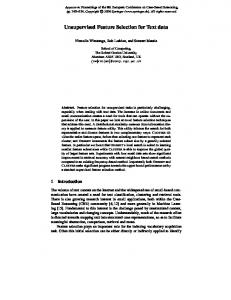
4.2. Results We evaluate the feature selection methods on the three data sets. For each data set, five different feature lists are obtained by using the five filtering methods respectively. When the construction of transition matrix, top 5000 (2500 * 2) of each list are selected as the input list. Once the new feature lists are obtained, top 200, 500, 1000, 1500, 2000, 2500 elements of each list are chosen to represent samples respectively. Each text set is divided into two equal parts: one is for training and the other is for testing. CS1 set Fig.3 shows the performances of the five feature selection methods and the two new methods on the test part of CS1. It can be observed from Fig.3 that the two new methods (FR-MC1 and FR-MC4) achieve similar or better performances than all other methods. Between FR-MC1 and FR-MC4, FR-MC1 achieves the better overall performance. When the number of the features is 500, FR-MC1 yields the highest accuracy (0.9518) while all the values achieved by other methods are below 0.95. MI and BNS behave poorly on this data set. CS2 set Fig.4 shows the performances of the five feature selection methods and the five aggregation methods on the test part of CS2. From Fig.4, the best two methods are IG and FR-MC1. The overall performances of MI and BNS are inferior to others. Although the overall performance of FR-MC4 is worse than CHI and WLLR, the highest accuracy FR-MC4 achieves equals to that of WLLR and higher than that of CHI. ES1 set Fig.5 shows the performances of the five feature selection methods and the two filtering rank
0.88 200
500
1000
1500
IG
MI
CHI
WLLR
FR-MC1
FR-MC4
2000
2500 BNS
Figure 4. Classification results on CS2 set
aggregation methods on the test part of ES.1 From Fig.5, one can observe that FR-MC4 and BNS achieves similar classification results and outperform others. FRMC1 performs inferior to them but also better than the left methods: IG, WLLR, CHI and MI. ES2 set Fig.6 shows the performances of the five feature selection methods and the two filtering rank aggregation methods on the test part of ES2. It can be observed that MI achieves the best results though it is the worst in other three data sets, which indicates that each filtering method has its own merit. FR-MC4 outperforms others except MI and BNS. FR-MC1 obtains similar results with IG. We can get that the performances of both FR-MC1 and FR-MC4 are not below the average.
4.3. Discussion We can compare each classical method with the proposed new methods (FR-MC1 and FR-MC4). For FR-MC1 and IG, FR-MC1 outperforms IG on CS1 and ES1; RF-MCI performs inferior to IG only on CS2 and they achieve similar results on ES2. For FR-MC4 and CHI, we can obtain the same comparing conclusion with that of FR-MC1 and IG. In all, both FR-MC1 and FR-MC4 behave robust on all the data sets. They shows better or comparable performance then the other methods including IG and CHI while in text classification, IG and CHI are reported to be the two most effective methods [16]. Note that we aim to find a feature selection method which can achieve appropriate performance in most cases instead a super method which is able to achieve best results in all cases. We can get that the proposed framework with its two concrete methods provides a
1 0.97
0.95
0.92
0.9 0.85
0.87
0.8 0.75
0.82
0.7
0.77 200
500
1000
1500
2000
IG
MI
CHI
WLLR
FR-MC1
FR-MC4
2500 BNS
Figure 5. Classification results on ES1 set
feasible way with the probability of choosing an inappropriate features is reduced. That is, though the fusion framework can not ensure its results are the best, it is able to ensure that the results are above the average most probably and some times the best. Consequently, the “selection trouble” is alleviated.
5.
Conclusions
In this paper, we propose a fusion framework for text feature selection. Our framework applies traditional filtering feature selection methods to produce several feature rank lists and then utilizes rank aggregation technique to fuse the rank lists. This framework provides a feasible way to combine different feature rank criterions, which is able to alleviate the “selection trouble” when there are so many available filtering methods (criterion). Based on the framework and Markov chains method, two new feature selection algorithms are introduced: FR-MC1 and FR-MC4. To alleviate the drawbacks of Markov chains methods, we study the properties of the state transition matrix and propose a perturbation algorithm. Four experiments are conducted on four public text data sets. The results suggested that the proposed new feature selection algorithms are able to yields promising performance and comparable to other classical filtering methods. Evaluating a single feature is also essential in hybrid feature selection methods. It is possible that our study can improve the studies of hybrid feature selection.
6. Acknowledgement This work is partly supported by NSFC (Grant No.60672040 and 60672040) and the National 863
200
500
1000
1500
2000
IG
MI
CHI
WLLR
FR-MC1
FR-MC4
2500 BNS
Figure 6. Classification results on ES2 set
High-Tech R&D Program of China (Grant No. 2006AA01Z453).
7. References [1] I. Guyon et al., “An Introduction to Variable and Feature Selection”, Journal of Machine Learning Research, 3 (2003) pp.1157-1182. [2] Z. Zhu et al., “Wrapper-filter feature selection algorithm using a memetic framework”, IEEE Trans. System Man and Cybernetics. Part B, 2007, Vol.37, No.1, pp.70-76. [3] L. Molina et al., “Feature Selection Algorithms: A Survey and Experimental Evaluation”, Pro. of International Conference on Data Mining , 2002, pp.306-313. [4] X. Geng et al., “Feature Selection for Ranking”, Pro. of ACM SIGIR Conference, 2007, pp.407-414. [5] A. Dasgupta et al., “Feature Selection Methods for Text Classification”, Pro. of ACM KDD Conference, 2007, pp.230-239. [6] L. Breiman et al., “Classification and regression trees”, Wadsworth and Brooks,1984. [7] E. Cant´u-Paz et al., “Feature Selection in Scientific Applications”, Pro. of ACM KDD Conference, pp.788793, 2004. [8] C. Dwork, “Rank aggregation revisited”, Manuscript, http://www.eecs.harvard.edu/~michaelm/CS222/rank2.p df , 2001. [9] C. Dwork et al., “Rank aggregation methods for the Web”, Pro. of World Wide Web Conference , 2001, pp. 613622. [10]M. Farah et al., “An Outranking Approach for Rank Aggregation in Information Retrieval”, Pro. of ACM SIGIR Conference, 2007, pp.591-598. [11] M. Renda et al. “Web Metasearch: Rank vs. score based rank aggregation methods”, Pro. Of ACM SOAC Conference, 2003, pp.841-846. [12]J. Lee et al., “Analyses of multiple evidence combination”, Pro. of ACM SIGIR Conference, 1997, pp. 267-276.
[13] H. Young et al., “A consistent extension of Condorcet's election principle”, SIAM Journal on Applied Math, 1978, 35(2):285-300. [14] G. Forman, “An extensive empirical study of feature selection metrics for text classification”, Journal of Machine Learning Research, 2003,3(1):1533-7928. [15]T.Liu et al, “An evaluation on feature selection for text clustering”, Proc. of International Conference on Machine Learning, 2003, pp.488-495. [16]Y.Yang et al., “A Comparative Study on Feature Selection in Text Categorization”, Proc. of International Conference on Machine Learning,, 1997 pp.412-420. [17]V. Ng et al., “Examining the Role of Linguistic Knowledge Sources in the Automatic Identification and Classification of Review”, Proc. of the COLING/ACL Main Conference Poster Sessions, 2006, pp.611–618. [18]K.Nigam et al., “Text classification from labeled and unlabeled documents using EM”, Machine Learning, 2000, 39(2):103-134. [19]S. Householder, “The Theory of Matrices in Numerical Analysis”, Blaisdell Publishing Company, 1964. [20]T. Joachims, “Text Categorization with Support Vector Machines: Learning with Many Relevant Features”, Proc. the 10th ECML, pp.137-142, 1998. [21]http://www.sogou.com/labs/dl/t.html. [22]S. Tan et al., “A Novel Refinement Approach for Text Categorization”, Pro. of ACM CIKM Conference, pp.469-476, 2005. [23]http://www.nlp.org.cn/docs/download.php?doc_id=294 [24] http://sewm.pku.edu.cn/QA/ [25]http://www.csie.ntu.edu.tw/~cjlin/papers/guide/guide.pdf [26]http://kdd.ics.uci.edu/databases/reuters21578/reuters215 78.html
Appendix: Let C denote the set of absorbing states and C be the set of non-absorbing states. If using the original state transition matrix constructed by MC4, any state in C will rank better than all states in C . This correctly reflects the state orderings. We concern about whether this relationship can hold after perturbation. Without loss of generality, we can exchange the labels of states such that the states in C can be arranged to the front of the list. Then the state transition matrix constructed by MC4 can be written as:
⎡ P|C' |×|C | P=⎢ ⎢ P '' ⎣ |C |×|C |
⎤ ⎥ ''' P|C |×|C | ⎥⎦ 0
(A-1)
We have the following lemma: Lemma A.1: Let (A-1) be the state transition matrix obtained by MC4. If M is modified to P by Eq. (14),
states in C are still ordered better or at least no worse than all states in C by P. Proof: Let l be an arbitrary state in C and k be an arbitrary element C , v be the left principal eigenvector. The corresponding values of l and k in v are vl and vk respectively. Note that the left principal value of the state transition matrix equals to 1. We denote P as [ P1 , , Pl , ] . We have:
v ⋅ Pl = vl and v ⋅ Pk = vk or
∑
pil vi +
∑
pik vi +
i∈c ,i ≠ l
i∈c ,i ≠ l
∑
j∈c , j ≠ k
∑
p jl v j + pll vl + pkl vk = vl (A-2)
j∈c , j ≠ k
p jk v j + pkk vk + plk vl = vk (A-3)
According to MC4 and Eq. (14), we can obtain:
pil = mil + ε / N
p jl = (1 + ε ) / N pll = mll − ε ( N − 1) / N
pik = ε / N
(A-4)
p jk = m jk + ε / N pkk = mkk − ε ( N − 1) / N Plugging Eq. (A-4) into (A-2) and (A-3) and Using Eq. (A-2) subtracts (A-3), we have:
vl − vk = (1 + ε − mkk ) −1 ( ∑ mil vi + i∈c , i ≠ l
∑
(1 / N − m jk )v j +( mll − mkk )vl + vk / N )
j∈c , j ≠ k
(A-5) Note that we have the following constraints:
ε >0
m jk ≤ 1 / N mll >= 1− | C | / N
(A-6)
mkk