Rapidly Finding CAD Features Using Database Optimisation - CiteSeerX

Rapidly Finding CAD Features Using Database Optimisation Zhibin Niua,∗, Ralph R. Martina , Frank C. Langbeina , Malcolm A. Sabinb a

School of Computer Science & Informatics, Cardiff University, UK b Numerical Geometry Ltd., Cambridge, UK

Abstract Automatic feature recognition aids downstream processes such as engineering analysis and manufacture. Not all features can be defined in advance; a declarative approach allows engineers to specify new features without having to design algorithms to find them. Naive translation of declarations leads to executable algorithms with high time complexity. Database queries are also expressed declaratively; there is a large literature on optimising query plans for efficient execution of database queries. Our earlier work investigated applying such technology to feature recognition, using a testbed interfacing a database system (SQLite) to a CAD modeler (CADfix). Feature declarations were translated into SQL queries which are then executed. The current paper extends this approach, using the PostgreSQL database, and provides several new insights: (i) query optimisation works quite differently in these two databases (ii) with care, an approach to query translation can be devised that works well for both databases, and (iii) when finding various simple common features, linear time performance can be achieved with respect to model size, with acceptable times for real industrial models. Further results also show how lazy evaluation can be used to reduce the work performed by the CAD modeler, and how estimating the time taken to compute various geometric operations can further improve the query plan. Experimental results are presented to validate our main conclusions. Keywords: Feature recognition, Database query planning ∗

Corresponding author Email addresses: [email protected] (Zhibin Niu), [email protected] (Ralph R. Martin), [email protected] (Frank C. Langbein), [email protected] (Malcolm A. Sabin) Preprint submitted to Computer-Aided Design

March 24, 2015

1. Introduction Feature recognition aims to extract certain substructures from a solid model; it has been the subject of extensive research during the past thirty years [1, 2, 3]. One major application of feature recognition is for computer aided process planning, the generation of sequences of instructions for manufacturing [4]. More recently, its use for simplifying engineering analysis has become more important: small features may be removed or replaced by stress concentration factors, for example. Furthermore, meshing of defeatured models is typically both quicker and more robust, and as the resulting mesh has fewer elements, the time needed for analysis is reduced [5, 6, 7]. Manually finding feature instances is tedious, and in extreme cases, infeasible to carry out reliably, as complex models may have tens of thousands of small features of many types and forms. Fig. 1, which extends a figure in [8], gives some typical industrial features. Some are common, such as slots and holes, while others such as notches may be infrequent. Traditional feature recognition algorithms face two challenges. Firstly, different applications need to find different features: parts of a shape which are important for machining may be quite different to those which can be ignored during engineering analysis. In fact, system builders cannot anticipate in advance all applications to which feature finding may be put, and all things a user may consider to be a feature. Ultimately, therefore, users of a feature finder must themselves be able to define features. The second issue is that many approaches to feature finding have high computational complexity: times taken to find features can rise rapidly when dealing with complex features and large detailed models. The first issue above is challenging as it is difficult for engineering end users to define their own effective algorithms for finding features. One solution is to use a declarative approach: this allows users of a feature finder to simply state what properties a feature has, and how a feature is composed, rather than having to give an algorithm to find instances of the feature. However, naively turning such a definition into an algorithm results in a series of nested loops, which takes far too long to execute for any non-trivial feature. Gibson pioneered such declarative approach, and considered six specific optimizations which could be used to transform the naive code into a faster algorithm [9, 10]. He showed that this could effectively solve various 2D fea2

(a) Through-hole

(b) Cone

(c) Buttress

(d) Fin

(e) Pocket

(f) Pyramid

(g) T-junction

(h) X-junction

(i) I-beam

(j) C-beam

(k) Rib

(l) Notch

Figure 1: Common industrial features, including some noted in [8]

3

ture recognition problems. However 3D problems involving complex features and large models required further optimisation. In previous work [11], we made the significant observation that relational database management systems (DBMS) also use a declarative language, SQL, to formulate database queries, and that much research has gone into optimising the executable plans into which the queries are translated [12]. We demonstrated that these optimisations built into a DBMS could be taken advantage of when turning declarative feature definitions into executable algorithms for finding features. We used a high-level declarative feature language, allowing end-user engineers to define new features of interest. Finding fetures—instances of these declarations—was translated into an SQL query, which was then input to a relational DBMS (SQLite) coupled to a CAD modeler (CADfix) as a back end. Geometric and topological information is processed instead of data from tables. Our main conclusions were as follows: naive translation of a feature declaration based on e distinct entities (faces, edges, vertices, subfeatures, etc.) leads to an execution plan with e nested loops, so feature finding takes time O(ne ) for a model with n entities. However, SQLite’s optimiser was often capable of optimising such plans into ones taking time O(n2 ) for simple features, giving a significant improvement, and times which are viable for a real system. We discussed which optimizations in SQLite’s query optimizer led to this performance, and also compared them to the specifically crafted optimizations devised by Gibson [10]. This paper builds upon that previous work. We have replaced the SQLite database engine with PostgreSQL, as its query optimizer is considered to be more powerful (it also allows more complex SQL queries which we expect to be useful in future research). Doing so has provided us with several further insights: (i) query optimisation works quite differently in these two databases, (ii) with care, an approach to query translation can be devised that works well for both databases, despite these differences, (iii) for various simple common features, more or less linear performance can be achieved with respect to model size, and (iv) acceptable performance can be achieved for real industrial models. PostgreSQL is clearly a more suitable database engine for a CAD feature recogniser, as SQLite typically gives quadratic performance. We also present further results. We have investigated (i) how lazy evaluation can be used to reduce the work performed by the CAD modeler, and (ii) how estimates of the time taken to compute various geometric operations can be used to further improve the query plan. We also analyze how linear time performance is achieved, and compare the PostgreSQL optimisation approach 4

with SQLite query optimization and Gibson’s work. Experimental results are presented to validate our main conclusions. The rest of this paper is organized as follows. Section 2 discusses previous work. Section 3 overviews our architecture, while Section 4 details our contributions to feature recognizer speed: effective translation, lazy evaluation, and selectivity. Section 5 presents our experimental results and discusses them, while Section 6 concludes the paper and considers future work. 2. Previous Work 2.1. Feature recognition We start by briefly summarising prior work on feature recognition, much of which is historical—yet the need for feature recognition is perhaps greater now than ever before. Since the seminal work on geometric model analysis and classification by Kyprianou [13], much work has considered feature recognition. Various different approaches have been taken [4], and various ways can be used to classify them: according to how features are defined, according to the approach used to finding them, according to the application area, whether the method is fully automatic or interactive, and so on. One approach is design-by-features, but this is generally unsatisfactory as it only considers features for one purpose, typically manufacturing, and a completely different set of features may be relevant in, say, engineering analysis. It also cannot handle legacy models not designed in this way. The alternatives are automatic feature recognition and interactive feature recognition. The former has attracted the most attention, with a certain degree of success [3, 4]. Many approaches are rule-based [4], but lack of suitable domain knowledge acquisition mechanisms has been a limiting factor. Most contemporary systems deal mainly with fixed, orthogonal features, and less attention has been paid to non-orthogonal and arbitrary features [4]. Interactive feature recognition is more flexible, either allowing manual assistance when finding features, or allowing the user to define new features. For example, Gao [6] allows features to be defined graphically interactively, and a graph-based feature recognition method is used to segment a CAD mesh model to a region-level representation from which features are extracted. Feature recognition systems can be classified according to the underlying CAD model representation, typically boundary representation (B-rep) or constructive solid geometry (CSG). Features are defined in terms of relations 5

between components which form substructures. Algorithms can also be categorised according to approach [3, 4], three main ones being graph-based, volumetric decomposition, and hint-based. The graph-based approach first translates a B-rep model and a target feature into attributed face adjacency graphs (AAG), and then performs graph matching. There are many variants of this basic approach; a few allow users to define their own features, and work well for simple features [14, 15]. There are two main drawbacks to graphbased approaches. Firstly, they are less successful at coping with interacting features, and features with variable topology, like n-sided prisms for any n. Secondly, they are slow. In general, subgraph matching has exponential complexity. Thus, some partitioning strategy or hints must be used [16, 17], but even then times can be too long for large models or complex features. Volume decomposition and recomposition approaches are also quite general, and good at dealing with interacting features, but they are again computationally intensive and limited to low degree analytical surfaces [16]. Hint-based approaches are computationally efficient for small features but use hard-coded features—it is not easy for end users to modify them or define new ones [16]. Most work concerns fixed algorithms for finding predetermined features, and is not flexible enough to let engineers define their own features, a necessity for many particular real-world applications. Features may however be represented by data instead of code. In the former case, execution algorithms may be generated automatically. For example, in [18] features are defined in a special language embedded in Common Lisp, using a surfacebased attributed adjacency graph which satisfies additional conditions such as topological restrictions. A serious problem facing approaches based on code generation is the computational complexity of feature finding: a naive execution plan involves multiple nested for loops, one for each entity involved in the feature. Gibson [10] showed how to overcome this problem to some degree, giving six specific ways to optimize execution plans; we build upon his ideas. Feature recognition methods can be specialised to focus on a specific application domain such as machining [19], injection moulding [8], NC milling of free-form surfaces [20, 21], blends [22], and assembly [23]. Taking one specific domain, in recent years, computer aided engineering analysis has become ever more widely used, leading to a requirement for model simplification, the aim being to remove (typically small) features which have little effect on the analysis results. The resulting models can be meshed more quickly and robustly for finite element analysis, and in turn analysed more quickly, as the 6

meshes are simpler. Feature identification for simplification has traditionally been done by hand. Models may contain tens of thousands to millions of edges and faces, amongst which there may be many small features. Manually finding features is tedious and error prone, leading to interest in methods to find analysis features [5]. Different applications need different kinds of features, so typically, such specialised recognition methods are not flexible enough as a basis for a universal feature recognition system, in which the user can define arbitrary new features. Instead, engineers have to choose an appropriate approach based on priorities such as design objectives in a given application field [16]. A key point often overlooked is that it is infeasible to hard-code all possible useful features for all possible domains in advance [16]—application domain engineers need to be able to supply their own feature definitions for new tasks. However, engineers who understand what a feature is may not be expert in devising geometric algorithms to find such features. Useful methods must also take into account the large number of edges and faces in real models: efficient methods are needed, and simple algorithms devised by an engineer are unlikely to be efficient. He may not be an expert programmer, even if he is an application domain expert. In summary, an ideal feature recognition system should be general, allowing end users to define new kinds of features relevant to their application, but it should leave the system to devise an efficient algorithm. This suggests a declarative rather than procedural approach to feature definition. However, the algorithm generator will need optimisation techniques to ensure sufficient performance. 2.2. Database query optimisation Information is retrieved from relation databases using declarative queries, and if they are naively translated into execution plans, the time taken is far too long. There is thus a large body of work on optimising query processing. This can be put to use to efficiently retrieve features from CAD models using declarative feature definitions. We start by very briefly reviewing the structure of a database query in SQL, the high level declarative language typically used [24]. An example might be: 1 2 3

SELECT c . tstamp FROM commits c , actions a WHERE a . file IN

7

4 5 6 7 8

( SELECT id FROM files WHERE path = ... ) AND a . commit_id = c . id AND c . id >5 GROUP BY c . tstamp DESC HAVING agg () ; Listing 1: Example SQL query

This is an implicit join SQL query. Items after SELECT name the information the user wishes to retrieve from the database. The keyword FROM is followed by several range tables, which are the source of the target information. WHERE specifies various predicates the selected elements should satisfy. They can include subqueries such as the SELECT clause in brackets; they can also be join predicates like the one equating a.commit_id to c.id, which connects two range tables via a common value. The predicates in WHERE statements are evaluated on all tuples, generating a temporary target list, while the HAVING clause further aggregates the temporary target list to produce the final results. We will use this idea later. When the query is executed, a query optimizer is used to determine a suitable plan, or algorithm, from the declarative form of the query. Considerable effort may be put into query planning, as the savings over straightforward plans may be significant, and indeed turn an infeasible query into a feasible one. Query optimisation is a mature field [25]. Normally, a declarative query is first turned into a relational calculus expression, and the query optimizer then generates various execution paths with equivalent results, using two stages: rewriting and planning [25]. The former rewrites the declarative query in the expectation that the new form may be more efficient. An example of this approach is sargable rewriting (i.e. a transformation to take advantage of an index). Planning transforms the query at a procedural level, via relational algebra transformations. Then a cost based planner is used to choose the plan predicted to be fastest based on statistical information about the database. System-R, one of the earliest databases to support SQL, pioneered such optimzation [26]. Its use of dynamic programming to select the best query plan has been adopted by most commercial databases [25]. Space precludes a full discussion of query optimisation technology; for more information see [12]. However, we note that the planner may generate the search space by transforming the query in the following ways: Generalizing join sequencing Join clauses combine records from two or more tables in a database. There are many kinds of joins, such as explicit joins, implicit inner joins, left joins, full outer joins, cross joins, 8

etc. This step finds an efficienty execution order for procssing multiple joins. Because join tuples are not necessarily symmetric, and the operations are commutative and associative, a translated execution tree with Cartesian products may result in poor performance for some orders of evaluation [26]. Approaches include turning asymmetric one-sided outer joins into equivalent but re-orderable expressions [27] by shuffling GROUP BY and JOIN [28], an important optimization supported by most current database systems [29, 30, 31, 32] Multi-block query transformation A multi-block query including several select-from-where structures in a single query can be converted to a single block query via view merging, nested subquery merging (also called subquery flattening [29]), and semijoin-ike techniques [26]. Scan methods Database systems use various methods, including sequential scans, index scans, and bitmap index scans, to scan tables. Index and bitmap index scanning are much more efficient than sequential scanning, because only parts of the table have to be considered [30]. The planner chooses an appropriate scan method based on selectivity, a quantity which determines the effectiveness of an index in terms of the proportion of the data filtered out [33]. Join optimization Declarative joins can be translated into procedural algorithms in various ways. The main approaches include use of nested loops, hash joins, and merge joins. Nested loops are normally used for small tables while the other approaches work much better for large tables [33]. Such optimizations is also widely used in mainstream database systems [30, 31, 32] 2.3. Gibson’s work As our work follows on from Gibson’s, we now describe his contribution in more detail. He suggested that a declarative approach to feature definition could be an effective solution to the problem of allowing user-defined features [9, 10, 34]. He also noted that naive translation of the declarative form into an execution plan leads to very inefficient algorithms, and that optimisation of such plans is necessary. He defined features in a language with similarities to EXPRESS [35]. Features are based on entities, and predicates linking them. Such a declaration can be rewritten as a set of nested FOR loops, one per entity in the definition, 9

and IF statements, one per predicate. Executing this takes exponential time in the number of entities in the feature definition, so is infeasible for anything but trivial features. Gibson investigated six strategies for optimizing this basic plan; they are clearly related to those used in database optimization, although Gibson did not consider this point of view. His strategies belong to four categories with respect to their effect on time complexity: Strength reduction and loop re-sequencing Both methods aim to reduce time spent inside a nested loop. They reduce recognition time by some constant factor but do not change the time complexity, which remains O(nk ) where k is number of loops and n is the total number of entities in the model. In SQL, join reordering is analogous to loop re-sequencing [36]. Entity classification and featuretting These are both ways of splitting a declarative definition into parts. This reduces the time complexity from O(nk ) to O(max(nk11 , . . . , nkmm )) where m is the number of parts and ni is the number of entities in part i. Database systems do not typically automatically split queries into parts, so we cannot rely on the optimser in a database engine to do this for us. However, if the user defines features in terms of subfeatures (a natural divide-and-conquer approach to problem solving), such a split is achieved manually, reducing time complexity. Indexing Precomputing an index allows required entities to be immediately determined, rather than having to check each one by one during query processing, and is an effective technique used both in Gibson’s approach and database engines. Time improvements depend on the selectivity of the index. Assignment This approach narrows the search space by finding WHERE statements containing equalities and associated conditions. The key idea is to replace an inner loop by the results satisfying the outer loop conditions, reducing the time complexity. Database subqueries share a common goal with Gibson’s assignment approach, but adopt flattening which works differently in detail. 2.4. Our previous work Our previous work [11] extended Gibson’s work from 2D to 3D models, more typical of real engineering, and considers a greater number of basic 10

entities. We followed his declarative approach, but rather than devising an ad-hoc set of query optimisations, we took advantage of database optimisation techniques. We translated declarative feature definitions into SQL queries which could then be automatically optimised by a database engine, SQLite, before evaluation using a CAD modeler, CADfix. SQLite has a compact but effective query optimizer [29]: it provides sargable rewriting including BETWEEN and OR optimizations, and provides algebraic space and method-structure space transformations such as reordering joins, subquery flattening, automatic indexing and group-by optimizations. Its nearest neighbor heuristic planner provides an efficient polynomial-time algorithm to select a good plan. Our experiments showed that this approach could effectively find various basic features (in particular through-holes, notches, and slots) in models, and experimentally showed that the time complexity is reduced from exponential to approximately quadratic for these simple features. The main optimization processes used by SQLite to achieve this are reordering joins, using a covering index, and subquery flattening. In this paper, we have replaced the database engine by PostgreSQL. One goal was to see whether the optimizations provided by SQLite could be replicated, and to determine whether different database engines would arrive at similar query execution plans when used for feature recognition. As our results later show, SQLite and PostgreSQL take very different approaches to query optimization. Our previous approach for translating feature declarations into SQL queries which worked well for SQLite was much less successful when used with PostgreSQL. This led us to reconsidering how to perform translation, leading to a new approach which works well with both databases. We also show that PostgreSQL query optimization is more powerful for reasons explained later; the result is now that simple features can be found in linear time. Further motivation for moving to PostgreSQL was its more powerful indexing facilities, and facilities for recursive SQL queries which we hope to make use of in our future work. We also extend our earlier work by considering further improvements that can be brought about by lazy evaluation, and by using estimates of time required to compute various geometric operations. 3. Optimization in a feature recognizer While a declarative approach enables users to write feature definitions rather than algorithms for finding them, but naively turning them into algo11

rithms leads to a series of nested loops with exponential time complexity with respect to the number of entities in the feature definition. Optimizing such algorithms is therefore essential for a declarative approach to be of realistic industrial use. As we have already explained, our goal is to let a database engine carry out this optimization for us, allowing us to leverage the large body of research on database query optimization. The first important contribution of this paper is an approach to translating feature definitions into carefully designed queries, which work well for multiple database systems. Different database systems take different approaches to query optimization, and if the query is presented to a database is in a form which is not well handled by the optimizer in a particular database, poor performance will be the result. The second idea we consider is lazy evaluation. Some geometric predicates, e.g. determining whether the area of a curved face exceeds a threshold, require intensive calculation. For efficiency, rather than evaluating such a predicate for all relevant entities, it is better to only evaluate it for those entities for which it is definitely needed. For example, if a face fails to meet some other constraint such as being connected to a certain edge, we may never need its area. Thirdly, when we do have to perform geometric computations, some are much cheaper than others. It may be quicker to perform a simple computation on many entities rather than a very slow computation on just a few entities. In cases when multiple predicates filter a list of entities, determining how many entities there are of various kinds, and how long different predicates are expected to take to compute, can be used to choose the best order for applying each filter. The second and third optimizations above are typically absent from database systems, as most queries are based on reading data from tables, which is quick, and takes a more or less constant amount of time. We now briefly summarise our system architecture, which remains essentially unchanged from our earlier work, apart from the additional selectivity module and training models; see [11]. The feature recognizer includes a translator, importer, query planner, executor, and selectivity trainer, interfaced to a CAD modeler. Commands to open a model, or draw feature instances on the CAD model, are handled by the command analyzer, and requests are passed to the modeler. Another command is used to declaratively define a feature. When some further command requires execution of the definition, the translator turns it into SQL which is in turn optimized by the query plan12

Figure 2: Feature recognition architecture

ner internal to the chosen database engine. The importer analyzes the query and caches necessary simple relations retrieved from the CAD modeler for speed; only topological relations and edge convexity information are treated in this way. The query planner analyzes the query as well as the numbers of entities in the basic topological relations to determine the expected cheapest plan. This takes into account the cost of computing each predicate. The executor executes the chosen query plan, using data from the local cache and other information requested directly from the CAD modeler. The resulting feature instances can be output in text format or drawn on the original CAD model. In this implementation of our approach, PostgreSQL is used as the DBMS engine—it is free, has open source which aids understanding of its query optimizer, and has clearly structured code which facilitates linking it to the CAD modeler. PostgreSQL supports a range of query optimization approaches. 13

The most important include (i) alternative ways to access data using sequential scans, bitmap index scans, or index scans according to filter selectivity (using statistics obtained by ANALYZE), (ii) alternative ways of processing joins to shrink the search space and reduce time complexity, using nested loops, hash joins, merge joins or procedural code, and (iii) reordering join sequences. PostgreSQL’s optimizer uses System R’s dynamic programming approach when the number of tables is small, but switches to a genetic algorithm to solve the join ordering problem when there is a large number of FROM tables [37, 38]. CADfix [39, 40] is used as the CAD modeler. It is a commercial geometry translation and repair package primarily intended for 3D model data exchange between different engineering systems and applications. It already provides some defeaturing tools, although we do not make use of these. We use CADfix (via its API) to load CAD models (and repair them to ensure consistent, connected topology), and to interrogate their topology and geometry. It is also used to draw the features found. 4. Improvements to Query Translation and Execution We now discuss the three main contributions of this paper which improve query translation and execution: effective translation, lazy evaluation and predicate ordering. 4.1. Effective translation The first contribution considers how to translate declarative feature definitions into SQL queries which can be efficiently processed by the database engine, independently of how it subsequently performs query optimization. 4.1.1. Approach Features are defined in terms of necessary component entities, relationships between them, and characteristics they should exhibit. The entities include faces, edges and vertices, as well as subfeatures. Predicates provided include: 1 2 3 4 5 6

Bounds ( edge_id :e , face_id : f ) V_bounds_e ( vertex_id :v , edge_id : e ) Valency ( face_id :f , int : i ) F a c e _ h a s _ n u m b e r _ o f _ v e r t i c e s ( face_id :f , int : imin , int : imax ) F a c e _ h a s _ n u m b e r _ o f _ e d g e s ( face_id :f , int : imin , int : imax ) F a c e _ h a s _ n u m b e r _ o f _ l o o p s ( face_id :f , int : imin , int : imax )

14

7 8 9 10 11

12 13 14 15 16 17 18 19 20 21 22 23 24 25 26 27 28 29 30 31

Fac e_has_ geomet ry ( face_id : f1 , facetype : t ) P l a n e _ n o r m a l _ a l i g n e d _ w i t h i n ( face_id :f , vector :v , angle : a ) C y l i n d e r _ a x i s _ a l i g n e d _ w i t h i n ( face_id :f , vector :v , angle : a ) C o n e _ a x i s _ a l i g n e d _ w i t h i n ( face_id :f , vector :v , angle : a ) E l l i p s o i d _ a x i s _ a l i g n e d _ w i t h i n ( face_id : f1 , vector : v1 , angle : a1 , vector : v2 , angle : a2 ) T o r u s _ a x i s _ a l i g n e d _ w i t h i n ( face_id :f , vector :v , angle : a ) C o ne _ a ng l e _i n _ ra n g e ( face_id :f , angle : amin , angle : amax ) S phe re _c en tr e_ ne ar ( face_id :f , point :p , real : r ) E l l i p s o i d _ c e n t r e _ n e a r ( face_id :f , point :p , real : r ) Tor us_cen tre_ne ar ( face_id :f , point :p , real : r ) S p h e r e _ r a d i u s _ i n _ r a n g e ( face_id :f , real : rmin , real : rmax ) C y l i n d e r _ r a d i u s _ i n _ r a n g e ( face_id :f , real : rmin , real : rmax ) C o n e _ m i n _ r a d i u s _ i n _ r a n g e ( face_id :f , real : rmin , real : rmax ) C o n e _ m a x _ r a d i u s _ i n _ r a n g e ( face_id :f , real : rmin , real : rmax ) T o r u s _ r a d i i _ i n _ r a n g e ( face_id :f , real : rmin1 , real : rmax1 , real : rmin2 , real : rmax2 ) E l l i p s o i d _ r a d i i _ i n _ r a n g e ( face_id :f , real : rmin1 , real : rmax1 , real : rmin2 , real : rmax2 , real : rmin3 , real : rmax3 ) F ace _a re a_ in _r an ge ( face_id :f , real : rmin , real : rmax ) Edg e_has_ geomet ry ( edge_id : e1 , edgetype : type ) Convexity_is ( edge_id : e1 , convexitytype : type ) E d g e _ l e n g t h _ i n _ r a n g e ( edge_id :e , real : rmin , real : rmax ) B o d y _ h a s _ n u m b e r _ o f _ f a c e s ( body_id :b , int : imin , int : imax ) B o d y _ h a s _ n u m b e r _ o f _ e d g e s ( body_id :b , int : imin , int : imax ) B o d y _ h a s _ n u m b e r _ o f _ v e r t i c e s ( body_id :b , int : imin , int : imax ) Listing 2: Supported predicates

The predicates—truth functions returning a Boolean answer—are carefully chosen to be simple. This both aids the user who is writing feature definitions, and in translating the definitions into queries. For example, when using Bounds(edge_id:e,face_id:f), the user does not need to think in terms of following all edges around the boundary of a face, but simply in terms of which edges belong to that boundary. The translator transforms each predicate into a query fragment; multiple predicates are connected using AND. As noted, there are various ways to translate SQL queries and alternative plans differ in efficiency. Predicate clauses can include attribute predicates and relational predicates. The former typically involve only a single entity and some condition that the entity must satisfy, encoding a binary relation. Such predicates can be written as SQL fragments in a straightforward way. For example: 1

Definition :

Convexity_is ( edge , convex )

15

2

SQL fragment :

edge . convexity = convex

These predicates act as filters. A query optimizer can efficiently deal with them by indexing the data. Relational predicates are more complex and typically involve two (or more) entities, indicating some relationship between them. Bounds(edge, face) is of this type; it indicates connectivity of some face and some edge. It is one of the most important predicates, used in almost every feature definition. Since the edge and face are arbitrary, when executing a feature query, we must in principle iterate over all faces and all edges to determine which ones satisfy this relationship. As such a predicate involves two variables, it cannot be effectively written as a filter (in our previous paper, Bounds(edge, face) was translated as an EXISTS subquery, but further experiments have show this not to be efficient). Our previous work [11], based on the SQLite database, straightforwardly translated feature definitions into SQL queries using a series of EXISTS clauses. Entities satisfying bounds predicates linking edges and faces (and similar predicates) were found using a preloaded, cached range table: 1 2

Definition : SQL fragment :

3 4 5

Range table :

bounds ( e1 , f1 ) ; EXISTS ( SELECT bounds . edge FROM bounds WHERE bounds . face = f1 . face AND bounds . edge = e1 . edge ) bounds ( edge int , face int ) ;

As SQLite effectively performs self-join optimization, bounds were handled efficiently, allowing simple features could be found in time roughly O(n2 ) for models with n entities. However, on replacing SQLite with PostgreSQL, we found that this was no longer the case. PostgreSQL has no self-join optimisation, and instead uses a strategy based on cross-joins via a Cartesian product. Such optimisation fails to reduce complexity of nested loops corresponding to multiple predicates, and even for simple models, it would take days to return results. This led us to rethink the way translation was performed. For flexibility, the translator should work in a way which leads to good query processing times independently of the choice of the underlying database engine used.

16

Assuming that we are dealing with manifold models1 , each edge bounds only two faces, so the number of bounds relationships is twice the number of edges. We can take advantage of this observation by, instead of thinking in terms of edge-face pairs joined by a bounds relationship, thinking in terms of edge-face1-face2 triples. We extract and cache these in a full-edge-form table. For a given edge, the triples edge-face1-face2 and edge-face2-face1 are both cached, as a feature definition might insist that face1 has a lower id than face2, or vice versa (to prevent a symmetric feature from being reported multiple times with different labelings, for example). This doubles the table size, but provides more flexibility, and has little impact on performance, as we show later. Feature declarations can be automatically rewritten to use the full-edgeform relationship, rather than the bounds relationship. Feature definitions often specify e.g. that two edges border the same face, or that they belong to different faces. This can be expressed using an equality or inequality predicate. The translator can simply and efficiently turn the bounds relations in the user’s definition into full-edge-form predicates automatically. For example, the SQL fragment full_edge_e1.f2=full_edge_e2.f1 corresponds to the need to find a pair of tuples with patterns ei, fa, fb and ej, fb, fc in the full-edge-form table. Typically, many relations of this kind will occur in the WHERE clause of the generated query. This approach replaces the need to iterate over all possibilities to find a pair of a face and an edge satisfying a bounding relationship by simply having to determine those few tuples which match a pattern indicating equality. Most database systems can recognize such relations as corresponding to inner joins, and can readily optimize them [30, 31, 32]. An example of a definition of a notch feature from our previous work is given in Fig. 3. (It includes explicit statements of inequality of various faces, an issue we return to shortly). Our previous approach translation approach for the SQLite database results in the SQL query: 1 2 3 4 5

SELECT f1 . face , f2 . face , f3 . face , f4 . face , e1 . edge , e2 . edge , e3 . edge , e4 . edge , e5 . edge FROM faces AS f1 , faces AS f2 , faces AS f3 , faces AS f4 , edges AS e1 , edges AS e2 , edges AS e3 , edges AS e4 , edges AS e5

1

Even if the models are non-manifold, the number of non-manifold edges is typically small, as is the number of faces around each one, so this idea still works.

17

DEFINE NOTCH AS F1,F2,F3,F4:face; E1,E2,E3,E4,E5:edge; SATISFYING Bounds(E1,F1); Bounds(E1,F2); Bounds(E2,F2); Bounds(E2,F3); Bounds(E3,F1); Bounds(E3,F4); Bounds(E4,F1); Bounds(E4,F3); Bounds(E5,F1); Bounds(E5,F4); Lower_id(F1,F2); Lower_id(F3,F4); Different_id(E2,E1); Different_id(E3,E1); Different_id(E4,E1); Different_id(E5,E1); Convexity_is(E1,CONCAVE); Convexity_is(E2,CONVEX); Convexity_is(E3,CONVEX); Convexity_is(E4,CONVEX); END

Figure 3: Notch feature and definition

6 7 8 9 10 11 12 13 14 15 16 17 18 19 20 21 22 23 24 25 26 27 28 29 30 31 32 33 34 35 36 37

WHERE f1 . face < f2 . face AND f3 . face < f4 . face AND e2 . edge < > e1 . edge AND e3 . edge < > e1 . edge AND e4 . edge < > e1 . edge AND e5 . edge < > e1 . edge AND EXISTS ( SELECT bounds . edge FROM bounds WHERE bounds . face = f1 . face AND bounds . edge = e1 . edge ) AND EXISTS ( SELECT bounds . edge FROM bounds WHERE bounds . face = f2 . face AND bounds . edge = e1 . edge ) AND EXISTS ( SELECT convexity . edge FROM convexity WHERE convexity . type =1 AND convexity . edge = e1 . edge ) AND EXISTS ( SELECT bounds . edge FROM bounds WHERE bounds . face = f2 . face AND bounds . edge = e2 . edge ) AND EXISTS ( SELECT bounds . edge FROM bounds WHERE bounds . face = f3 . face AND bounds . edge = e2 . edge ) AND EXISTS

18

38 39 40 41 42 43 44 45 46 47 48 49 50 51 52 53 54 55 56 57 58 59 60 61 62 63 64 65 66 67 68 69 70 71 72 73 74 75 76 77 78 79 80 81 82

( SELECT convexity . edge FROM convexity WHERE convexity . type =2 AND convexity . edge = e2 . edge ) AND EXISTS ( SELECT bounds . edge FROM bounds WHERE bounds . face = f1 . face AND bounds . edge = e3 . edge ) AND EXISTS ( SELECT bounds . edge FROM bounds WHERE bounds . face = f4 . face AND bounds . edge = e3 . edge ) AND EXISTS ( SELECT convexity . edge FROM convexity WHERE convexity . type =2 AND convexity . edge = e3 . edge ) AND EXISTS ( SELECT bounds . edge FROM bounds WHERE bounds . face = f1 . face AND bounds . edge = e4 . edge ) AND EXISTS ( SELECT bounds . edge FROM bounds WHERE bounds . face = f3 . face AND bounds . edge = e4 . edge ) AND EXISTS ( SELECT convexity . edge FROM convexity WHERE convexity . type =2 AND convexity . edge = e4 . edge ) AND EXISTS ( SELECT convexity . edge FROM convexity WHERE convexity . type =2 AND convexity . edge = e5 . edge ) AND EXISTS ( SELECT bounds . edge FROM bounds WHERE bounds . face = f2 . face AND bounds . edge = e5 . edge ) AND EXISTS

19

83 84 85 86

( SELECT bounds . edge FROM bounds WHERE bounds . face = f4 . face AND bounds . edge = e5 . edge ) ; Listing 3: notch query old translation

However, using the full-edge-form approach, this is now translated into the following SQL: 1 2 3 4 5 6 7 8 9 10 11 12 13 14 15 16 17 18 19 20 21 22 23 24 25 26 27 28 29 30 31 32 33 34 35 36 37

SELECT full_edge_e1 . edge AS e1 , full_edge_e2 . edge AS e2 , full_edge_e3 . edge AS e3 , full_edge_e4 . edge AS e4 , full_edge_e5 . edge AS e5 , full_edge_e1 . face1 AS f1 , full_edge_e1 . face2 AS f2 , full_edge_e2 . face2 AS f3 , full_edge_e3 . face2 AS f4 FROM full_edge full_edge_e5 , full_edge full_edge_e4 , full_edge full_edge_e3 , full_edge full_edge_e2 , full_edge full_edge_e1 WHERE full_edge_e1 . face2 = full_edge_e2 . face1 AND full_edge_e1 . face1 = full_edge_e3 . face1 AND full_edge_e1 . face1 = full_edge_e4 . face1 AND full_edge_e1 . face2 = full_edge_e5 . face1 AND full_edge_e2 . face2 = full_edge_e4 . face2 AND full_edge_e2 . face1 = full_edge_e5 . face1 AND full_edge_e3 . face1 = full_edge_e4 . face1 AND full_edge_e3 . face2 = full_edge_e5 . face2 AND full_edge_e1 . convexity =1 AND full_edge_e2 . convexity =2 AND full_edge_e3 . convexity =2 AND full_edge_e4 . convexity =2 AND full_edge_e3 . face2 < > full_edge_e2 . face2 AND full_edge_e3 . face2 < > full_edge_e1 . face2 AND full_edge_e3 . face2 < > full_edge_e1 . face1 AND full_edge_e2 . face2 < > full_edge_e1 . face2 AND full_edge_e2 . face2 < > full_edge_e1 . face1 AND full_edge_e1 . face2 < > full_edge_e1 . face1 AND full_edge_e5 . edge < > full_edge_e4 . edge AND full_edge_e5 . edge < > full_edge_e3 . edge AND full_edge_e5 . edge < > full_edge_e2 . edge AND full_edge_e5 . edge < > full_edge_e1 . edge AND full_edge_e4 . edge < > full_edge_e3 . edge

20

38 39 40 41 42

AND AND AND AND AND

full_edge_e4 . edge < > full_edge_e2 . edge full_edge_e4 . edge < > full_edge_e1 . edge full_edge_e3 . edge < > full_edge_e2 . edge full_edge_e3 . edge < > full_edge_e1 . edge full_edge_e2 . edge < > full_edge_e1 . edge ; Listing 4: notch query new translation

In practice, only bounds and convexity predicates are translated into SQL fragments represented by WHERE clauses. Other predicates involving geometry, area, etc., are translated into SQL fragments in a HAVING clause. This design permits lazy evaluation, as we describe later. Bounds and convexity predicates are almost always needed, and can be determined at little cost, so there is no need to use lazy evaluation in these cases. This approach is consistent with previous methods based on adjacency graphs, which use topological information to find potential parts of features and then other conditions to refine the results. 4.1.2. Uniqueness of entities Feature declarations are difficult to write correctly, and as in other areas of geometric computing, special cases can often cause difficulties. Consider, for example, through holes. A through hole in a cube, or most other models, has end loops which lie on distinct faces. However, a through hole through a cylinder can have both end loops lying on the same face, which is a special case. Whether such a special case should be permitted or excluded is a matter for the user. However, it is clear that in most cases, if a feature definition mentions e.g. two faces f1 and f2, it is the intent that they should be distinct. In our current system, we make this assumption for all entities in feature declarations, so the Different_id clauses in the notch example are no longer needed. This makes it easier for users to write feature declarations. If necessary, the user may override this assumption by adding clauses of the form ALLOWING f1=f2 to state that some particular entities may be the same. This assumption differs from the way an SQL query finds features: each entity is filtered out from a range table, and there is no guarantee that values are distinct. To ensure that entities with different names are distinct, a straightforward approach would be to insert an SQL fragment like f1f2 into the final query for each pair of entities of the same kind. A further issue is that many features are symmetric in some way, and this can lead to repeatedly finding the same solution in which the names of the entities are permuted. For example, see the notch in Fig. 3: interchanging 21

the roles of faces F1 and F2, and F3 and F4 (as well as various edges) gives another interpretation of the same notch. Such symmetries are in general difficult to detect and handle automatically, and we currently leave this to the user to resolve. One way to do this is to add further conditions on the identities of entities. For example, if the user adds Lower_id(F1, F2), it will prevent notch features from being reported twice. 4.1.3. Performance Using the EXPLAIN ANALYZE database command when executing a feature query provides information about the plan the database uses. Our experiments show that, to reduce computational complexity, PostgreSQL uses hash joins, while SQLite relies on indexing. We consider in detail how the query is optimized by PostgreSQL with our new approach, and how our old translation is optimized by SQLite. We start by supposing a basic feature with only Bounds and Convexity predicates. While in principle features with other geometric predicates (e.g. concerning face type) will theoretically take longer, using lazy evaluation as proposed in next section helps to overcome this problem. In practical SQL queries, it is common for two tables to be connected by equi-join predicates. In feature queries, the Bounds predicates are such equi-join predicates, and the query is an implicit inner join query. When at least one join input is small, they can be effectively computed using nested loops; merge joins are an improvement when there are two large inputs. However, if (as is typically true) main memory is plentiful, hash joins provide substantially better performance than nested loops and merge joins [41]. They are the most frequently used join algorithm in current commercial database systems [42], and are responsible for PostgreSQL’s better feature recognition performance than SQLite’s. In our previous feature finder, predicates were translated into EXISTS subqueries. Such subqueries are multi-block queries, and usually they will be turned into single block queries by merging any subqueries into the main body. While SQLite has subquery flattening optimization, it is not used for EXISTS subqueries [29], as confirmed by examining execution plans. A typical query fragment using the old translation might be 1 2 3 4

EXISTS ( SELECT valency . face FROM valency WHERE valency . degree =4 and valency . face = f1 . face ) AND EXISTS ( SELECT convexity . edge FROM convexity WHERE convexity . type =2 AND convexity . edge = e1 . edge ) AND

22

5 6

EXISTS ( SELECT bounds . edge FROM bounds WHERE bounds . face = f1 . face AND bounds . edge = e1 . edge ) AND

with a corresponding execution plan of 1 2 3 4 5 6 7 8 9 10 11

0|0|0| SCAN TABLE faces AS f1 (~500000 rows ) 0|0|0| EXECUTE CORRELATED SCALAR SUBQUERY 1 1|0|0| SEARCH TABLE valency USING AUTOMATIC COVERING INDEX ( DEGREE =? AND FACE =?) (~7 rows ) 0|1|5| SCAN TABLE edges AS e1 (~250000 rows ) 0|0|0| EXECUTE CORRELATED SCALAR SUBQUERY 2 2|0|0| SEARCH TABLE convexity USING AUTOMATIC COVERING INDEX ( TYPE =? AND EDGE =?) (~7 rows ) 0|0|0| EXECUTE CORRELATED SCALAR SUBQUERY 3 3|0|0| SEARCH TABLE bounds USING AUTOMATIC COVERING INDEX ( FACE =? AND EDGE =?) (~7 rows )

The execution plan shows that EXISTS introduces correlated subqueries: inner queries depend on outer queries. In this example, the inner tables valency, convexity, and bound have references to the outer table edges as e1. Consider the valency query first. The executor executes the outer table scan on faces, taking time O(f ) where f is the number of faces, and then execute the inner scan on the valency table using an automatically created covering index. This a temporary index just used in this query to find tuples satisfying the subquery predicates. It comes at a cost of O(f log(f )), as the valency table has the same number of entities as the face table, and sorting is needed to make the index. Then, similarly, the outer query goes through all edge rows, and for each row, searches in an index. This would result in O(e log(e) + f e log(b))) where b is the size of the bounds table; the convexity table is the same size as the edge table. However, the bounds table contains 2e entries, so this is overall O(e log e). Now, Euler’s theorem tells us that in general O(e) = O(f ) = O(n) where n is the number of entities in the model, so processing EXISTS takes time O(n2 log(n)): subqueries correspond to outer tables each running an inner scan over a unique index. As log(n) varies slowly, this explains the quasi-quadratic performance empirically observed in our previous paper. The new scheme proposed in this paper is more efficient; exists clauses of the type used above are not required. The simplest kind of hash join includes two steps: first the smaller relation is used to construct a hash table, then larger relation table’s tuples are used to probe the hash table to find matches. To understand the performance, consider the simplest situation: two (unindexed) relational tables R and S, both with t tuples. The cost 23

is composed of four linear components: reading the inner table, hashing the inner table, reading outer table, and probing the hash table, giving a total cost of O(n). In fact, in the queries used for feature finding, we get this performance, as shown in our experiments, where we also give further execution details of using the hash join. 4.2. Lazy evaluation The idea of lazy evaluation is to avoid computing things until the very moment that they are defintely needed—there is no point in computing things which may later turn out to be unnecessary. For example, suppose p(x) and q(y) are predicates, which may be expensive to evaluate. Consider the expression p(x) AND q(y). We could evaluate both and then compute the result using logical AND. However, if p(x) is false, the overall expression must be false, and we do not need to compute q(y) at all, saving unnecessary work. (This assumes that the predicates have no side-effects). In our feature finder, predicates are evaluated at runtime either by local lookup in cache tables, or remotely by the CAD modeler. Some remote predicate calculations may take a long time. Thus, for example, we wish to avoid computing the area of every face in the model when finding features such as small pockets—it is almost certainly better to first find the pockets, and then just compute the areas of faces definitely belonging to pockets. Lazy evaluation can help to ensure that we only evaluate predicates on a small candidate set. Lazy evaluation is realized in our system by steps in the translation stage, the importer, and the executor. As Fig. 2 shows, the translated query is first analyzed by an importer, which then retrieves basic relations and entity properties of the model from the CAD modeler. Returned topological information such as bounds relations, and geometric properties which can be rapidly determined such as face and edge geometric type, are cached locally in database tables. Bounds relations are cached as full-edge-form tables and geometric information is cached in (id, property) tables. These are used as range tables in the final query. Computationally intensive predicates are expressed as foreign SQL functions and evaluated at the execution stage, by calling the CAD modeler directly. When predicates are evaluated is determined by how a feature definition is translated into an SQL query. Predicates placed in WHERE clauses are evaluated on all tuples of the range tables. Predicates placed in HAVING clauses are only evaluated on temporary results which fulfil the conditions 24

in the WHERE clauses. Thus, our translator puts potentially computationally intensive predicates into HAVING clauses for efficiency. The only predicates treated differently are basic topological predicates (which can be optimized by hash joins) and fast geometry predicates (which can be optimized by using an index)—these are placed into WHERE clauses. For example, if the user wants to find large step ribs (see Fig. 4), whose middle face has an area greater than 50 units, a feature definition might be translated as: 1 2 3 4 5 6 7 8 9 10 11 12 13 14 15 16 17 18 19 20 21 22 23 24 25 26 27 28 29 30 31 32 33 34 35

SELECT full_edge_e1 . edge AS e1 , full_edge_e2 . edge AS e2 , full_edge_e3 . edge AS e3 , full_edge_e4 . edge AS e4 , full_edge_e5 . edge AS e5 , full_edge_e6 . edge AS e6 , full_edge_e7 . edge AS e7 , full_edge_e8 . edge AS e8 , full_edge_e9 . edge AS e9 , full_edge_e10 . edge AS e10 , full_edge_e11 . edge AS e11 , full_edge_e12 . edge AS e12 , full_edge_e1 . face1 AS f1 , full_edge_e4 . face2 AS f2 , full_edge_e2 . face1 AS f3 , full_edge_e7 . face1 AS f4 , full_edge_e8 . face1 AS f5 , full_edge_e9 . face1 AS f6 , full_edge_e10 . face2 AS f7 , full_edge_e3 . face2 AS f8 , full_edge_e1 . face2 AS f9 FROM full_edge full_edge_e12 , full_edge full_edge_e11 , full_edge full_edge_e10 , full_edge full_edge_e9 , full_edge full_edge_e8 , full_edge full_edge_e7 , full_edge full_edge_e6 , full_edge full_edge_e5 , full_edge full_edge_e4 , full_edge full_edge_e3 , full_edge full_edge_e2 , full_edge full_edge_e1 WHERE full_edge_e1 . face2 = full_edge_e2 . face2 AND full_edge_e1 . face2 = full_edge_e3 . face1

25

36 37 38 39 40 41 42 43 44 45 46 47 48 49 50 51 52 53 54 55 56 57 58 59 60 61 62 63 64 65 66 67 68 69 70 71 72 73 74 75 76 77 78 79 80

AND AND AND AND AND AND AND AND AND AND AND AND AND AND AND AND AND AND AND AND AND AND AND AND AND AND AND AND AND AND AND AND AND AND AND AND AND AND AND AND AND AND AND AND AND

full_edge_e1 . face2 = full_edge_e4 . face1 full_edge_e1 . face1 = full_edge_e5 . face1 full_edge_e1 . face1 = full_edge_e6 . face1 full_edge_e2 . face2 = full_edge_e3 . face1 full_edge_e2 . face2 = full_edge_e4 . face1 full_edge_e2 . face1 = full_edge_e6 . face2 full_edge_e2 . face1 = full_edge_e8 . face2 full_edge_e2 . face1 = full_edge_e10 . face1 full_edge_e2 . face1 = full_edge_e12 . face1 full_edge_e3 . face1 = full_edge_e4 . face1 full_edge_e3 . face2 = full_edge_e11 . face2 full_edge_e3 . face2 = full_edge_e12 . face2 full_edge_e4 . face2 = full_edge_e5 . face2 full_edge_e4 . face2 = full_edge_e7 . face2 full_edge_e4 . face2 = full_edge_e9 . face2 full_edge_e4 . face2 = full_edge_e11 . face1 full_edge_e5 . face1 = full_edge_e6 . face1 full_edge_e5 . face2 = full_edge_e7 . face2 full_edge_e5 . face2 = full_edge_e9 . face2 full_edge_e5 . face2 = full_edge_e11 . face1 full_edge_e6 . face2 = full_edge_e8 . face2 full_edge_e6 . face2 = full_edge_e10 . face1 full_edge_e6 . face2 = full_edge_e12 . face1 full_edge_e7 . face2 = full_edge_e9 . face2 full_edge_e7 . face2 = full_edge_e11 . face1 full_edge_e8 . face2 = full_edge_e10 . face1 full_edge_e8 . face2 = full_edge_e12 . face1 full_edge_e9 . face2 = full_edge_e11 . face1 full_edge_e10 . face1 = full_edge_e12 . face1 full_edge_e11 . face2 = full_edge_e12 . face2 full_edge_e1 . convexity =1 full_edge_e2 . convexity =2 full_edge_e3 . convexity =1 full_edge_e4 . convexity =2 full_edge_e5 . convexity =1 full_edge_e6 . convexity =1 full_edge_e7 . convexity =1 full_edge_e8 . convexity =1 full_edge_e9 . convexity =1 full_edge_e10 . convexity =1 full_edge_e11 . convexity =1 full_edge_e12 . convexity =1 full_edge_e10 . face2 < > full_edge_e9 . face1 full_edge_e10 . face2 < > full_edge_e8 . face1 full_edge_e10 . face2 < > full_edge_e7 . face1

26

81 82 83 84 85 86 87 88 89 90 91 92 93 94 95 96 97 98 99 100 101 102 103 104 105 106 107 108 109 110 111 112 113 114 115 116 117 118 119 120 121 122 123 124 125

AND AND AND AND AND AND AND AND AND AND AND AND AND AND AND AND AND AND AND AND AND AND AND AND AND AND AND AND AND AND AND AND AND AND AND AND AND AND AND AND AND AND AND AND AND

full_edge_e10 . face2 < > full_edge_e4 . face2 full_edge_e10 . face2 < > full_edge_e3 . face2 full_edge_e10 . face2 < > full_edge_e2 . face1 full_edge_e10 . face2 < > full_edge_e1 . face2 full_edge_e10 . face2 < > full_edge_e1 . face1 full_edge_e9 . face1 < > full_edge_e8 . face1 full_edge_e9 . face1 < > full_edge_e7 . face1 full_edge_e9 . face1 < > full_edge_e4 . face2 full_edge_e9 . face1 < > full_edge_e3 . face2 full_edge_e9 . face1 < > full_edge_e2 . face1 full_edge_e9 . face1 < > full_edge_e1 . face2 full_edge_e9 . face1 < > full_edge_e1 . face1 full_edge_e8 . face1 < > full_edge_e7 . face1 full_edge_e8 . face1 < > full_edge_e4 . face2 full_edge_e8 . face1 < > full_edge_e3 . face2 full_edge_e8 . face1 < > full_edge_e2 . face1 full_edge_e8 . face1 < > full_edge_e1 . face2 full_edge_e8 . face1 < > full_edge_e1 . face1 full_edge_e7 . face1 < > full_edge_e4 . face2 full_edge_e7 . face1 < > full_edge_e3 . face2 full_edge_e7 . face1 < > full_edge_e2 . face1 full_edge_e7 . face1 < > full_edge_e1 . face2 full_edge_e7 . face1 < > full_edge_e1 . face1 full_edge_e4 . face2 < > full_edge_e3 . face2 full_edge_e4 . face2 < > full_edge_e2 . face1 full_edge_e4 . face2 < > full_edge_e1 . face2 full_edge_e4 . face2 < > full_edge_e1 . face1 full_edge_e3 . face2 < > full_edge_e2 . face1 full_edge_e3 . face2 < > full_edge_e1 . face2 full_edge_e3 . face2 < > full_edge_e1 . face1 full_edge_e2 . face1 < > full_edge_e1 . face2 full_edge_e2 . face1 < > full_edge_e1 . face1 full_edge_e1 . face2 < > full_edge_e1 . face1 full_edge_e12 . edge < > full_edge_e11 . edge full_edge_e12 . edge < > full_edge_e10 . edge full_edge_e12 . edge < > full_edge_e9 . edge full_edge_e12 . edge < > full_edge_e8 . edge full_edge_e12 . edge < > full_edge_e7 . edge full_edge_e12 . edge < > full_edge_e6 . edge full_edge_e12 . edge < > full_edge_e5 . edge full_edge_e12 . edge < > full_edge_e4 . edge full_edge_e12 . edge < > full_edge_e3 . edge full_edge_e12 . edge < > full_edge_e2 . edge full_edge_e12 . edge < > full_edge_e1 . edge full_edge_e11 . edge < > full_edge_e10 . edge

27

126 127 128 129 130 131 132 133 134 135 136 137 138 139 140 141 142 143 144 145 146 147 148 149 150 151 152 153 154 155 156 157 158 159 160 161 162 163 164 165 166 167 168 169 170

AND AND AND AND AND AND AND AND AND AND AND AND AND AND AND AND AND AND AND AND AND AND AND AND AND AND AND AND AND AND AND AND AND AND AND AND AND AND AND AND AND AND AND AND AND

full_edge_e11 . edge < > full_edge_e9 . edge full_edge_e11 . edge < > full_edge_e8 . edge full_edge_e11 . edge < > full_edge_e7 . edge full_edge_e11 . edge < > full_edge_e6 . edge full_edge_e11 . edge < > full_edge_e5 . edge full_edge_e11 . edge < > full_edge_e4 . edge full_edge_e11 . edge < > full_edge_e3 . edge full_edge_e11 . edge < > full_edge_e2 . edge full_edge_e11 . edge < > full_edge_e1 . edge full_edge_e10 . edge < > full_edge_e9 . edge full_edge_e10 . edge < > full_edge_e8 . edge full_edge_e10 . edge < > full_edge_e7 . edge full_edge_e10 . edge < > full_edge_e6 . edge full_edge_e10 . edge < > full_edge_e5 . edge full_edge_e10 . edge < > full_edge_e4 . edge full_edge_e10 . edge < > full_edge_e3 . edge full_edge_e10 . edge < > full_edge_e2 . edge full_edge_e10 . edge < > full_edge_e1 . edge full_edge_e9 . edge < > full_edge_e8 . edge full_edge_e9 . edge < > full_edge_e7 . edge full_edge_e9 . edge < > full_edge_e6 . edge full_edge_e9 . edge < > full_edge_e5 . edge full_edge_e9 . edge < > full_edge_e4 . edge full_edge_e9 . edge < > full_edge_e3 . edge full_edge_e9 . edge < > full_edge_e2 . edge full_edge_e9 . edge < > full_edge_e1 . edge full_edge_e8 . edge < > full_edge_e7 . edge full_edge_e8 . edge < > full_edge_e6 . edge full_edge_e8 . edge < > full_edge_e5 . edge full_edge_e8 . edge < > full_edge_e4 . edge full_edge_e8 . edge < > full_edge_e3 . edge full_edge_e8 . edge < > full_edge_e2 . edge full_edge_e8 . edge < > full_edge_e1 . edge full_edge_e7 . edge < > full_edge_e6 . edge full_edge_e7 . edge < > full_edge_e5 . edge full_edge_e7 . edge < > full_edge_e4 . edge full_edge_e7 . edge < > full_edge_e3 . edge full_edge_e7 . edge < > full_edge_e2 . edge full_edge_e7 . edge < > full_edge_e1 . edge full_edge_e6 . edge < > full_edge_e5 . edge full_edge_e6 . edge < > full_edge_e4 . edge full_edge_e6 . edge < > full_edge_e3 . edge full_edge_e6 . edge < > full_edge_e2 . edge full_edge_e6 . edge < > full_edge_e1 . edge full_edge_e5 . edge < > full_edge_e4 . edge

28

171 172 173 174 175 176 177 178 179 180 181 182 183 184 185 186 187 188 189 190 191 192 193 194 195 196 197 198 199 200 201

AND AND AND AND AND AND AND AND AND GROUP

full_edge_e5 . edge < > full_edge_e3 . edge full_edge_e5 . edge < > full_edge_e2 . edge full_edge_e5 . edge < > full_edge_e1 . edge full_edge_e4 . edge < > full_edge_e3 . edge full_edge_e4 . edge < > full_edge_e2 . edge full_edge_e4 . edge < > full_edge_e1 . edge full_edge_e3 . edge < > full_edge_e2 . edge full_edge_e3 . edge < > full_edge_e1 . edge full_edge_e2 . edge < > full_edge_e1 . edge BY full_edge_e1 . edge , full_edge_e2 . edge , full_edge_e3 . edge , full_edge_e4 . edge , full_edge_e5 . edge , full_edge_e6 . edge , full_edge_e7 . edge , full_edge_e8 . edge , full_edge_e9 . edge , full_edge_e10 . edge , full_edge_e11 . edge , full_edge_e12 . edge , full_edge_e1 . face1 , full_edge_e4 . face2 , full_edge_e2 . face1 , full_edge_e7 . face1 , full_edge_e8 . face1 , full_edge_e9 . face1 , full_edge_e10 . face2 , full_edge_e3 . face2 , full_edge_e1 . face2 HAVING get_area ( full_edge_e1 . face2 ) >50;

The result in this case is that the area function is called many fewer times—only for mid-faces of step ribs, and not for all model faces. Furthermore, cacheing is used: each time we evaluate the area function for a face, we first see if the result is already available first examine in a local table. If not, a remote call is made to CADfix to calculate the result, which is then also cached in the local table. Similar gains are provided for other feature definitions involving expensive predicates. 4.3. Predicate ordering Query optimisation in database systems includes reordering subtasks in a query to make it more efficient—if a series of filters is applied, we would 29

like the first filter to reject as much of the data as possible so that subsequent filters have less data to process. Standard database query optimization chooses an approach based on statistical information, including the fraction of column entries that are null, the average size in bytes of column entries, whether the number of distinct values is likely to increase as the table grows or not, and so on [43]. In database processing it is usually assumed that retrieving each data item takes a constant amount of time, whereas in our system, some information must be computed by the CAD modeler, and so time taken may vary considerably according to the predicate involved. We therefore modify the standard database query optimizer to take this into account. Our approach is based on the idea of selectivity, the probability that a given predicate will return FALSE. Consider a HAVING clause with multiple predicates; these may be evaluated in any order without affecting the result. If a given predicate is false, and we evaluate it first, we then do not need to evaluate the other predicates. If all predicates took the same time to evaluate, for efficiency, we should thus evaluate them in decreasing order of selectivity, as explained earlier. However, the fact that some take longer to evaluate than others should also be takent into account: if all were equally likely to be false, it would be preferable to evaluate the fastest ones first, to reduce the number of slower evaluations. These two requirements can be combined into an overall optimal order of evaluating the predicates We defining merit, m = sc, where s is the selectivity of a predicate, and c is the expected time cost of evaluating it. The fastest way to evaluate a clause is to evaluate the predicates in order of decreasing merit. However, in general, we know neither the selectivity, nor the cost of executing a given predicate, for a given model. Instead, we can obtain estimates for these quantities by a prior offline analysis of a collection of CAD models. Ideally these would be models of a similar kind to the one being considered— a collection of similar water pumps, for example, if we are finding features in a water pump. Let P (a1 , . . . , an ) be a predicate with n arguments, which for simplicity we take to be discrete values. Suppose the training set has M models. The selectivity for the kth model taken individually is sk = Ok /Ik ,

(1)

where Ok is the number of entities (edge, face or subfeature) in model k for which the predicate P is true, and Ik is the number of entities in model k 30

that P can be applied to. The average selectivity of this predicate over the whole training set is M M X X E(s) = Ok / Ik . (2) 1

1

When predicates involve continuous values, the definition of selectivity needs to be modified somewhat. For example, face area is a continuous variable, with a corresponding predicate which checks if it is within a given range: face_area_in_range(face_id:int, rmin:real, rmax:real). Selectivity is now Z rmax Z ∞ s= P (A) dA / P (A) dA (3) −∞

rmin

where P (A) is the probability density that an arbitrary face has a certain area. In practice, this is estimated by constructing a histogram of face areas for all models. We can also estimate the average time for executing each predicate by processing the same collection of models offline. Suppose a query has two predicates p1 and p2 , with average costs c1 and c2 and average selectivities s1 and s2 . We can estimate the times taken to execute these in different orders to be: p1 then p2 : p2 then p1 :

t12 = s1 c1 + s1 s2 c2 t21 = s2 c2 + s1 s2 c1 ,

(4)

and choose the order of execution accordingly. This analysis may be readily generalised to larger numbers of predicates. 5. Experiments We now describe various experiments carried out to validate whether the ideas above work in practice, and in particular whether they enable features to be found at a reasonable speed. We consider the optimizations provided by our new approaches to translation, lazy evaluation, selectivity separately, and conclude with a test involving some more realistic models. 5.1. Translation Naive translation of a declarative feature definition, as already noted, results in an algorithm using nested loops, with time complexity O(nk ) where 31

(a) Notch

(b) Slot

(c) Step-rib

Figure 4: Artificial models for performance testing

k is the number of entities in the feature, for a model with n entities. Clearly, for large models, and any realistic value of k, this is infeasible. Our previous approach to translation into an SQL query using EXISTS clauses achieved approximately O(n2 ) performance for basic features (notch, slot, throughhole) with SQLite [11]. When we replaced the database engine by PostgreSQL, still using the same strategy, the performance was much worse; indeed no feature finding results were returned in any reasonable time. Analysis of the cause led to the new translation approach given here. We now examine how quickly it can find features, using both SQLite and PostgreSQL. We consider two experiments. We first compared the old and new translation approaches using the same database engine (SQLite); the experiments show that the expected improved computational complexity is observed. Secondly, we compared the relative performance of two different database engines (SQLite and PostgreSQL). 5.1.1. Old and new translation using SQLite In our comparison of old and new translation approaches, we used the same test models as in our previous paper; they comprise an increasing number of blocks (2n where n = 0, . . . , 11), each containing a feature which may be a notch, slot, or step-rib. Fig. 4 shows the models for n = 2. Fig. 5 gives a log-log plot of the time taken in milliseconds to find all features of the given type in each model, versus the total number of edges in that model (step-ribs took too long to find using the old approach, so no results are presented in that case). Performance in this log-log plot approximately follows a straight line relationship in each case, indicating that time 32

6

5

10

log (Time taken in ms)

4

3

2

1 Notch_Old translation Slot_old translation Notch_New translation Slot_New translation Step−rib_New translation

0

−1

1

1.5

2

2.5 3 3.5 log10(Number of edges)

4

4.5

5

Figure 5: Performance comparison between new and old translation using SQLite

taken to find features is reasonably modelled as t = αnp where p is the slope of the line and n is the number of entities. (The graph plots the number of edges, which is proportional to the total number of entities). In practice, as we are interested in the asymptotic behaviour of the algorithms (for larger models), we measure the slope past the point at which the slope seems to stabilize. The slopes given in Table 1. It is clear that, although both translations are effectively optimised by the database engine, the computational complexity is quite different. The old approach results in O(n2 ) performance for notch and slot features. For 33

Translation Approach Old New

Notch 1.98 0.89

Slot 1.98 0.90

Step-rib — 2.12

Table 1: Exponent of performance of old and new translations using SQLite

Database Engine SQLite PostgreSQL

Notch 0.89 0.91

Slot 0.90 0.94

Step-rib 2.12 0.95

Table 2: Performance of new translation using SQLite and PostgreSQL

step-rib features the system failed to return results in an acceptable time— step-ribs contain many more entities (9 faces and 12 edges) than notches (4 faces and 5 edges) or slots (5 faces and 8 edges). In contrast, the new translation approach results in roughly linear performance for notch and slot features, and approximately quadratic performance for step-rib features. 5.2. New translation using SQLite and PostgreSQL Next, we compare how well the new translation works in SQLite and PostgreSQL. Performing tests on the same models as before leads to the results in Fig. 6; the corresponding slopes are given in Table 2. Approximately linear complexity is achieved using PostgreSQL. This result is significant, as it implies that a system based on these ideas should scale to very large industrial models. As far as we know, no other published feature finder displays linear performance; indeed many papers note the exponential complexity of graph based feature finders [16]. To further understand why PostgreSQL achieves linear performance for step-ribs while SQLite does not, we must further analyse the optimizations used by each database engine. They are quite different. Fig. 7 shows part of a typical SQLite query plan for slot feature recognition. SQLite optimizes the query mainly by use of automatic covering indexes, and no changes are made to the order of joins. As temporary index creation requires sorting, the time taken must be at least O(n log n). In practice, finding notch and slot features has almost linear performance, while finding step-ribs takes qudratic time. Detailed consideration of the query plans reveal that although notch, slot, and step-rib features all use a covering index, they are used quite differently. For step-ribs, execution steps like the below are included:

34

6

5

log10(Time taken in ms)

4

3

2

1 Notch_SQLite Slot_SQLite Step−rib_SQLite Notch_PostgreSQL Slot_PostgreSQL Step−rib_PostgreSQL

0

−1

1

1.5

2

2.5 3 3.5 log10(Number of edges)

4

4.5

5

Figure 6: Performance of new translation using SQLite and PostgreSQL

1 2

0|0|11| SCAN TABLE full_edge AS full_edge_e1 (~50000 rows ) 0|1|0| SEARCH TABLE full_edge AS full_edge_e12 USING AUTOMATIC COVERING INDEX ( convexity =?) (~7 rows )

where table full edge is defined as 1

full_edge ( edge INTEGER , face1 INTEGER , face2 INTEGER , convexity INTEGER )

While SQLite processes convexity using a covering index, as almost all tuples satisfy the convexity constraint, the result is almost a sequential scan of all tuples, leading to O(n2 ) overall performance. This is not the case for notch and slot features. Experiments show that if we create face and 35

USING AUTOMATIC COVERING INDEX USING AUTOMATIC COVERING INDEX

Search table full_edge_e6

Search table full_edge_e7

Scan table full_edge_e8

Figure 7: New translation query plan in SQLite

Scan table full_edge_e3 Hash join

Scan table full_edge_e6 Hash join Scan table full_edge_e8

Hash

Hash

Figure 8: New translation query plan using PostgreSQL

edge indexes explicitly, SQLite can also achieve quasi-linear performance for step-ribs. Let us now consider the execution plan used by PostgreSQL, as illustrated in Fig. 8. Here, first the order of range tables is shuffled allowing join reordering optimization to take effect. Tables are accessed sequentially before pairs are jointly processed by hash joins. As explained in Section 3, the time complexity of this approach is O(n). In summary, both query optimizations in SQLite and PostgreSQL give nearly linear performance in practice for the simplest features, but SQLite can exhibit worse performance for more complex features.

36

Figure 9: Carbine

Figure 10: Switch

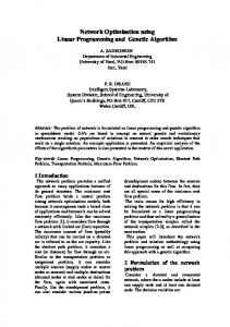
5.3. Real World Performance Real industrial CAD models are more challenging: models may include hundreds of thousands or even millions of entities. In this case, performance is potentially a serious problem. In real models, there are more types of entities, including subfeatures, and features are more complex than the simple ones used in earlier tests. All of these are big challenges for traditional algorithms. In this section, we show tests on several larger models to help assess the potential of our approach for industrial use. First we compare the performance of the approach in this paper with that of the method described in our previous work, using increasingly complex models of a carbine, switch and CPU heat sink (see Figs. 9–11); the features to be found were again open slots, blind slots, and through holes. Feature finding (see Table 3) took much less time than when using our previous approach for the CPU heat sink and switch. Similar times were achieved for the carbine, probably due to its simplicity. This is in agreement with our earlier experimental finding that the new approach has lower time complexity—it scales up better to larger models. These results are very 37

Figure 11: CPU heatsink

Model Number of edges Number of slots Unoptimized query Old translation (SQLite) New translation (PostgreSQL)

Carbine Switch CPU heatsink 84 330 2388 6 9 24 15 hours 50 ms 220 ms 6940 ms 47 ms 69 ms 107 ms

Table 3: Time taken to find slots in real models

encouraging, and show that the current approach can rapidly find features in models of realistic complexity. Feature finding took just 0.1 s even for the heatsink which has over 2000 edges. We have also performed further experiments on real industrial models to assess performance. Fig. 12 shows a moderately complex reducer model obtained from [44], with 17774 edges. It includes hundreds of open slots, blind slots, through-holes, and other features. Our feature recognizer can find such features in this model in a fraction of a second: see Table 4.

38

Figure 12: Reducer

Feature Number of features Time taken

Open slot 140 168 ms

Blind slot 146 176 ms

Throughhole 164 87 ms

Table 4: Time taken to find various features on a reducer model with 17774 edges

More complex features can be defined using subfeatures—features can often be decomposed into several similar sub-structures. Finding such substructures first and then combining them into a complete feature simplifies the writing of feature definitions. For example, we can define an adjacentpair-of-blind-slots feature, and seek it in the reducer model. This new feature comprises two round corner blind slots which are connected by short edges. We can first find the slot features (with 17 edges and 10 faces), and then determine which of those are adjacent and connected by short edges. Times taken for this task are given in Table 5, and again, are suitably low. More 39

generally, however, regularly structured features with arbitrary numbers of elements, such as a ring of holes, a gear, or a row of slots, are most easily defined recursively. This in turns needs a database which can handle recursive SQL queries; we intend to investigate such an approach in our future work. Feature Number of features Time taken

round corner bind slot 5 168 ms

adjacent slot pair 4 56 ms

Table 5: Time taken to find adjacent slot pairs in the reducer model

5.4. Lazy evaluation Lazy evaluation and predicate ordering are of greatest benefit when finding complex features which involve more than simple topological relationships and edge predicates such as convexity. We use the problem of finding features satisfying certain area constraints to illustrate the effectiveness of lazy evaluation. We compare results obtained by eager and lazy evaluation, CADfix being used to compute face areas. Results are cached in a temporary face area table linking face id and face area. We consider five alternative ways to find feature instances: • Eager evaluation (a). Pre-calculate and cache areas in a local table, and translate the corresponding constraint into a filter predicate in a WHERE clause. • Eager evaluation (b). Express area computations as remote CAD functions, translate constraints into filter predicates in WHERE clauses, and evaluate all area computations at execution time by calling CADfix. • Eager evaluation (c). Express area computations as remote CAD functions, and translate constraints into filter predicates in WHERE clauses. A local table is used to cache returned areas, so that CADfix is only asked to compute them once. • Lazy evaluation (a). Express area computations as remote CAD functions, translate them via HAVING clauses, and evaluate all area computations at execution time by calling CADfix.

40

• Lazy evaluation (b). Express area computations as remote CAD functions, translate them via HAVING clauses. A local table is used to cache returned areas, so that CADfix is only asked to compute them once. This leads, for example, to the following different ways of finding large through-hole features: 1 2 3 4 5 6 7 8 9 10 11 12 13 14 15 16 17 18 19 20 21 22 23 24 25 26 27 28 29 30 31 32 33 34 35 36 37 38 39

SELECT full_edge_e1 . edge AS e1 , full_edge_e2 . edge AS e2 , full_edge_e3 . edge AS e3 , full_edge_e4 . edge AS e4 , full_edge_e5 . edge AS e5 , full_edge_e6 . edge AS e6 , full_edge_e1 . face1 AS f1 , full_edge_e3 . face1 AS f2 , full_edge_e1 . face2 AS f3 , full_edge_e2 . face2 AS f4 FROM full_edge full_edge_e6 , full_edge full_edge_e5 , full_edge full_edge_e4 , full_edge full_edge_e3 , full_edge full_edge_e2 , full_edge full_edge_e1 , face_area fa , face_area fb WHERE full_edge_e1 . face1 = full_edge_e2 . face1 AND full_edge_e1 . face2 = full_edge_e3 . face2 AND full_edge_e1 . face2 = full_edge_e5 . face1 AND full_edge_e1 . face2 = full_edge_e6 . face2 AND full_edge_e2 . face2 = full_edge_e4 . face2 AND full_edge_e2 . face2 = full_edge_e5 . face2 AND full_edge_e2 . face2 = full_edge_e6 . face1 AND full_edge_e3 . face1 = full_edge_e4 . face1 AND full_edge_e3 . face2 = full_edge_e5 . face1 AND full_edge_e3 . face2 = full_edge_e6 . face2 AND full_edge_e4 . face2 = full_edge_e5 . face2 AND full_edge_e4 . face2 = full_edge_e6 . face1 AND full_edge_e1 . convexity =2 AND full_edge_e2 . convexity =2 AND full_edge_e3 . convexity =2 AND full_edge_e4 . convexity =2 AND full_edge_e5 . convexity =3 AND full_edge_e6 . convexity =3 AND full_edge_e3 . face1 < > full_edge_e2 . face2 AND full_edge_e3 . face1 < > full_edge_e1 . face2 AND full_edge_e3 . face1 < > full_edge_e1 . face1

41

40 41 42 43 44 45 46 47 48 49 50 51 52 53 54 55 56 57 58 59 60 61

AND AND AND AND AND AND AND AND AND AND AND AND AND AND AND AND AND AND AND AND AND AND

full_edge_e2 . face2 < > full_edge_e1 . face2 full_edge_e2 . face2 < > full_edge_e1 . face1 full_edge_e1 . face2 < > full_edge_e1 . face1 full_edge_e6 . edge < > full_edge_e5 . edge full_edge_e6 . edge < > full_edge_e4 . edge full_edge_e6 . edge < > full_edge_e3 . edge full_edge_e6 . edge < > full_edge_e2 . edge full_edge_e6 . edge < > full_edge_e1 . edge full_edge_e5 . edge < > full_edge_e4 . edge full_edge_e5 . edge < > full_edge_e3 . edge full_edge_e5 . edge < > full_edge_e2 . edge full_edge_e5 . edge < > full_edge_e1 . edge full_edge_e4 . edge < > full_edge_e3 . edge full_edge_e4 . edge < > full_edge_e2 . edge full_edge_e4 . edge < > full_edge_e1 . edge full_edge_e3 . edge < > full_edge_e2 . edge full_edge_e3 . edge < > full_edge_e1 . edge full_edge_e2 . edge < > full_edge_e1 . edge fa . face = full_edge_e1 . face2 fb . face = full_edge_e2 . face2 fa . area > 100 fb . area > 100; Listing 5: Eager evaluation (a)

1 2 3 4 5 6 7 8 9 10 11 12 13 14 15 16 17 18 19 20 21

SELECT full_edge_e1 . edge AS e1 , full_edge_e2 . edge AS e2 , full_edge_e3 . edge AS e3 , full_edge_e4 . edge AS e4 , full_edge_e5 . edge AS e5 , full_edge_e6 . edge AS e6 , full_edge_e1 . face1 AS f1 , full_edge_e3 . face1 AS f2 , full_edge_e1 . face2 AS f3 , full_edge_e2 . face2 AS f4 FROM full_edge full_edge_e6 , full_edge full_edge_e5 , full_edge full_edge_e4 , full_edge full_edge_e3 , full_edge full_edge_e2 , full_edge full_edge_e1 WHERE full_edge_e1 . face1 = full_edge_e2 . face1 AND full_edge_e1 . face2 = full_edge_e3 . face2 AND full_edge_e1 . face2 = full_edge_e5 . face1 AND full_edge_e1 . face2 = full_edge_e6 . face2 AND full_edge_e2 . face2 = full_edge_e4 . face2

42

22 23 24 25 26 27 28 29 30 31 32 33 34 35 36 37 38 39 40 41 42 43 44 45 46 47 48 49 50 51 52 53 54 55 56 57

AND AND AND AND AND AND AND AND AND AND AND AND AND AND AND AND AND AND AND AND AND AND AND AND AND AND AND AND AND AND AND AND AND AND AND AND

full_edge_e2 . face2 = full_edge_e5 . face2 full_edge_e2 . face2 = full_edge_e6 . face1 full_edge_e3 . face1 = full_edge_e4 . face1 full_edge_e3 . face2 = full_edge_e5 . face1 full_edge_e3 . face2 = full_edge_e6 . face2 full_edge_e4 . face2 = full_edge_e5 . face2 full_edge_e4 . face2 = full_edge_e6 . face1 full_edge_e1 . convexity =2 full_edge_e2 . convexity =2 full_edge_e3 . convexity =2 full_edge_e4 . convexity =2 full_edge_e5 . convexity =3 full_edge_e6 . convexity =3 full_edge_e3 . face1 < > full_edge_e2 . face2 full_edge_e3 . face1 < > full_edge_e1 . face2 full_edge_e3 . face1 < > full_edge_e1 . face1 full_edge_e2 . face2 < > full_edge_e1 . face2 full_edge_e2 . face2 < > full_edge_e1 . face1 full_edge_e1 . face2 < > full_edge_e1 . face1 full_edge_e6 . edge < > full_edge_e5 . edge full_edge_e6 . edge < > full_edge_e4 . edge full_edge_e6 . edge < > full_edge_e3 . edge full_edge_e6 . edge < > full_edge_e2 . edge full_edge_e6 . edge < > full_edge_e1 . edge full_edge_e5 . edge < > full_edge_e4 . edge full_edge_e5 . edge < > full_edge_e3 . edge full_edge_e5 . edge < > full_edge_e2 . edge full_edge_e5 . edge < > full_edge_e1 . edge full_edge_e4 . edge < > full_edge_e3 . edge full_edge_e4 . edge < > full_edge_e2 . edge full_edge_e4 . edge < > full_edge_e1 . edge full_edge_e3 . edge < > full_edge_e2 . edge full_edge_e3 . edge < > full_edge_e1 . edge full_edge_e2 . edge < > full_edge_e1 . edge calc_area ( full_edge_e1 . face2 ) >100 calc_area ( full_edge_e2 . face2 ) >100; Listing 6: Eager evaluation (b)

1 2 3 4 5 6 7

SELECT full_edge_e1 . edge full_edge_e2 . edge full_edge_e3 . edge full_edge_e4 . edge full_edge_e5 . edge full_edge_e6 . edge

AS AS AS AS AS AS

e1 , e2 , e3 , e4 , e5 , e6 ,

43

8 9 10 11 12

FROM

13 14 15 16 17 18 19 20 21 22 23 24 25 26 27 28 29 30 31 32 33 34 35 36 37 38 39 40 41 42 43 44 45 46 47 48 49 50 51 52

WHERE AND AND AND AND AND AND AND AND AND AND AND AND AND AND AND AND AND AND AND AND AND AND AND AND AND AND AND AND AND AND AND AND AND AND

full_edge_e1 . face1 AS f1 , full_edge_e3 . face1 AS f2 , full_edge_e1 . face2 AS f3 , full_edge_e2 . face2 AS f4 full_edge full_edge_e6 , full_edge full_edge_e5 , full_edge full_edge_e4 , full_edge full_edge_e3 , full_edge full_edge_e2 , full_edge full_edge_e1 full_edge_e1 . face1 = full_edge_e2 . face1 full_edge_e1 . face2 = full_edge_e3 . face2 full_edge_e1 . face2 = full_edge_e5 . face1 full_edge_e1 . face2 = full_edge_e6 . face2 full_edge_e2 . face2 = full_edge_e4 . face2 full_edge_e2 . face2 = full_edge_e5 . face2 full_edge_e2 . face2 = full_edge_e6 . face1 full_edge_e3 . face1 = full_edge_e4 . face1 full_edge_e3 . face2 = full_edge_e5 . face1 full_edge_e3 . face2 = full_edge_e6 . face2 full_edge_e4 . face2 = full_edge_e5 . face2 full_edge_e4 . face2 = full_edge_e6 . face1 full_edge_e1 . convexity =2 full_edge_e2 . convexity =2 full_edge_e3 . convexity =2 full_edge_e4 . convexity =2 full_edge_e5 . convexity =3 full_edge_e6 . convexity =3 full_edge_e3 . face1 < > full_edge_e2 . face2 full_edge_e3 . face1 < > full_edge_e1 . face2 full_edge_e3 . face1 < > full_edge_e1 . face1 full_edge_e2 . face2 < > full_edge_e1 . face2 full_edge_e2 . face2 < > full_edge_e1 . face1 full_edge_e1 . face2 < > full_edge_e1 . face1 full_edge_e6 . edge < > full_edge_e5 . edge full_edge_e6 . edge < > full_edge_e4 . edge full_edge_e6 . edge < > full_edge_e3 . edge full_edge_e6 . edge < > full_edge_e2 . edge full_edge_e6 . edge < > full_edge_e1 . edge full_edge_e5 . edge < > full_edge_e4 . edge full_edge_e5 . edge < > full_edge_e3 . edge full_edge_e5 . edge < > full_edge_e2 . edge full_edge_e5 . edge < > full_edge_e1 . edge full_edge_e4 . edge < > full_edge_e3 . edge full_edge_e4 . edge < > full_edge_e2 . edge

44

53 54 55 56 57 58

AND AND AND AND AND AND

full_edge_e4 . edge < > full_edge_e1 . edge full_edge_e3 . edge < > full_edge_e2 . edge full_edge_e3 . edge < > full_edge_e1 . edge full_edge_e2 . edge < > full_edge_e1 . edge get_area ( full_edge_e1 . face2 ) >100 get_area ( full_edge_e2 . face2 ) >100; Listing 7: Eager evaluation (c)

In this query, the remote CAD predicate get_area is defined as: 1 2 3 4 5 6 7 8 9 10 11

CREATE or replace FUNCTION get_area ( face integer ) RETURNS float AS $$ DECLARE RSLT float ; BEGIN SELECT area into rslt FROM face_area WHERE face_area . face = $1 ; IF NOT FOUND THEN rslt := calc_area ( $1 ) ; INSERT INTO face_area VALUES ( $1 , rslt ) ; END IF ; return rslt ; END ; $$ LANGUAGE plpgsql ; Listing 8: Lazy cache function

1 2 3 4 5 6 7 8 9 10 11 12 13 14 15 16 17 18 19 20 21 22

SELECT full_edge_e1 . edge AS e1 , full_edge_e2 . edge AS e2 , full_edge_e3 . edge AS e3 , full_edge_e4 . edge AS e4 , full_edge_e5 . edge AS e5 , full_edge_e6 . edge AS e6 , full_edge_e1 . face1 AS f1 , full_edge_e3 . face1 AS f2 , full_edge_e1 . face2 AS f3 , full_edge_e2 . face2 AS f4 FROM full_edge full_edge_e6 , full_edge full_edge_e5 , full_edge full_edge_e4 , full_edge full_edge_e3 , full_edge full_edge_e2 , full_edge full_edge_e1 WHERE full_edge_e1 . face1 = full_edge_e2 . face1 AND full_edge_e1 . face2 = full_edge_e3 . face2 AND full_edge_e1 . face2 = full_edge_e5 . face1 AND full_edge_e1 . face2 = full_edge_e6 . face2 AND full_edge_e2 . face2 = full_edge_e4 . face2

45

23 24 25 26 27 28 29 30 31 32 33 34 35 36 37 38 39 40 41 42 43 44 45 46 47 48 49 50 51 52 53 54 55 56 57 58 59 60 61 62 63 64 65 66 67

AND AND AND AND AND AND AND AND AND AND AND AND AND AND AND AND AND AND AND AND AND AND AND AND AND AND AND AND AND AND AND AND AND AND GROUP

full_edge_e2 . face2 = full_edge_e5 . face2 full_edge_e2 . face2 = full_edge_e6 . face1 full_edge_e3 . face1 = full_edge_e4 . face1 full_edge_e3 . face2 = full_edge_e5 . face1 full_edge_e3 . face2 = full_edge_e6 . face2 full_edge_e4 . face2 = full_edge_e5 . face2 full_edge_e4 . face2 = full_edge_e6 . face1 full_edge_e1 . convexity =2 full_edge_e2 . convexity =2 full_edge_e3 . convexity =2 full_edge_e4 . convexity =2 full_edge_e5 . convexity =3 full_edge_e6 . convexity =3 full_edge_e3 . face1 < > full_edge_e2 . face2 full_edge_e3 . face1 < > full_edge_e1 . face2 full_edge_e3 . face1 < > full_edge_e1 . face1 full_edge_e2 . face2 < > full_edge_e1 . face2 full_edge_e2 . face2 < > full_edge_e1 . face1 full_edge_e1 . face2 < > full_edge_e1 . face1 full_edge_e6 . edge < > full_edge_e5 . edge full_edge_e6 . edge < > full_edge_e4 . edge full_edge_e6 . edge < > full_edge_e3 . edge full_edge_e6 . edge < > full_edge_e2 . edge full_edge_e6 . edge < > full_edge_e1 . edge full_edge_e5 . edge < > full_edge_e4 . edge full_edge_e5 . edge < > full_edge_e3 . edge full_edge_e5 . edge < > full_edge_e2 . edge full_edge_e5 . edge < > full_edge_e1 . edge full_edge_e4 . edge < > full_edge_e3 . edge full_edge_e4 . edge < > full_edge_e2 . edge full_edge_e4 . edge < > full_edge_e1 . edge full_edge_e3 . edge < > full_edge_e2 . edge full_edge_e3 . edge < > full_edge_e1 . edge full_edge_e2 . edge < > full_edge_e1 . edge BY full_edge_e1 . edge , full_edge_e2 . edge , full_edge_e3 . edge , full_edge_e4 . edge , full_edge_e5 . edge , full_edge_e6 . edge , full_edge_e1 . face1 , full_edge_e3 . face1 , full_edge_e1 . face2 , full_edge_e2 . face2 HAVING calc_area ( full_edge_e1 . face2 ) >100

46

68

AND calc_area ( full_edge_e2 . face2 ) >100; Listing 9: Lazy evaluation (a)

1 2 3 4 5 6 7 8 9 10 11 12 13 14 15 16 17 18 19 20 21 22 23 24 25 26 27 28 29 30 31 32 33 34 35 36 37 38 39 40 41 42

SELECT full_edge_e1 . edge AS e1 , full_edge_e2 . edge AS e2 , full_edge_e3 . edge AS e3 , full_edge_e4 . edge AS e4 , full_edge_e5 . edge AS e5 , full_edge_e6 . edge AS e6 , full_edge_e1 . face1 AS f1 , full_edge_e3 . face1 AS f2 , full_edge_e1 . face2 AS f3 , full_edge_e2 . face2 AS f4 FROM full_edge full_edge_e6 , full_edge full_edge_e5 , full_edge full_edge_e4 , full_edge full_edge_e3 , full_edge full_edge_e2 , full_edge full_edge_e1 WHERE full_edge_e1 . face1 = full_edge_e2 . face1 AND full_edge_e1 . face2 = full_edge_e3 . face2 AND full_edge_e1 . face2 = full_edge_e5 . face1 AND full_edge_e1 . face2 = full_edge_e6 . face2 AND full_edge_e2 . face2 = full_edge_e4 . face2 AND full_edge_e2 . face2 = full_edge_e5 . face2 AND full_edge_e2 . face2 = full_edge_e6 . face1 AND full_edge_e3 . face1 = full_edge_e4 . face1 AND full_edge_e3 . face2 = full_edge_e5 . face1 AND full_edge_e3 . face2 = full_edge_e6 . face2 AND full_edge_e4 . face2 = full_edge_e5 . face2 AND full_edge_e4 . face2 = full_edge_e6 . face1 AND full_edge_e1 . convexity =2 AND full_edge_e2 . convexity =2 AND full_edge_e3 . convexity =2 AND full_edge_e4 . convexity =2 AND full_edge_e5 . convexity =3 AND full_edge_e6 . convexity =3 AND full_edge_e3 . face1 < > full_edge_e2 . face2 AND full_edge_e3 . face1 < > full_edge_e1 . face2 AND full_edge_e3 . face1 < > full_edge_e1 . face1 AND full_edge_e2 . face2 < > full_edge_e1 . face2 AND full_edge_e2 . face2 < > full_edge_e1 . face1 AND full_edge_e1 . face2 < > full_edge_e1 . face1 AND full_edge_e6 . edge < > full_edge_e5 . edge

47

43 44 45 46 47 48 49 50 51 52 53 54 55 56 57 58 59 60 61 62 63 64 65 66 67 68

AND AND AND AND AND AND AND AND AND AND AND AND AND AND GROUP

full_edge_e6 . edge < > full_edge_e4 . edge full_edge_e6 . edge < > full_edge_e3 . edge full_edge_e6 . edge < > full_edge_e2 . edge full_edge_e6 . edge < > full_edge_e1 . edge full_edge_e5 . edge < > full_edge_e4 . edge full_edge_e5 . edge < > full_edge_e3 . edge full_edge_e5 . edge < > full_edge_e2 . edge full_edge_e5 . edge < > full_edge_e1 . edge full_edge_e4 . edge < > full_edge_e3 . edge full_edge_e4 . edge < > full_edge_e2 . edge full_edge_e4 . edge < > full_edge_e1 . edge full_edge_e3 . edge < > full_edge_e2 . edge full_edge_e3 . edge < > full_edge_e1 . edge full_edge_e2 . edge < > full_edge_e1 . edge BY full_edge_e1 . edge , full_edge_e2 . edge , full_edge_e3 . edge , full_edge_e4 . edge , full_edge_e5 . edge , full_edge_e6 . edge , full_edge_e1 . face1 , full_edge_e3 . face1 , full_edge_e1 . face2 , full_edge_e2 . face2 HAVING get_area ( full_edge_e1 . face2 ) > 100 AND get_area ( full_edge_e2 . face2 ) >100; Listing 10: Lazy evaluation (b)

We performed the following three experiments to determine the impact of lazy evaluation, Table 6 gives the numbers of features found and Table 7 gives the times taken to find these features in the reducer model in Fig. 12. Task 1. Find open slots with side face area greater than 20, and bottom face area greater than 2; Task 2. Find all through-holes with side face area less than 550 and bore area smaller than 50; Task 3. Find all through-holes with cylindrical faces area greater than 100; As Table 7 shows, the lazy evaluation approach (b) achieved the best performance in each case, being about 6 to 8 times faster than eager evaluation approach (a), much better than eager evaluation approaches (b) and (c). It 48

Task Number of features, any size Number of features, specified size

Task 1 140 35

Task 2 164 18

Task 3 164 142

Table 6: Feature finding results for various tasks

Experiment Eager evaluation (a) Eager evaluation (b) Eager evaluation (c) Lazy evaluation (a) Lazy evaluation (b)

Task 1 1215.8 40310.6 11398.9 228.3 162.7

Task 2 1322.9 51285.7 15471.4 1278.6 209.7

Task 3 1313.8 53308.9 14426.2 400.7 155.6

Table 7: Feature finding times (in milliseconds) for the reducer models, using different evaluation strategies, and different tasks.

is also about twice as fast as lazy evaluation approach (a). Using eager evaluation (a) takes about the same time for each task, because of the similar procedure—first calculate areas of all faces, cache them in a local table and then perform a filter based query; time is dominated by the area calculations. Eager evaluation (b) is the slowest approach: the area of each face is evaluated multiple times. Eager evaluation (c) is better, as caching means that areas are only computed once. For the same reason, lazy evaluation approach (b) performs better than lazy evaluation approach (a). 5.5. Predicate ordering For complex models, when multiple time consuming predicates must be evaluated, correctly ordering them can improve performance. In this section, we show further experiments which not only use lazy evaluation, but also plan execution order based on selectivity combined with average times for predicate evaluation. Determining average times and selectivity requires offline training on a large model set. For this, we used 826 real industrial models of CPU heat sinks downloaded from micforg [45]. Examples of these models are shown in Fig. 13. The model in which features are to be found is shown in Fig 14, which, like other CPU heat sinks, includes a large base and fins of several different sizes. Detailed fin structure is illustrated in Fig 15. Each fin is composed of two cylindrical faces with two tangentially connected side faces, a top face and a bottom edge loop. 49

Figure 13: Examples from CPU heatsink training set

The feature recognition task here is to find small fins, defined as fins whose side face area is between 10 and 20 square units, and whose top face has perimeter between 18.5 and 18.7 units. This requires the predicates 1 2

area_in_range ( full_edge_e4 . face2 , 10 , 20) p eri me te r_ in _r an ge ( full_edge_e1 . face1 , 18.5 , 18.7) ;

In our feature finder, these range predicates are translated so as to be processed in PostgreSQL using lazy evaluation with caching, where in turn the function calc_area is a remote CAD function call to CADfix. 1

CREATE OR REPLACE FUNCTION area_in_range ( face int , lv float ,

50

Figure 14: Model in which we wish to find small fins

2 3 4 5 6 7 8 9 10 11 12 13 14

hv float ) RETURNS boolean AS $$ DECLARE RSLT float ; val boolean ; BEGIN SELECT area INTO rslt FROM face_area WHERE face_area . face = $1 ; IF NOT FOUND THEN rslt := calc_area ( $1 ) ; INSERT INTO face_area VALUES ( $1 , rslt ) ; END IF ; RETURN (( rslt > $2 ) and ( rslt < $3 ) ) ; END ; $$ LANGUAGE plpgsql ;

To estimate the cost and selectivity of the area and perimeter functions, offline training is performed on the set of training models. The area and perimeter distributions are shown in Figs. 16 and 17 respectively. Average times to compute these properties, and their selectivity for the particular ranges of values used in the test, are given in Table 8. The target query used to find small fins is as follows, where the two 51

Figure 15: Fin detail

Predicate area in range perimeter in range

average execution time 1 ms 0.003 ms

average selectivity 0.2231 0.0084

Table 8: Selectivity and cost of target predicates

predicates in the HAVING clause are the ones being considered for reordering: 1 2 3 4 5 6 7 8 9 10 11 12 13

SELECT full_edge_e1 . edge AS e1 , full_edge_e2 . edge AS e2 , full_edge_e3 . edge AS e3 , full_edge_e4 . edge AS e4 , full_edge_e5 . edge AS e5 , full_edge_e6 . edge AS e6 , full_edge_e7 . edge AS e7 , full_edge_e8 . edge AS e8 , full_edge_e9 . edge AS e9 , full_edge_e10 . edge AS e10 , full_edge_e11 . edge AS e11 , full_edge_e12 . edge AS e12 , full_edge_e1 . face1 AS f1 ,

52

4

7

x 10

6

5

Counts

4

3

2

1

0 −6

−5

−4

−3

−2 −1 log (area/mean)

0

1

2

10

Figure 16: Histogram of face areas for training model dataset

14 15 16 17 18 19 20 21 22 23 24 25

full_edge_e1 . face2 AS f2 , full_edge_e4 . face2 AS f3 , full_edge_e3 . face2 AS f4 , full_edge_e2 . face2 AS f5 , full_edge_e9 . face2 AS f6 FROM full_edge full_edge_e12 , full_edge full_edge_e11 , full_edge full_edge_e10 , full_edge full_edge_e9 , full_edge full_edge_e8 , full_edge full_edge_e7 , full_edge full_edge_e6 ,

53

3

4

12

x 10

10

Counts

8

6

4

2

0 −3

−2.5

−2

−1.5

−1 −0.5 log10(perimeter/mean)

0

0.5

1

Figure 17: Histogram of face perimeters for training model dataset

26 27 28 29 30 31 32 33 34 35 36 37

full_edge full_edge_e5 , full_edge full_edge_e4 , full_edge full_edge_e3 , full_edge full_edge_e2 , full_edge full_edge_e1 WHERE full_edge_e1 . face1 = full_edge_e2 . face1 AND full_edge_e1 . face1 = full_edge_e3 . face1 AND full_edge_e1 . face1 = full_edge_e4 . face1 AND full_edge_e1 . face2 = full_edge_e5 . face1 AND full_edge_e1 . face2 = full_edge_e6 . face1 AND full_edge_e1 . face2 = full_edge_e9 . face1 AND full_edge_e2 . face1 = full_edge_e3 . face1

54

1.5

38 39 40 41 42 43 44 45 46 47 48 49 50 51 52 53 54 55 56 57 58 59 60 61 62 63 64 65 66 67 68 69 70 71 72 73 74 75 76 77 78 79 80 81 82

AND AND AND AND AND AND AND AND AND AND AND AND AND AND AND AND AND AND AND AND AND AND AND AND AND AND AND AND AND AND AND AND AND AND AND AND AND AND AND AND AND AND AND AND AND

full_edge_e2 . face1 = full_edge_e4 . face1 full_edge_e2 . face2 = full_edge_e5 . face2 full_edge_e2 . face2 = full_edge_e8 . face2 full_edge_e2 . face2 = full_edge_e12 . face2 full_edge_e3 . face1 = full_edge_e4 . face1 full_edge_e3 . face2 = full_edge_e7 . face2 full_edge_e3 . face2 = full_edge_e8 . face1 full_edge_e3 . face2 = full_edge_e11 . face1 full_edge_e4 . face2 = full_edge_e6 . face2 full_edge_e4 . face2 = full_edge_e7 . face1 full_edge_e4 . face2 = full_edge_e10 . face2 full_edge_e5 . face1 = full_edge_e6 . face1 full_edge_e5 . face2 = full_edge_e8 . face2 full_edge_e5 . face1 = full_edge_e9 . face1 full_edge_e5 . face2 = full_edge_e12 . face2 full_edge_e6 . face2 = full_edge_e7 . face1 full_edge_e6 . face1 = full_edge_e9 . face1 full_edge_e6 . face2 = full_edge_e10 . face2 full_edge_e7 . face2 = full_edge_e8 . face1 full_edge_e7 . face1 = full_edge_e10 . face2 full_edge_e7 . face2 = full_edge_e11 . face1 full_edge_e8 . face1 = full_edge_e11 . face1 full_edge_e8 . face2 = full_edge_e12 . face2 full_edge_e9 . face2 = full_edge_e10 . face1 full_edge_e9 . face2 = full_edge_e11 . face2 full_edge_e9 . face2 = full_edge_e12 . face1 full_edge_e10 . face1 = full_edge_e11 . face2 full_edge_e10 . face1 = full_edge_e12 . face1 full_edge_e11 . face2 = full_edge_e12 . face1 full_edge_e1 . convexity =2 full_edge_e2 . convexity =2 full_edge_e3 . convexity =2 full_edge_e4 . convexity =2 full_edge_e5 . convexity =3 full_edge_e6 . convexity =3 full_edge_e7 . convexity =3 full_edge_e8 . convexity =3 full_edge_e9 . convexity =1 full_edge_e10 . convexity =1 full_edge_e11 . convexity =1 full_edge_e12 . convexity =1 full_edge_e12 . edge < > full_edge_e11 . edge full_edge_e12 . edge < > full_edge_e10 . edge full_edge_e12 . edge < > full_edge_e9 . edge full_edge_e12 . edge < > full_edge_e8 . edge

55

83 84 85 86 87 88 89 90 91 92 93 94 95 96 97 98 99 100 101 102 103 104 105 106 107 108 109 110 111 112 113 114 115 116 117 118 119 120 121 122 123 124 125 126 127

AND AND AND AND AND AND AND AND AND AND AND AND AND AND AND AND AND AND AND AND AND AND AND AND AND AND AND AND AND AND AND AND AND AND AND AND AND AND AND AND AND AND AND AND AND

full_edge_e12 . edge < > full_edge_e7 . edge full_edge_e12 . edge < > full_edge_e6 . edge full_edge_e12 . edge < > full_edge_e5 . edge full_edge_e12 . edge < > full_edge_e4 . edge full_edge_e12 . edge < > full_edge_e3 . edge full_edge_e12 . edge < > full_edge_e2 . edge full_edge_e12 . edge < > full_edge_e1 . edge full_edge_e11 . edge < > full_edge_e10 . edge full_edge_e11 . edge < > full_edge_e9 . edge full_edge_e11 . edge < > full_edge_e8 . edge full_edge_e11 . edge < > full_edge_e7 . edge full_edge_e11 . edge < > full_edge_e6 . edge full_edge_e11 . edge < > full_edge_e5 . edge full_edge_e11 . edge < > full_edge_e4 . edge full_edge_e11 . edge < > full_edge_e3 . edge full_edge_e11 . edge < > full_edge_e2 . edge full_edge_e11 . edge < > full_edge_e1 . edge full_edge_e10 . edge < > full_edge_e9 . edge full_edge_e10 . edge < > full_edge_e8 . edge full_edge_e10 . edge < > full_edge_e7 . edge full_edge_e10 . edge < > full_edge_e6 . edge full_edge_e10 . edge < > full_edge_e5 . edge full_edge_e10 . edge < > full_edge_e4 . edge full_edge_e10 . edge < > full_edge_e3 . edge full_edge_e10 . edge < > full_edge_e2 . edge full_edge_e10 . edge < > full_edge_e1 . edge full_edge_e9 . edge < > full_edge_e8 . edge full_edge_e9 . edge < > full_edge_e7 . edge full_edge_e9 . edge < > full_edge_e6 . edge full_edge_e9 . edge < > full_edge_e5 . edge full_edge_e9 . edge < > full_edge_e4 . edge full_edge_e9 . edge < > full_edge_e3 . edge full_edge_e9 . edge < > full_edge_e2 . edge full_edge_e9 . edge < > full_edge_e1 . edge full_edge_e8 . edge < > full_edge_e7 . edge full_edge_e8 . edge < > full_edge_e6 . edge full_edge_e8 . edge < > full_edge_e5 . edge full_edge_e8 . edge < > full_edge_e4 . edge full_edge_e8 . edge < > full_edge_e3 . edge full_edge_e8 . edge < > full_edge_e2 . edge full_edge_e8 . edge < > full_edge_e1 . edge full_edge_e7 . edge < > full_edge_e6 . edge full_edge_e7 . edge < > full_edge_e5 . edge full_edge_e7 . edge < > full_edge_e4 . edge full_edge_e7 . edge < > full_edge_e3 . edge

56

128 129 130 131 132 133 134 135 136 137 138 139 140 141 142 143 144 145 146 147 148 149 150 151 152 153 154 155 156 157 158 159 160 161 162 163 164 165 166

AND AND AND AND AND AND AND AND AND AND AND AND AND AND AND AND AND AND AND GROUP

full_edge_e7 . edge < > full_edge_e2 . edge full_edge_e7 . edge < > full_edge_e1 . edge full_edge_e6 . edge < > full_edge_e5 . edge full_edge_e6 . edge < > full_edge_e4 . edge full_edge_e6 . edge < > full_edge_e3 . edge full_edge_e6 . edge < > full_edge_e2 . edge full_edge_e6 . edge < > full_edge_e1 . edge full_edge_e5 . edge < > full_edge_e4 . edge full_edge_e5 . edge < > full_edge_e3 . edge full_edge_e5 . edge < > full_edge_e2 . edge full_edge_e5 . edge < > full_edge_e1 . edge full_edge_e4 . edge < > full_edge_e3 . edge full_edge_e4 . edge < > full_edge_e2 . edge full_edge_e4 . edge < > full_edge_e1 . edge full_edge_e3 . edge < > full_edge_e2 . edge full_edge_e3 . edge < > full_edge_e1 . edge full_edge_e2 . edge < > full_edge_e1 . edge face_geometry_is ( full_edge_e1 . face2 ,2006) face_geometry_is ( full_edge_e3 . face2 ,2006) BY full_edge_e1 . edge , full_edge_e2 . edge , full_edge_e3 . edge , full_edge_e4 . edge , full_edge_e5 . edge , full_edge_e6 . edge , full_edge_e7 . edge , full_edge_e8 . edge , full_edge_e9 . edge , full_edge_e10 . edge , full_edge_e11 . edge , full_edge_e12 . edge , full_edge_e1 . face1 , full_edge_e1 . face2 , full_edge_e4 . face2 , full_edge_e3 . face2 , full_edge_e2 . face2 , full_edge_e9 . face2 HAVING area_in_range ( full_edge_e4 . face2 , 10 , 20) AND pe ri me te r_i n_ ra ng e ( full_edge_e1 . face1 , 18.5 , 18.7) ; Listing 11: Query to find small fins

We compared results obtained using our system based on the PostgreSQL engine with lazy evaluation, with and without predicate reordering. The test was repeated 100 times to give an averaged performance result. Each time the PostgreSQL server was restarted, warmed up and the OS caches (pagecache, 57

Method without reordering with reordering

area-perimeter 498 ms 392 ms

perimeter-area 393 ms 392 ms

Table 9: Average feature finding times with and without predicate reordering optimization

dentries and inodes) were cleared. For both versions, we timed the SQL query with the predicates given in either possible order: area then perimeter, or perimeter then area. With reordering, the query planner always chooses the predicate ordering perimeter then area, whichever ordering the predicates are initially provided in: the much higher cost of computing areas compared to perimeters far outweighs the differences in selectivity. Without reordering, predicates are simply executed in the sequence given. Fig. 18 give the times taken to find features in each of the 100 runs in each case, using the different strategies. Without reordering, the approaches take different times according to which predicate is evaluated first. Computing area first, most runs take 350–400 ms, while if perimeter is computed first, most runs take 490–530 ms. However, if reordering is used, no matter how the predicates are ordered in the original definition, the times taken in both cases have closely similar ranges and distributions. Average times are given in Table 9. As expected, the optimizer-chosen perimeter-then-area ordering is faster than the alternative area-then-perimeter ordering. The overhead required to perform the selectivity calculation is negligible. As effective translation and lazy evaluation already improve performance greatly, predicate ordering only makes a worthwhile difference for large models. Most of the time spent is running the query itself, rather than the CAD computations, so the saving is not much (21% in this case). Nevertheless, for other more complex predicates that the CAD modeller takes longer to process, the savings could be greater. 6. Conclusions This paper has shown that a declarative approach can find simple features in large scale CAD models in a fraction of a second. The key to this performance lies in database optimization techniques. Our particular contributions here are: (i) a novel approach to translating declarative feature definitions into SQL queries, with improved performance over our earlier work, (ii) use 58

Time taken between 350 and 400 ms Time taken between 400 and 450 ms Time taken between 450 and 490 ms Time taken between 490 and 530 ms 1 0.9 0.8

Fraction

0.7 0.6 0.5 0.4 0.3 0.2 0.1 0

NA

NP

RA

RP

Time taken between 350 and 400 ms Time taken between 400 and 450 ms Time taken between 450 and 490 ms Time taken between 490 and 530 ms 1 Figure 18: Times taken for for each of 100 runs. N = No reordering of predicates. R = 0.9of predicates. A = Area first. P = Perimeter first. Reordering 0.8

Fraction

of lazy evaluation to avoid computing complex predicates whose results are 0.7 and (iii) use of selectivity to reorder query processing for further not needed, minor improvements. 0.6 This work has demonstrated that it is possible to build an efficient, extensible,0.5 feature recognition system based on declarative feature definitions. Use is made of mature database query optimization technology to achieve 0.4 high performance, and indeed linear complexity for simple features. 0.3

Acknowledgements 0.2

This work was supported by Framework Programme 7 Initial Training Network0.1 Funding under Grant No. 289361. The authors would also like to 0

NA

NP 59

RA

RP

thank to Henry Bucklow and others from ITI TranscenData who provided CADfix software, CADfix API training and models. References [1] H. Zhu, C. Menq, B-rep model simplification by automatic fillet/round suppressing for efficient automatic feature recognition, Computer-Aided Design 34 (2002) 109–123. [2] M. M¨antyl¨a, D. Nau, J. Shah, Challenges in feature-based manufacturing research, Communications of the ACM 39 (1996) 77–85. [3] J. Han, M. Pratt, W. C. Regli, Manufacturing feature recognition from solid models: a status report, IEEE Trans. Robotics and Automation 16 (2000) 782–796. [4] B. Babic, N. Nesic, Z. Miljkovic, A review of automated feature recognition with rule-based pattern recognition, Computers in Industry 59 (2008) 321–337. [5] K. Lee, C. G. Armstrong, M. A. Price, J. Lamont, A small feature suppression/unsuppression system for preparing B-rep models for analysis, in: Proc. 2005 ACM Symp. Solid and Physical Modeling, ACM, pp. 113–124. [6] S. Gao, W. Zhao, H. Lin, F. Yang, X. Chen, Feature suppression based CAD mesh model simplification, Computer-Aided Design 42 (2010) 1178–1188. [7] M. Li, B. Zhang, R. R. Martin, Second-order defeaturing error estimation for multiple boundary features, Int. J. Numerical Methods in Engineering 100 (2014) 321–346. [8] H. L. Lockett, M. D. Guenov, Graph-based feature recognition for injection moulding based on a mid-surface approach, Computer-Aided Design 37 (2005) 251–262. [9] P. Gibson, H. Ismail, M. Sabin, K. Hon, Interactive programmable feature recogniser, CIRP Annals on Manufacturing Technology 46 (1997) 407–410. 60

[10] P. Gibson, H. Ismail, M. Sabin, Optimisation approaches in feature recognition, Int. J. Machine Tools and Manufacture 39 (1999) 805–821. [11] Z. Niu, R. R. Martin, M. Sabin, F. C. Langbein, H. Bucklow, Applying database optimization technologies to feature recognition in CAD, Computer-Aided Design and Applications (2014) 1–10. [12] H. Garcia-Molina, J. D. Ullman, J. Widom, Database system implementation, Prentice Hall, 2000. [13] L. K. Kyprianou, Shape classification in computer-aided design., Ph.D. thesis, University of Cambridge, 1980. [14] M. Marefat, R. Kashyap, Geometric reasoning for recognition of threedimensional object features, IEEE Trans. Pattern Analysis and Machine Intelligence 12 (1990) 949–965. [15] M. C. Fields, D. C. Anderson, Fast feature extraction for machining applications, Computer-Aided Design 26 (1994) 803–813. [16] J. J. Shah, D. Anderson, Y. S. Kim, S. Joshi, A discourse on geometric feature recognition from CAD models, J. Computing and Information Science in Engineering 1 (2001) 41–51. [17] A. Verma, S. Rajotia, Feature vector: a graph-based feature recognition methodology, Int. J. Production Research 42 (2004) 3219–3234. [18] T. Laakko, M. M¨antyl¨a, A feature definition language for bridging solids and features, in: Proc. 2nd ACM Symp. Solid Modeling and Applications, ACM, pp. 333–342. [19] H. K. Miao, N. Sridharan, J. J. Shah, CAD-CAM integration using machining features, Int. J. Computer Integrated Manufacturing 15 (2002) 296–318. [20] R. Sonthi, G. Kunjur, R. Gadh, Shape feature determination usiang the curvature region representation, in: Proc. 4th ACM Symposium on Solid Modeling and Applications, ACM, pp. 285–296. [21] G. Little, D. E. Clark, J. R. Corney, J. Tuttle, Delta-volume decomposition for multi-sided components, Computer-Aided Design 30 (1998) 695–705. 61

[22] X.-F. Cui, S.-M. Gao, G.-P. Zhou, An efficient algorithm for recognizing and suppressing blend features, Computer Integrated Manufacturing Systems 10 (2004) 77–82. [23] A. Dixon, J. J. Shah, Assembly feature tutor and recognition algorithms based on mating face pairs, Computer-Aided Design and Applications 7 (2010) 319–333. [24] J. Melton, Understanding the new SQL: a complete guide, Morgan Kaufmann, 1993. [25] Y. E. Ioannidis, Query optimization, ACM Computing Surveys 28 (1996) 121–123. [26] S. Chaudhuri, An overview of query optimization in relational systems, in: Proc. 17th ACM SIGACT-SIGMOD-SIGART Symp. Principles of Database Systems, ACM, pp. 34–43. [27] A. Rosenthal, C. Galindo-Legaria, Query graphs, implementing trees, and freely-reorderable outerjoins, ACM SIGMOD Record 19 (1990) 291–299. [28] S. Chaudhuri, K. Shim, An overview of cost-based optimization of queries with aggregates, IEEE Data Engineering Bulletin 18 (1995) 3–9. [29] D. R. Hipp, The SQLite query planner, https://www.sqlite.org/ optoverview.html, 2015. Retrieved 11 March 2015. [30] The PostgreSQL Global Development Group, PostgreSQL, http:// www.postgresql.org/about/, 2015. Retrieved 11 March 2015. [31] D. K. Burleson, Oracle tuning: the definitive reference, Rampant TechPress, 2010. [32] P. DuBois, MySQL (Developer’s Library), Sams, 2005. [33] B. Momjian, Explaining the PostgreSQL query optimizer, http:// pgday.ru/files/pgmaster14/bruce.momjian.optimizer.pdf, 2012. Retrieved 11 March 2015.

62

[34] P. Gibson, H. Ismail, M. Sabin, A feature recognition project, in: Product Modeling for Computer Integrated Design and Manufacture, Chapman & Hall, Ltd., pp. 179–190. [35] P. Spiby, D. Schenck, EXPRESS language reference manual, TC184/SC4 Document N 14 (1991).

ISO

[36] J. M. Hellerstein, M. Stonebraker, Predicate Migration: Optimizing Queries with Expensive Predicates, ACM, 1993. [37] B. Momjian, PostgreSQL: Introduction and Concepts, Addison-Wesley New York, 2001. [38] E. Geschwinde, H.-J. Sch¨onig, PostgreSQL Developer’s Handbook, Sams Publishing, 2002. [39] ITI Transcendata, CADfix, http://www.transcendata.com/ products/cadfix, 2015. Retrieved 11 March 2015. [40] G. Butlin, C. Stops, CAD data repair, in: 5th Int. Meshing Roundtable, pp. 7–12. [41] G. Graefe, The value of merge-join and hash-join in SQL Server, in: VLDB, pp. 250–253. [42] P. Garcia, H. F. Korth, Database hash-join algorithms on multithreaded computer architectures, in: Proc. 3rd Conf. Computing Frontiers, ACM, pp. 241–252. [43] The PostgreSQL Global Development Group, PostgreSQL statistical information, http://www.postgresql.org/docs/9.1/static/ view-pg-stats.html, 2015. Retrieved 11 March 2015. [44] GrabCAD, GrabCAD Free CAD Models, https://grabcad.com/ library, 2015. Retrieved 11 March 2015. [45] A. C. Ltd, Cpu heat sink, http://www.micforg.co.jp/en, 2015. Retrieved 18 March 2015.

63