1 Computer Science Department, Carnegie Mellon University. 5000 Forbes Avenue, Pittsburgh, PA 15213, USA. {jha|emc}@cs.cmu.edu. 2 ECE Department ...
Reachability for Linear Hybrid Automata Using Iterative Relaxation Abstraction Sumit K. Jha1 , Bruce H. Krogh2 , James E. Weimer2 , Edmund M. Clarke1 1
Computer Science Department, Carnegie Mellon University 5000 Forbes Avenue, Pittsburgh, PA 15213, USA {jha|emc}@cs.cmu.edu 2 ECE Department, Carnegie Mellon University 5000 Forbes Avenue, Pittsburgh, PA15213, USA {krogh| jweimer}@ece.cmu.edu ⋆⋆
Abstract. Procedures for analysis of linear hybrid automata (LHA) do not scale well with the number of continuous state variables in the model. This paper introduces iterative relaxation abstraction (IRA), a new method for reachability analysis of LHA that aims to improve scalability by combining the capabilities of current tools for analysis of lowdimensional LHA with the power of linear programming (LP) for large numbers of constraints and variables. IRA is inspired by the success of counterexample guided abstraction refinement (CEGAR) techniques in verification of discrete systems. On each iteration, a low-dimensional LHA called a relaxation abstraction is constructed using a subset of the continuous variables from the original LHA. Hybrid system reachability analysis then generates a regular language called the discrete path abstraction representing all possible counterexamples (paths to the bad locations) in the relaxation abstraction. If the discrete path abstraction is non-empty, a particular counterexample is selected and LP infeasibility analysis determines if the counterexample is spurious using the constraints along the path from the original high-dimensional LHA. If the counterexample is spurious, LP techniques identify an irreducible infeasible subset (IIS) of constraints from which the set of continuous variables is selected for the the construction of the next relaxation abstraction. IRA stops if the discrete path abstraction is empty or a legitimate counterexample is found. The effectiveness of the approach is illustrated with an example. ⋆⋆
This research was sponsored by the National Science Foundation under grant nos. CNS-0411152, CCF-0429120, CCR-0121547, and CCR-0098072, the US Army Research Office under grant no. DAAD19-01-1-0485, the Office of Naval Research under grant no. N00014-01-1-0796, the Defense Advanced Research Projects Agency under subcontract no. SA423679952, the General Motors Corporation, and the Semiconductor Research Corporation. The views and conclusions contained in this document are those of the author and should not be interpreted as representing the official policies, either expressed or implied, of any sponsoring institution, the U.S. government or any other entity.
1
Introduction
Hybrid automata are a well studied formalism for representing and analyzing hybrid systems, that is, dynamic systems with both discrete and continuous state variables [1]. Hybrid systems arise in a number of important situations, such as embedded controllers interacting with physical environments, mixed signal circuits, and quantitative models of biological systems [2]. LHA are an important subclass of hybrid automata that can be analyzed algorithmically and can asymptotically approximate hybrid automata with nonlinear continuous dynamics [3]. Tools for reachability analysis of LHA typically compute the sets of reachable states using polyhedra [4], but the sizes of the polyhedral representations can be exponential in the number of continuous variables of the LHA. Thus, the verification of high-dimensional LHA is a hard problem. Although there has been considerable progress in the development of tools and algorithms for analyzing LHA [5, 6], there is still a great need to develop new techniques that can handle high-dimensional LHA. The approach to LHA reachability analysis proposed in this paper is inspired by the success of the counterexample guided abstraction refinement (CEGAR) technique for hardware and software verification [7–9]. In the CEGAR approach, in each iteration an abstraction of the original model (the concrete system) is constructed using only some of the state variables. The model with the smaller state space is then analyzed by a traditional model checking [10] algorithm. If this reduced model satisfies the given property, then the original system also satisfies the property and the algorithm terminates. Otherwise, the CEGAR loop picks a counterexample reported by the model checking algorithm, which determines a path in the location graph of the LHA. A decision procedure is then applied to the constraints along this path in the concrete system to determine if the counterexample is valid (the constraints can be satisfied by some run of the LHA) or spurious (the constraints cannot be satisfied) in the concrete system. The constraints used to check the feasibility of the counterexample involve all variables in the concrete system. If the constraints can be satisfied, the path corresponds to a true counterexample and the algorithm terminates. If the counterexample is spurious, a subset of variables is selected such that the constraints along the counterexample path are still infeasible by asking the decision procedure for an unsatisfiable core [11] or by using heuristics [12]. These variables are added to the set of variables used thus far and a new abstraction is constructed. On each iteration, the abstractions are therefore more refined and exclude any previously discovered spurious counterexamples. The power of the above approach derives from its construction of abstractions with a small number variables for which model checking is feasible, while leveraging the power of decision procedures to deal with constraints involving many variables to test the feasibility of counterexamples in the original highdimensional system. For LHA, we propose a similar approach in which full reachability analysis is performed on abstractions that have a small number of continuous variables. Linear programming (LP) is then applied as the decision procedure to check the validity of counterexamples using all of the variables in
the original LHA. LP methods also find the variables to be used for constructing further abstractions. Linear programming for testing the feasibility of a path of a LHA was proposed in [13]. The following steps comprise this approach, which we call iterative relaxation abstraction (IRA). On each iteration, a low-dimensional LHA called a relaxation abstraction is first obtained by using a subset of the continuous variables from the original LHA. Hybrid system reachability analysis then generates a regular language called the discrete path abstraction representing all possible counterexamples (paths to the bad locations) in the relaxation abstraction. If the discrete path abstraction is non-empty, a particular counterexample is selected and linear programming (LP) determines if the counterexample is spurious using the constraints along the path from the original high-dimensional LHA. If the counterexample is spurious, infeasibility analysis of linear programs is applied to find an irreducible infeasible subset (IIS) of constraints [14] for the infeasible linear program corresponding to the spurious counterexample. The variables in the IIS are then used to construct the next relaxation abstraction. IRA stops if the discrete path abstraction is empty or a legitimate counterexample is found. In the CEGAR loop for the analysis of discrete systems, the variables obtained from a spurious counterexample on each iteration are added to the set of variables used in previous iterations to construct a new abstraction. Such an approach would be counterproductive for LHA, however, as LHA reachability analysis does not scale well with increasing numbers of continuous variables. To avoid growth in the number of variables in the relaxation abstractions, only the variables in the current IIS are used on each iteration to construct the next relaxation abstraction, rather than adding these variables to the set of previously used variables. This assures that the number of variables in the LHA to which reachabililty analysis is performed is as small as possible. Counterexamples from previous iterations are excluded at each stage by intersecting the discrete path abstraction generated by the hybrid system analysis with the discrete path abstractions from previous iterations before checking for new counterexamples. The paper is organized as follows. The next section introduces definitions and notation used throughout the paper. Section 3 defines the relaxation abstraction for LHA based on subsets of continuous variables and a method for determining if a counterexample from a relaxation abstraction is also a counterexample for the original LHA. Section 4 presents the IRA procedure and Section 5 illustrates its application to a simple example. The performance of IRA is compared to the performance of PHAVer, a recently-developed LHA reachability analysis tool [6]. Section 6 summarizes the contributions of this paper and identifies directions for future work.
2 2.1
Preliminaries Linear Constraints
We wish to apply a given set of constraints to different sets of variables. Therefore, we define a linear constraint of order m as a triple l = (c, ∼, b) where
c = [c1 , . . . , cm ] ∈ Rm , ∼∈ {=, ≥, ≤}, and b ∈ R. Lm denotes the set of all linear constraints of order m. Given an ordered set of m variables X = {X1 , . . . , Xm } each ranging over the reals, PmlX defines a (closed) linear constraint over X given m by the expression lX : i=1 ci Xi ∼ b. For a given x = [x1 , . . . , xm ] ∈ R , lX (x) denotes the value of the expression lX (true or false) for the valuation X1 = x1 , X2 = x2 , . . . , Xm = xm . Thus, lX defines a predicate corresponding to a closed half-space in Rm . For P V∈ FIN(Lm ), where FIN(A) denotes the set of finite subsets of a set A, PX , l∈P lX , that is, PX is the predicate over Rm defined by conjunction of the predicates determined by the linear constraints in P . The predicate PX corresponds to a closed polyhedron in Rm defined by the intersection of the closed half-spaces determined by the linear constraints in P . We denote this polyhedron by JP K and write P ⇒ P ′ to indicate that JP K ⊆ JP ′ K. Given a set of linear constraints P ⊂ Lm , the support of P, is defined as support(P ) = {i ∈ {1, . . . , m}| ∃ l = (c, ∼, b) ∈ P ∋ ci 6= 0}. Given a second set of linear constraints P ′ ⊂ Lm , and a subset of indices I ⊂ {1, . . . , m}, P ′ is said to be a relaxation of P over I, denoted P ′ ⊒I P if: (i) P ⇒ P ′ ; and (ii) support(P ′ ) ⊆ I. Example 1. If P ≡ {([1 0 0], ≥, 0), ([0 1 0], ≥, 3), ([1 0 3], ≥, 8)}, P ′ ≡ {([1 0 0], ≥ , 0), ([0 1 0], ≥, 3)}, and P ′′ ≡ {([1 0 0], ≥, −1)}, then P ′′ ⊒{1} P ′ ⊒{1,2} P . Relaxations of sets of linear constraints can be produced in many ways. For example, for an ordered set of m variables X, if XI denotes the variables from X corresponding to the indices in a set I ∈ {1, . . . , m}, applying the FourierMotzkin procedure [15] for existential quantifier elimination of the variables in X − XI from PX produces the projection of PX onto XI . This corresponds to the tightest relaxation of P over I, which we denote by projI (P ). By “tightest” we mean that if P ′ is any relaxation of P over I, then P ′ ⊒I projI (P ). A much looser relaxation of P is generated by simply eliminating the constraints involving variables not in XI . We call this method of relaxation localization because of its similarity to the localization abstraction proposed by Kurshan for discrete systems [7]. Localization of the constraints in P to the variables with indices in I is given by locI (P ) = {l ∈ P |support(l) ⊆ I}. A set of linear constraints P ⊂ Lm is said to be satisfiable if there exists a valuation x ∈ Rm for a set X of m real-valued variables such that PX (x) is true. We write SAT(P ) to indicate a set of linear constraints is satisfiable. If P is not satisfiable (in which case we write UNSAT(P )), we are interested in finding a minimal subset of constraints in P that is not satisfiable. This is known as an irreducible infeasible subset (IIS) of P , which is a subset P ′ ⊆ P such that (i) UNSAT(P ′ ) and (ii) for any l ∈ P ′ , SAT(P ′ − {l}) [14]. Although the problem of finding a minimal IIS (an IIS with the least number of constraints) is NP
hard [16], several LP packages include functions implementing efficient heuristic procedures to compute IISs that are often minimal (e.g., MINOS (IIS)[17], CPLEX [18], IBM OSL [19], LINDO [20]). 2.2
Linear Hybrid Automata
Following [21], we define a linear hybrid automaton (LHA) [21] as a tuple H = (G, n, ι, φ, γ, ρ), where – G = (Q, q0 , Qbad , Σ, E) is the (labeled) location graph of H, where • Q is a finite set of locations; • q0 ∈ Q is the initial location; • Qbad ⊂ Q is the set of bad locations (the locations that should not be reachable); • Σ is a finite set of labels; • E ⊆ (Q − Qbad ) × Σ × Q is finite set of (labeled) transitions, where no two outgoing transitions from a given location have the same label; – n is the number of continuous state variables, – ι : Q −→ FIN(Ln ) identifies the invariant for each location. – φ : Q −→ FIN(Ln ) identifies the flow constraints for each location. – γ : E −→ FIN(Ln ) identifies the guard for each transition. – ρ : E −→ FIN(L2n ) identifies the jump relation for each transition. Figure 1 shows an LHA with continuous state variables X = {x1 , x2 }, discrete states Q = {q0 , q1 , q2 , q3 , q4 }, discrete state transition labels {a, b, c, d}, initial location q0 (the unlabeled rectangle) with an invariant defining a unique initial continuous state x(0) = {.5, 0}, and Qbad = {q4 }.
Fig. 1. An example LHA
A run for t ≥ 0 for an LHA H is a (possibly infinite) sequence of the form q0 , x0 , σ0 , q1 , x1 , σ1 , q2 , x2 , . . . , where for all k = 0, 1, . . .
– xk : [tks , tkf ] → Rn denotes the continuous evolution of the continuous state variables for tks ≤ t ≤ tkf , where 0 = t0s ≤ t0f = t1s ≤ t1f = t2s · · · ; – xk (t) ∈ Jι(qk )K (location invariants), where tks ≤ t ≤ tkf ; – x˙ k ∈ Jφ(qk )K (flow constraints), where tks ≤ t ≤ tkf ; – (qk , σ(k+1) , qk+1 ) ∈ E (transitions); – xk (tkf ) ∈ Jγ((qk , σ(k+1) , qk+1 ))K (guards); – (xk (tkf ), xk (tk+1 )) ∈ Jρ((qk , σk , qk+1 ))K (jump relation). s Projecting a run onto the transitions (i.e., eliminating the continuous state variable evolution) leads to a sequence of the form π = q0 , σ1 , q1 , σ2 , q2 , . . . , which corresponds to a path in the location graph. Projecting a path onto the transition labels gives a sequence of labels, ω = σ1 , σ2 , . . . . Since the labels on the outgoing transitions from each location are distinct, the sequence ω corresponds to a unique path (π) in the location graph. A sequence of transition labels is said to be feasible if the path to which it corresponds could be generated by a run of the LHA; otherwise, the sequence is said to be infeasible. A path that leads to a state in Qbad is called a counterexample. We let LCE (H) denote the set of all feasible sequences of transition labels generated by runs that lead to states in Qbad . The definition of the transitions in the location graph precludes transitions from any state in Qbad , therefore the sequences in LCE (H) are all finite, that is, LCE (H) ⊆ Σ ∗ . LCE (H) is not necessarily a regular language, however.
3
Relaxation Abstractions and Counterexample Analysis
In this section we first introduce a new class of abstractions for LHA based on relaxations of the linear constraint sets defining the invariants, flow constraints, guards, and jump relation for a given LHA. We then present a method using linear programming (LP) analysis for determining whether a counterexample for a relaxation abstraction is spurious for the original LHA. Given an LHA H = (G, n, ι, φ, γ, ρ) and an index set I ⊂ {1, . . . , n} with |I| = n′ < n, a linear hybrid automaton H ′ = (G′ , n′ , ι′ , φ′ , γ ′ , ρ′ ) is said to be a relaxation of H over I, denoted H ′ ⊒I H, if – G′ = G = (Q, q0 , Qbad , Σ, E); – for each q ∈ Q: • ι′ (v) ⊒I ι(v) (invariants); • φ′ (e) ⊒I φ(e) (flows); – for each e ∈ E: • γ ′ (e) ⊒I γ(e) (guards);
• ρ′ (e) ⊒I ρ(e) (jump relations). Figure 2 shows a relaxed linear hybrid automaton derived from the LHA in Figure 1 over the index set I = 1. This relaxation is obtained by applying localization over I to each of the constraints in the original LHA.
Fig. 2. A relaxation abstraction for the LHA in Fig. 1
Since the constraints defining a relaxation abstraction H ′ are constraints of the relation defining the original LHA H, it follows that any run for H is also a run for H ′ . Similarly, LCE (H ′ ) ⊇ LCE (H). Given an LHA H and an index set I, let H ′ be a relaxation of H over I. Given a counterexample for H ′ , ce = σ1 σ2 . . . σK ∈ LCE (H ′ ), there is a unique corresponding path in the location graph G of H of the form πce = q0 σ1 q1 σ2 . . . σK qK , where qK ∈ Qbad . To determine if there is a run for H corresponding to ce, we consider whether or not the constraints along this state-transition sequence are feasible as follows. Given a feasible path π = q0 σ1 q1 σ2 . . . σK qK , we introduce the following variables : – Xs0 , corresponding to the initial continuous state in q0 ; – Xs1 , . . . , XsK , corresponding to the values of the continuous states when the transitions occur into locations q 1 , . . . , q K , respectively; – Xf0 , . . . , XfK−1 , corresponding to the values of the continuous states when the transitions occur out of locations q 0 , . . . , q K−1 , respectively; – ∆0 , ∆1 , . . . , ∆K−1 , corresponding to the amount of time the run spends in q 0 , . . . , q K−1 , respectively.
We let Vπ denote the set of variables defined above for a path π. From the constraints in H we construct the following constraints over the variables in Vπ that must be satisfied by a valid run for H. We denote this collection of linear constraints by C(H, π) or Cπ depending on the context: – ι(q0 )Xs0 : the initial continuous states must be in the invariant of q0 ; – for k = 1, . . . , K, the k th transition in the path is ek = (qk−1 , σk , qk ) and for each transition: • ι(qk−1 )X k−1 : the continuous state before the transition must satisfy the f invariant of qk−1 ; • ι(qk )Xsk : the continuous state after the transition must satisfy the invariant of qk ; 3 • γ(ek )X k−1 : the continuous state before the transition must satisfy the f guard of ek ; • ρ(ek )X k−1 ,X k : the continuous states before and after the transition must s f satisfy the jump relation for ek ; – for k = 0, . . . , (K − 1) : ˆ k) k k ˆ • φ(q (Xf ,Xs ,∆k ) , where φ(qk ) is the set of linear constraints of the form ˆl = ([c, −c, −b], ∼, 0), each corresponding to a constraint l = (c, ∼, b) ∈ φ(qk ). The final constraint, which represents the flow constraint in each location, follows from the following derivation: – For each l = (c, ∼, b) ∈ φ(qk ), cx˙ ∼ b for all ts ≤ t ≤ tf . Rt – This implies c(x(tf ) − x(ts )) = tsf cx(τ )dτ ∼ b(tf − ts ). – Therefore, cx(tf ) − cx(ts ) − b∆ ∼ 0, where ∆ = tf − ts , which is the constraint ˆl. As demonstrated in [13], a path is feasible if and only if the above linear constraints are feasible.
4
Iterative Relaxation Abstraction
We now present the IRA procedure to CEGAR-based reachability analysis of LHA. The following paragraphs describe the IRA steps shown in Fig. 3. Step 1. Construct a relaxation abstraction over index set Ii of the LHA H, Hi ⊒Ii H. Any relaxation method can be applied to the linear constraints in H. Step 2. Compute the next discrete path abstraction Ai+1 CE (a regular language containing LCE (H)) as the intersection of the previous discrete path abstraction with LbCE (Hi ) , a regular language containing LCE (Hi ), and (Σ ∗ − cei ) to assure the previous counterexample is removed from the next discrete path abstraction. 3
It is sufficient to check that the invariant holds at the beginning and end of the continuous state trajectories in each location because the invariants are convex.
i := 0 I0 := null set, ce0 = empty srting A0CE := Σ ∗ 1
Hi ⊒Ii H 2
i := i + 1
i ∗ ˆ Ai+1 CE := ACE ∩ LCE {Hi } ∩ (Σ − cei )
3
cei+1 := Select CE(Ai+1 CE ) 4
Is cei+1 == null ? 5
YES
Bad states NOT reachable
NO
C := C(H, cei+1 ) 6 YES
Is C feasible ?
Bad state is reachable. Report Counterexample cei+1
7
NO
S := Small IIS (C) 8
Ii+1 := SV support ( S )
Fig. 3. The IRA procedure: Iterative relaxation abstraction reachability analysis for LHA.
i+1 Step 3. Choose a counterexample cei+1 from Ai+1 CE , or set cei+1 == null if ACE i+1 is empty. This operation is performed by Select CE(ACE ). Step 4. cei+1 == null indicates that no bad states are reachable in the original linear hybrid automaton H since Ai+1 CE contains LCE (H). Step 5. Construct C = C(H, cei+1 ), the set of linear constraints along the path in the location graph of H determined by cei+1 . Step 6. Apply LP to determine the feasibility of the constraints C. We know that SAT(C) if and only if cei+1 is a valid counterexample in H [13]. Step 7. If UNSAT(C), apply LP infeasibility analysis to find a minimal IIS for the constraints in C. (Heuristic procedures will actually find an IIS that may not be minimal.) Step 8. Find the set of state variable indices corresponding to the variables with indices in support(C). This is the operation represented by the function SV support(C).
Correctness of the IRA procedure (in the sense that if it terminates, it is correct) is guaranteed since the LHA H i and languages Ai are overapproximations of H and LCE (H), respectively. Although termination cannot be guaranteed (because LˆCE (Hi ) maybe an overapproximation of T race LanguageCE (Hi )), the sequence of discrete path abstractions generated on by the iterations is monotonically decreasing in size and any counterexample that has been analyzed is eliminated in future iterations.
5
Implementation and Example
The IRA has been implemented using PHAVer [6] for LHA reachability analysis and the CPLEX [18] library for LP analysis. PHAVer builds overapproximate discrete abstractions of the linear hybrid automata represented by finite automata. The discrete abstractions in the IRA tool are stored and manipulated using the AT&T FSM library [22]. The IRA tool provides users the ability to write their own relaxation functions. We experimented with two versions of IRA, referred to as IRA-Localization and IRA-FM. IRA-Localization is the implementation that uses localization as the technique for building the relaxation. IRA-FM is another implementation which uses the Fourier Motzkin procedure for implementing quantifier elimination to build the relaxation. As an example, we consider the model of a central arbiter for a automated highway and analyze the arbiter for safety properties, particularly for the specification that no two vehicles on the automated highway collide with each other. The electronic arbiter enforces speed limits on vehicles on the automated highway to achieve this purpose. The arbiter provides allowed ranges of velocities for each vehicle [a, b]. When two vehicles come within a distance α of each other, we call this a “possible” collision event. The arbiter asks the approaching car to slow down by reducing the upper bound to [a, c′ ] and asks the leading car to speed up by increasing the lower bound to [c, b]; it also requires that all other
cars not involved in the possible collision slow down to a constant “recoverymode” velocity β for cars behind the critical region and β ′ for cars in front of the critical region. When the distance between the two vehicles involved in the possible collision exceeds α, the arbiter model goes back to the dynamics of the cruise mode.
Fig. 4. A automated highway with 4 vehicles.
The example is easily parameterized by varying the number of cars on the highway. The linear hybrid automata representing the case of four cars is shown in Fig. 4. If one were to add another car, another location needs to be added to the linear hybrid automata representing the possible collision between this newly added car and the one in front of it, as shown in Fig. 5.
Fig. 5. Parameterization of the example in Fig. 4
We ran this example on an AMD Opteron four processor x86 64 Linux 2.6.16.24-001-K8 machine running Fedora Core 5. The comparative results are shown in Table 1. In each case with n cars, both IRA versions verify in n-1 iterations that the bad states are not reachable. Consequently, the tighter Fourier Motzkin relaxation offer no advantage for this example. We expect, however, that tighter relaxations will be necessary to verify properties of more complex systems. Further empirical studies are currently being pursued. The plot of the log of the time taken vs. the dimension of the LHA in Fig. 6 shows that PHAVer outperforms IRA-Localization for small dimensional systems. This happens as IRA-Localization spends time “reasoning” about the structure of the LHA and the possibility of reducing its dimension. As the dimensions become larger, IRALocalization starts outperforming PHAVer significantly in both time and memory. Time Taken in Seconds Memory Used in KBs No PHAVer IRA-Localization IRA-FM PHAVer IRA-Localization IRA-FM of cars 6 0.26 1.34 61.05 5596 18344 452408 8 0.96 5.11 170.11 7532 20128 1000436 10 8.21 17.76 402.15 13904 22652 1876256 12 147.11 50.04 933.47 32800 26132 3155384 14 7007.51 123.73 1521.95 103408 30712 4194028 15 70090.06 181.74 2503.59 198520 33896 4193620 16 – 267.46 3519.51 – 36828 4194024 17 – 339.08 4741.75 – 40316 4194140 18 – 493.34 6384.94 – 44368 4194280 19 – 652.51 8485.49 – 49272 4194296 Table 1. Comparison of analysis of Linear Hybrid Automata using PHAVer, IRALocalization (Localization Relaxation) and IRA-FM (Fourier-Motzkin Procedure)
6
Discussion
IRA combines reachability analysis for low-dimensional LHA with the power of LP analysis for large numbers of variables. As proposed in [13], linear programming is used as an efficient counterexample validation algorithm. This idea of using linear programming as a counterexample validation is also used in [23]. As linear programming is in P [24], it is an efficient counterexample validation procedure for high dimensional LHA. Also, if a counterexample is found and validated, the reachability procedure can terminate immediately. The IRA procedure uses linear constraint relaxation as a technique for generating abstractions of LHA. In contrast to previously proposed CEGAR techniques for
Log plot of the time taken vs dimension of LHA 12 IRA PHAVer
Log of the time taken in seconds
10
8
6
4
2
0
−2
6
8
10
12
14
16
18
20
Number of Cars (Dimension of the LHA)
Fig. 6. Results: IRA-Localization vs. PHAVer.
hybrid system analysis in which abstractions are refined by splitting locations ([25],[26]), the relaxation abstraction retains the location graph as the original LHA. We are currently evaluating the effectiveness of this procedure on a number of benchmark problems.
7
Acknowldgments
The authors thank Xuandong Li for suggesting the use of linear programming for LHA analysis, Goran Frehse for his help and guidance with PHAVer, Ofer Strichman and Sanjit Seshia for providing suggestions on the Fourier-Motzkin procedure, Prasad Sistla for several useful discussions and Alhad Arun Palkar for the implementation. Sumit Jha acknowledges the support of a graduate fellowship from the Computer Science department at Carnegie Mellon.
References 1. Henzinger, T.: The Theory of Hybrid Automata. Lecture Notes in Computer Science (1996) 278 2. Lincoln, P., Tiwari, A.: Symbolic systems biology: Hybrid modeling and analysis of biological networks. In Alur, R., Pappas, G., eds.: Hybrid Systems: Computation and Control HSCC. Volume 2993 of LNCS., Springer (2004) 660–672 3. Alur, R., Courcoubetis, C., Halbwachs, N., Henzinger, T.A., Ho, P.H., Nicollin, X., Olivero, A., Sifakis, J., Yovine, S.: The algorithmic analysis of hybrid systems. Theoretical Computer Science 138(1) (1995) 3–34 4. Henzinger, T.A., Ho, P.H., Wong-Toi, H.: HyTech: A model checker for hybrid systems. International Journal on Software Tools for Technology Transfer 1(1–2) (1997) 110–122
5. Alur, R., Henzinger, T., Wong-Toi, H.: Symbolic analysis of hybrid systems. In: Proc. 37-th IEEE Conference on Decision and Control. (1997) 6. Frehse, G.: PHAVer: Algorithmic Verification of Hybrid Systems Past HyTech. [27] 258–273 7. Kurshan, R.: Computer-aided Verification of Coordinating Processes: The Automata Theoretic Approach. Princeton University Press, 1994. (1994) 8. Clarke, E.M., Grumberg, O., Jha, S., Lu, Y., Veith, H.: Counterexample-guided abstraction refinement. In: CAV ’00: Proceedings of the 12th International Conference on Computer Aided Verification, London, UK, Springer-Verlag (2000) 154–169 9. Ball, T., Majumdar, R., Millstein, T.D., Rajamani, S.K.: Automatic Predicate Abstraction of C Programs. In: SIGPLAN Conference on Programming Language Design and Implementation. (2001) 203–213 10. E. M. Clarke, J., Grumberg, O., Peled, D.A.: Model Checking. MIT Press, Cambridge, MA, USA (1999) 11. Zhang, L., Malik, S.: Validating SAT Solvers Using an Independent ResolutionBased Checker: Practical Implementations and Other Applications. In: DATE, IEEE Computer Society (2003) 10880–10885 12. Chaki, S., Clarke, E., Groce, A., Strichman, O.: Predicate abstraction with minimum predicates. In: Proceedings of 12th Advanced Research Working Conference on Correct Hardware Design and Verification Methods (CHARME). (2003) 13. Li, X., Jha, S.K., Bu, L.: Towards an Efficient Path-Oriented Tool for Bounded Reachability analysis of Linear Hybrid Systems using Linear Programming. (2006) 14. Chinneck, J., Dravnieks, E.: Locating minimal infeasible constraint sets in linear programs. ORSA Journal on Computing 3 (1991) 157–168 15. Dantzig, G.B., Eaves, B.C.: Fourier-Motzkin elimination and Its Dual. J. Comb. Theory, Ser. A 14(3) (1973) 288–297 16. Sankaran, J.K.: A note on resolving infeasibility in linear programs by constraint relaxation. Operations Research Letters 13 (1993) 1920 17. Chinneck, J.W.: MINOS(IIS): Infeasibility analysis using MINOS. Comput. Oper. Res. 21(1) (1994) 1–9 18. ILOG: (http://www.ilog.com/products/cplex/product/simplex.cfm) 19. Hung, M.S., Rom, W.O., Waren, A.D.: Optimization with IBM OSL and Handbook for IBM OSL (1993) 20. Systems Inc., L.: (http://www.lindo.com/products/api/dllm.html) 21. Ho, P.H.: Automatic Analysis of Hybrid Systems, Ph.D. thesis, technical report CSD-TR95-1536, Cornell University, August 1995, 188 pages (1995) 22. Mohri, M., Pereira, F., Riley, M.: The design principles of a weighted finite-state transducer library. Theoretical Computer Science 231(1) (2000) 17–32 23. Jiang, S.: Reachability analysis of Linear Hybrid Automata by using counterexample fragment based abstraction refinement. submitted (2006) 24. Karmarkar, N.: A new polynomial-time algorithm for linear programming. Combinatorica 4(4) (1984) 373–395 25. Fehnker, A., Clarke, E.M., Jha, S.K., Krogh, B.H.: Refining Abstractions of Hybrid Systems Using Counterexample Fragments. [27] 242–257 26. Alur, R., Dang, T., Ivancic, F.: Counterexample-guided predicate abstraction of hybrid systems. Theor. Comput. Sci. 354(2) (2006) 250–271 27. Morari, M., Thiele, L., eds.: Hybrid Systems: Computation and Control, 8th International Workshop, HSCC 2005, Zurich, Switzerland, March 9-11, 2005, Proceedings. In Morari, M., Thiele, L., eds.: HSCC. Volume 3414 of Lecture Notes in Computer Science., Springer (2005)