an AI agent's ability to handle pathfinding in real-time by giving them an awareness of the virtual ...... generalised tactic and apply it unthinking in another level.
Real-time Agent Navigation with Neural Networks for Computer Games
Ross Graham M.Sc. in Computing Institute of Technology Blanchardstown 2006
Supervisors: Hugh McCabe Stephen Sheridan
Declaration I hereby certify that this material, which I now submit for assessment on the programme of study leading to the award of Masters in Computer Science in the Institute of Technology Blanchardstown, is entirely my own work except where otherwise stated, and has not been submitted for assessment for an academic purpose at this or any other institution other than in partial fulfilment of the requirements of that stated above. Signed: __________________________
Dated: ____/____/____
Abstract Many 3D graphics applications require the presence of computer-controlled agents that are capable of navigating their way around a virtual 3D world. Computer games are an obvious example of this. One of the greatest challenges in the design of realistic Artificial Intelligence (AI) in computer games is controlling the movement of these agents. Pathfinding strategies are usually employed as the core of any AI movement system. The two main components for basic real-time pathfinding are (i) traveling towards a specified goal and (ii) avoiding dynamic and static obstacles that may litter the path to this goal. Our work focuses on how machine learning techniques, such as Neural Networks and Genetic Algorithms, can be used to enhance an AI agent’s ability to handle pathfinding in real-time by giving them an awareness of the virtual world around them through sensors. This allows the agent to react in real-time to dynamic changes that may occur in the game.
Acknowledgements I would like to thank my thesis supervisors, Hugh McCabe and Stephen Sheridan, for their active participation in this research and their constant support. I would also like to thank my family, my fellow post grads, Greystones Mariners and the Hoff for keeping me sane.
ROSS GRAHAM Institute of Technology Blanchardstown October 2005
Table of Contents ABSTRACT ......................................................................................................................................... III ACKNOWLEDGEMENTS ................................................................................................................ IV CHAPTER 1 INTRODUCTION...........................................................................................................3 1.1 Background....................................................................................................................................3 1.2 Computer Controlled Opponents ...................................................................................................6 1.3 The Games Industry.......................................................................................................................8 1.4 Research Goals ..............................................................................................................................8 1.5 Achievements ................................................................................................................................9 1.6 Thesis Outline .............................................................................................................................. 10 CHAPTER 2 AI AND COMPUTER GAMES................................................................................... 12 2.1 Overview ..................................................................................................................................... 12 2.2 Rule-based AI .............................................................................................................................. 14 2.2.1 State Machines ..................................................................................................................... 14 2.2.2 Trigger Events...................................................................................................................... 15 2.2.3 Intelligent Objects................................................................................................................ 16 2.2.4 Fuzzy Logic .......................................................................................................................... 16 2.2.5 Bayesian Networks............................................................................................................... 18 2.3 Learning Algorithms.................................................................................................................... 18 2.4 Neural Networks .......................................................................................................................... 20 2.4.1 The Biological Neuron ......................................................................................................... 21 2.4.2 The Artificial Neuron ........................................................................................................... 22 2.4.3 Layers................................................................................................................................... 23 2.4.4 Activation Function.............................................................................................................. 24 2.4.5 Learning............................................................................................................................... 25 2.4.6 Training ............................................................................................................................... 26 2.4.7 Topology .............................................................................................................................. 27 2.5 Genetic Algorithms...................................................................................................................... 28 2.5.1 Selection............................................................................................................................... 29 2.5.2 Crossover ............................................................................................................................. 31 2.5.3 Mutation............................................................................................................................... 32 2.6 Potential Problems ....................................................................................................................... 33 2.7 Conclusions.................................................................................................................................. 33 CHAPTER 3 PATHFINDING ............................................................................................................ 35 3.1 Background.................................................................................................................................. 35
3.2 Pre-processing Game Worlds ...................................................................................................... 36 3.2.1 Binary Space Partition trees (BSP)...................................................................................... 36 3.2.2 Waypoints............................................................................................................................. 37 3.2.3 Navigation Meshes............................................................................................................... 38 3.2.4 Area Awareness System (AAS) ............................................................................................. 39 3.3 Searching Graphs......................................................................................................................... 41 3.4 Traditional Algorithms ................................................................................................................ 41 3.4.1 Undirected ........................................................................................................................... 42 3.4.2 Directed ............................................................................................................................... 43 3.5 A* Pathfinding Algorithm ........................................................................................................... 45 3.5.1 Implementation .................................................................................................................... 46 3.5.2 Limitations of A*.................................................................................................................. 50 3.6 Limitations of Traditional Pathfinding ........................................................................................ 51 3.6.1 Dynamic Geometry .............................................................................................................. 52 3.6.2 Rigid Movement ................................................................................................................... 52 3.6.3 Tactical Pathfinding............................................................................................................. 53 3.6.4 Inflexibility ........................................................................................................................... 53 3.7 Real-time Pathfinding .................................................................................................................. 54 3.8 Real-time Search Algorithms....................................................................................................... 55 3.8.1 Steering algorithms .............................................................................................................. 55 3.8.2 Real-time A* ........................................................................................................................ 57 3.8.3 D* ........................................................................................................................................ 57 3.9 Real-time Pathfinding in Games .................................................................................................. 58 3.10 Conclusions................................................................................................................................ 59 CHAPTER 4 NEURAL AGENT NAVIGATION SYSTEM ............................................................ 61 4.1 Design Goals................................................................................................................................ 61 4.1.1 AI Library ............................................................................................................................ 61 4.1.2 2D Test bed .......................................................................................................................... 62 4.1.3 3D Test bed .......................................................................................................................... 62 4.2 Evolving the Weights of a Neural Network................................................................................. 63 4.3 2D Prototype................................................................................................................................ 64 4.4 3D Prototype................................................................................................................................ 66 4.5 Sensor Setup ................................................................................................................................ 69 4.5.1 Sensors ................................................................................................................................. 70 4.5.2 Interpreting Sensor Data ..................................................................................................... 70 4.6 Training ....................................................................................................................................... 71 4.6.1 Continuous Evolution........................................................................................................... 72 4.6.2 Discreet Evolution ............................................................................................................... 72 4.6.3 Bot Boot Camp..................................................................................................................... 73 4.7 Results ......................................................................................................................................... 73
4.7.1
2D Test bed ...................................................................................................................... 74
4.8 3D Test Bed ................................................................................................................................. 78 4.8.1 Steering behaviours ............................................................................................................. 78 4.8.2 Real-time pathfinding........................................................................................................... 81 4.8.3 Speed.................................................................................................................................... 83 4.9 Conclusions.................................................................................................................................. 85 CHAPTER 5 IMPLEMENTATION................................................................................................... 87 5.1 Software Design........................................................................................................................... 87 5.2 Overview of Implementation ....................................................................................................... 88 5.2.1 Neural Network Class .......................................................................................................... 88 5.2.2 Genetic Algorithm Class ...................................................................................................... 92 5.2.3 Pathfinding Algorithms ........................................................................................................ 95 5.2.4 2D Test bed .......................................................................................................................... 98 5.2.5 3D Test Bed.......................................................................................................................... 99 5.3 Conclusions................................................................................................................................ 102 CHAPTER 6 CONCLUSIONS ......................................................................................................... 104 6.1 Summary.................................................................................................................................... 104 6.2 Achievements ............................................................................................................................ 105 6.3 Assessment ................................................................................................................................ 106 6.4 Future Work............................................................................................................................... 107 6.4.1 Integration of NANS with Traditional Pathfinding ............................................................ 107 6.4.2 Refinement of Training ...................................................................................................... 108 6.5 Conclusions................................................................................................................................ 110 APPENDIX A: A* EXAMPLE ......................................................................................................... 111 APPENDIX B: ABBREVIATIONS .................................................................................................. 114 REFERENCES ................................................................................................................................... 115
Table of Figures Figure 2.1 – State Transition Diagram ..................................................................... 14 Figure 2.2 – Fuzzy Logic......................................................................................... 17 Figure 2.3 – Pattern Recognition Training Set ......................................................... 21 Figure 2.4 – Biological Neuron ............................................................................... 22 Figure 2.5 – Artificial Neuron ................................................................................. 22 Figure 2.6 – Activation Functions............................................................................ 24 Figure 2.7 – Generalization ..................................................................................... 26 Figure 2.8 - Overfitting............................................................................................ 27 Figure 2.9 – Global Minima .................................................................................... 30 Figure 2.10 –Random Crossover ............................................................................. 31 Figure 2.11 Single-point crossover .......................................................................... 32 Figure 2.12 Two-point Crossover ............................................................................ 32 Figure 3.1 – Waypoint System................................................................................. 38 Figure 3.2 – Navigation Mesh ................................................................................. 39 Figure 3.3 – Simple map with search tree ................................................................ 43 Figure 3.4 – Breadth-First and Depth-First Search................................................... 43 Figure 3.5 – Simple map with path costs ................................................................. 44 Figure 3.6 – Dijkstra and A* Search ........................................................................ 45 Figure 3.7 – A* Example......................................................................................... 48 Figure 3.8 – Smooth Path Problem .......................................................................... 53 Figure 3.9 – Line Tracing Example ......................................................................... 59 Figure 4.1 – Evolving Weights of a Neural Network ............................................... 63 Figure 4.2 – 2D Test bed Screenshot ....................................................................... 64 Figure 4.3 – GA Options GUI Screenshot................................................................ 66 Figure 4.4 – New GA GUI Screenshot..................................................................... 67 Figure 4.5 – NN Options GUI Screenshot................................................................ 67 Figure 4.6 – GA Options GUI Screenshot................................................................ 68 Figure 4.7 – Bot Options GUI Screenshot................................................................ 69 Figure 4.8 – An agent with four sensors................................................................... 70 Figure 4.9 – Sensor and NN Setup........................................................................... 71 1
Figure 4.10 – Outline of one of the bot training maps where bots have to move from (S) to (G) to score points.................................................................................. 73 Figure 4.11 – 2D Test bed Modes Screenshot .......................................................... 74 Figure 4.12 – Pacman Map Screenshot .................................................................... 77 Figure 4.13 – Pathfinding Selection GUI Screenshot ............................................... 77 Figure 4.14 - Trace of three AI agents as they move from the same starting position (S) to the same goal position (G)...................................................................... 79 Figure 4.15 – Wall Following Example 1 ................................................................ 80 Figure 4.16 – Wall Following Example 2 ................................................................ 81 Figure 4.17 - Trace of an AI agent as it moves from the starting position (S) and the goal position (G).............................................................................................. 82 Figure 4.18 – Trace of Path from various (S) positions to (G).................................. 82 Figure 4.19 – Graph of FPS against Number of Neurons in Quake II engine............ 83 Figure 4.20 – Plot of FPS against A*, Dijkstra and NANS....................................... 84 Figure 4.21 – Path Traces for A*, Dijkstra and NANS through Pacman Map........... 85 Figure 5.1 – Setup of Game DLL and Game Engine ...............................................100 Figure 6.1 – Example of how NANS can reduce number of Waypoints ..................108
2
Chapter 1 Introduction We set out in this research to examine the use of Artificial Intelligence (AI) as a contribution to the development of more sophisticated computer games where an artificial agent is acting autonomously. The purpose of this is to identify possible factors that might contribute to the realism of the game environment where humans are playing against artificial agents and so improve the chances of the games commercial success. We focus on the pathfinding problem, where an agent is required to navigate from one part of the game environment to another, and in particular on the problem of pathfinding in a dynamic environment, where the geometry of the game world may be changing as the game progresses.
1.1 Background As computer games become more complex and consumers demand more sophisticated computer controlled opponents, game developers are required to place a greater emphasis on the Artificial Intelligence (AI) aspects of their games. Modern computer games are typically played in real time and allow both very complex player interaction and the provision of a rich and dynamic virtual environment. Techniques from the AI fields of autonomous agents, planning, scheduling, robotics and learning, would appear to be even more relevant to these modern complex real-time games than they are to traditional turn-based games such as connect4, chess, go, and tic-tac-toe. AI techniques can be applied to a variety of tasks in modern computer games. An example of this is a probabilistic network to predict a player' s next move in order to speed up graphics, as only objects within the players view point need to be rerendered. This is a high level of
but does not add anything to the players perception
of AI within the game world. Our work is concerned with applying AI in order to control agents, or computer-controlled characters, within the game. Within the field of
3
computing the term agent can have many interpretations. Franklin and Graesser (Franklin and Graesser 1997) have collated a useful set of definitions for what an agent is and also provide a taxonomy of agent types that can assist in defining a particular class of agent. Some of these definitions are listed below: The AIMA Agent (Russell and Norvig 1995) "An agent is anything that can be viewed as perceiving its environment through sensors and acting upon that environment through effectors." The Hayes-Roth Agent (Hayes-Roth 1995) “Intelligent agents continuously perform three functions: perception of dynamic conditions in the environment; action to affect conditions in the environment; and reasoning to interpret perceptions, solve problems, draw inferences, and determine actions.” The Maes Agent (Maes 1995) "Autonomous agents are computational systems that inhabit some complex dynamic environment, sense and act autonomously in this environment, and by doing so realize a set of goals or tasks for which they are designed." The definitions listed above are useful but they do not provide a mechanism to classify a particular software agent. Franklin and Graesser’s taxonomy focuses on particular properties of agents and thus allows us to classify an agent within a particular hierarchy of agents. The taxonomy is shown below: Property
Other Names
Meaning
Reactive
(sensing and acting)
Responds in a timely fashion to
changes
in
the
environment Autonomous
Exercises control over its own actions
Goal-oriented
Pro-active, purposeful
Does not simply act in response to the environment
Temporally continuous
Is a continuously running process
Communicative
Socially able
Communicates with other
4
agents, perhaps including people Learning
Adaptive
Changes its behaviour based on its previous experience
Mobile
Able to transport itself from one machine to another
Flexible
Actions are not scripted
Character
Believable “personality” and emotional state
According to Franklin and Graesser, a software program must satisfy the first four properties in order to be classified as an agent. Adding other properties to an agent produces different classes of agents. For example, adding mobility (the ability to transfer from machine to machine) creates a class of mobile agent. Therefore, in order to situate the agents developed as part of our work within the taxonomy shown above we have ensured that our agents satisfy the first four properties and also satisfy the flexibility property. Our agents are reactive because they receive input from the game environment and react based on that input. Our agents are autonomous as they do not need any intervention from a programmer once placed with the game world. Our agents are goal-oriented as they are trained to pursue player controlled characters and to simultaneously navigate around any obstacles that may obstruct them. Our agents are temporally continuous as they are continuously running programs. Finally, our agents are flexible as their actions are not scripted in any way. In general, throughout this thesis the term agent is used to describe a computercontrolled entity that satisfies the properties listed above and that inhabits, and typically has the ability to move freely within, the bounds of the virtual environment presented by a computer game. Typically, when a human player’s avatar enters a game world it will have to interact with these agents. Therefore, the agents have to act in a realistic and intelligent manner to make the virtual world presented in the game believable to the player.
5
How does the player of a computer game perceive the intelligence of a game agent? Important characteristics include physical features, language cues, behaviours and social skills. Physical characteristics such as attractiveness are best left to psychologists and visual artists. Language skills are not normally needed by game agents and are usually ignored or are simplified. The most important question when judging an agent' s intelligence is the goal-directed component. The standard procedure followed in today' s computer games is to use predetermined behaviour patterns. This is normally done using simple if-then rules. In more sophisticated approaches, using neural networks, behaviour becomes adaptive however the purely reactive property has yet to be developed. The credibility of an environment featuring cheating agents is very hard to ensure, given the constant growth in the complexity and variability of computer-game environments. (Consider a situation in which a player destroys a communication vehicle in an enemy convoy in order to stop the enemy communicating with its headquarters. If the game cheats in order to avoid a realistic simulation of the characters'behaviour, directly accessing the game' s internal map information, the enemy' s headquarters may nonetheless be aware of the players subsequent attack on the convoy). One of the key problems that AI is used to solve in computer games is the pathfinding problem. Pathfinding entails working out a route through the game world when supplied with a start coordinate and a goal coordinate. This is a key problem because no matter how sophisticated the decision making AI of an agent is, it is severely hindered if the agent cannot navigate effectively through the game world to execute it.
1.2 Computer Controlled Opponents Traditionally computer game manufactures have relied on the promise of better graphics as a means of ensuring the success of their game. For a variety of reasons, better AI, and in particular better AI for controlling agents, is becoming an important factor. These include:
6
•
Professional gaming -- People who play multi-player computer games on-line or on a LAN1 normally use non-player characters (NPC’s) or AI agents to hone their skills before taking on other human players. There are several prestigious corporate sponsored tournaments where human players are required to play ten-minute knockout head-to-head games (CPL 2005) for total prize money up to $100,000.The overall winner in these events regularly win prizes of $40,000 cash or in some cases a car. To hone their skills these players are increasingly demanding high quality computer controlled opponents to practice against. Thus AI agents need to be realistic and above all avoid artificial stupidity, such as getting stuck in the games geometry or repeatedly falling into the same trap.
•
Immersive game play -- The computer gaming industry is also faced with the challenge of motivating people to buy its games. This is a particular problem when players are pitted against AI agents because the human brain is particularly adept at pattern recognition. This ability enables the human to predict the AI agent’s next move and so erodes the player’s immersion into the virtual world that the game is trying to convey. People’s enthusiasm is increased when an AI agent does something new, interesting, and creative.
•
Selling factor -- Until recently the game industry’s focus on graphics technology held back AI development due to the large demand that both put on CPU resources.
However graphics processing is increasingly being
assigned to specialised hardware, thus freeing up CPU resources. In addition, graphics have now reached a level where visually stunning graphics are the norm rather than the exception and therefore are no longer the biggest selling factor. This paves the way for the other elements of the game such as the physics engine and AI. However physics engines are also impeded by current mainstream game AI techniques which cannot cope with the dynamic environments that the physics engines are capable of creating. Thus it is the current level of AI capability which is restraining the potential of games.
1
Local Area Network
7
1.3 The Games Industry Typically the AI, as used in commercial games is simplistic in comparison to the AI techniques used in mainstream academic research and industrial applications. This is primarily due to mistrust amongst game developers of using untested technology, such as machine learning, when they can just regurgitate tested traditional methods and then try to iron out as many of their known shortcomings as possible with special case code. Machine learning has been greeted with a certain amount of caution by games developers, and up until recently, has not been used in any major games releases. This mistrust is due to the lack of research to justify the use of learning algorithms over the traditional methods. Time is money for these developers so it is understandable why they are sceptical about pursuing an uncharted approach that may prove fruitless. The greatest temptation for designers is to create a false sense of learning commonly known as cheating such as, giving the AI agent, an omnipresent awareness of a player’s state and position at all times. Chapter 2 discusses in more detail the reasons for this mistrust among developers towards learning algorithms.
1.4 Research Goals This research set out to investigate the applicability of learning techniques to computer games and, to develop a set of prototype applications that will work in conjunction with existing game engines. The results advocate potential stepping stones to entice game developers to adopt learning techniques into mainstream games. After exploring the various AI techniques within the academic sector and the games industry, our work establishes the effectiveness of applying current machine learning techniques, such as Neural Networks (NNs), to the design of existing game engines. It is envisaged that the learning techniques will facilitate apparently intelligent computer controlled agents that have the ability to learn and adapt to new and dynamic situations that they are presented with. A more detailed breakdown of the objectives is as follows: •
Analyse current AI research in order to determine the most appropriate methods by which opponents or agents can be given apparent intelligence. This analysis
8
also focused on how these opponents or agents would react intelligently to stimulus from the game environment. •
Design and implement a set of prototype applications that will work with existing games development software to allow: a) modelling of complex behaviour for computer opponents or agents b) the ability to allow opponents or agents to learn a complex set of behaviours based on feedback from the environment These prototype applications will then enable investigation of the following: 1. how different learning strategies suit different game situations 2. what type of emergent properties these learning strategies exhibit 3. advantages and disadvantages of each approach with respect to speed, efficiency, flexibility, and applicability.
1.5 Achievements This section highlights the achievements of this research project specifically with regard to the research goals outlined above. Upon examining the methods by which agents can be given apparent intelligence, pathfinding was highlighted as one of the key areas. Thus pathfinding in computer games is the primary focus of this thesis. The main achievements are as follows: •
Design of a prototype application that equips an AI agent with sensors that are deciphered in real-time by a NN which has learned the basic components of real-time pathfinding and the Reynolds steering behaviours (Reynolds 1999). We have called the resulting system the neural agent navigation system (NANS).
•
AI Library – this is a library written in C/C++ that allows pathfinding functionally and learning algorithms to be added to any program or game that links to it. It offers real-time interaction with the learning algorithms once initiated. 9
•
2D Test bed – a prototype simulation program that utilises the AI Library to test the learning algorithms’ ability to learn pathfinding in a simple 2D environment.
•
3D Test bed – a prototype application that integrates the AI Library into the Quake II game engine. This tests the learning algorithm’s ability to learn pathfinding in a complex dynamic 3D commercial game environment. It also offers the facility to test the advantages and disadvantages of using learning algorithms for pathfinding with respect to speed, efficiency, flexibility, and applicability.
•
Pathfinding API – the results from testing learning algorithms to learn pathfinding through NANS clearly show the potential for the foundation of a pathfinding API for real-time dynamic games which would be an exciting prospect for computer games.
1.6 Thesis Outline The thesis is structured as follows: Chapter 2 examines the various methods of AI from both the academic and games sectors.
These methods are explained in detail with particular focus on their
suitability in computer games. The chapter concludes with identification of pathfinding as the area in computer game AI that needs the most attention. Chapter 3 looks at pathfinding in more detail by explaining the problem and the various solutions that are currently being used in computer games. It highlights the fact that the main limiting factor with traditional methods for pathfinding is that they all operate using a static representation of a game world and therefore cannot cope with dynamic objects and geometry effectively. This is the main factor that is impeding the next generation of games from utilising the full power that the physics engine has to offer. This chapter then introduces the concept of real-time pathfinding in a dynamic game environment. It explores the solutions to this problem in other fields of research such as robotics and networking focusing on their suitability within the computer games 10
domain. Then the concept of using learning techniques to learn the basic components of real-time pathfinding is introduced and discussed. This is achieved by giving the AI agent real-time awareness of the environment around it. The chapter concludes with a discussion on creating the foundation of a real-time pathfinding API. Chapter 4 gives a complete overview of the design of two prototype applications to test the ability of learning techniques to overcome the limitations of traditional pathfinding methods in a dynamic game environment. It details how these applications are used to successfully train a neural network to learn both the basic components of pathfinding and the Reynolds steering behaviours, thus creating a neural agent navigation system (NANS). Finally NANS is benchmarked against traditional pathfinding algorithms with regard to speed and efficiency. Chapter 5 gives an overview of the implementation of the prototype applications discussed in chapter 4. It highlights some of the development issues and the aspects of the design that have to be altered or changed completely. Chapter 6 summarises the issues discussed throughout the thesis and presents the conclusions. The summaries are complemented by the results from the test bed proposed in chapter 4 and the consequences they infer. The detailed discussion of results includes a discussion of achievements in relation to the original proposed objectives of study. The chapter concludes with a discussion on future work that would complement this research thesis.
11
Chapter 2 AI and Computer Games The focus of this chapter is a discussion on Artificial Intelligence (AI) as used in Computer Games. It examines why game developers tend to use rudimentary AI as opposed to the more advanced forms used in industrial applications and in mainstream academic research. It then discusses the various aspects of AI and examines how certain methods are integrated into computer games to help achieve believable AI agents. In essence AI can be divided into two main categories, namely rule-based algorithms and learning algorithms. Both categories, and how they are implemented in games, are explored in detail. Finally the chapter concludes with a discussion as to why game developers’ are sceptical about using learning algorithms in computer games.
2.1 Overview Commercial games developers typically use simplistic AI in comparison to the techniques used in mainstream academic research and industrial applications. Some of the more important reasons for this lack of sophistication include: •
A lack of CPU resources available to AI in games. Typically only about 10% of the processor cycles are given to AI
•
A suspicion in the game development community of the effects of using nondeterministic methods like neural networks. This is due to the potentially unpredictable behaviour of such methods resulting in quality control difficulties.
12
•
A lack of development time. Due to the importance of graphics in gaming most of the development time goes into it at the expense of AI
•
A lack of understanding of advanced AI techniques in the game industry
•
Up to now efforts to improve graphics in games overshadowed everything else, which led to a lack of research in other areas, in particular AI. But with graphics in games approaching photorealism, AI will become much more important.
Many computer games circumvent the problem of applying sophisticated AI techniques by allowing computer-guided agents to cheat, such as giving the AI agent perpetual awareness of its enemies position and status. Cheating as a technique is very processor efficient and can be very successful. However, it has one major drawback. If cheating is done badly and noticed by the player it ruins the illusion of playing against an equally matched opponent and destroys any sense of immersion built up by the game. This leads to a very unfulfilling game experience and should be avoided. Many earlier games used scripting techniques to control characters. This meant that they did not do anything unpredictable but on the other hand the player could not interact with them fully. With game graphics being handled by specialised graphics hardware there are more CPU resources available for the implementation of more complex AI. This should have spawned an increased interest in researching new AI techniques. However the mistrust of using non-deterministic or learning methods still seems to hinder most developers. As pointed out earlier AI can be divided into two main categories namely, rule-based algorithms which are, deterministic and, learning algorithms which are, nondeterministic. Rule-based AI is implemented by a set of fixed rules, defined by the developer thus yielding predictable results. With learning based algorithms the developer provides a means whereby learning can occur but, once learning has occurred, the developer will not have exact knowledge of how the system is deriving its solution. Thus learning algorithms can learn a sub optimal solution to a problem which can yield unpredictable results. Both forms of AI will now be looked at in more detail.
13
2.2 Rule-based AI Rule-based AI is probably the oldest, most reliable and most widely used game AI technology, and is likely to stay that way for quite some time. One of the main reasons behind its success is that it is akin to normal programming and hence is easy to understand, use, and debug. The basic concept is that the agent has a different state for each main segment of behaviour it exhibits. The goal is to break down its behaviour into these logical states. Since rule-based AI is extensively used in the computer games field many different techniques have been developed. The main ones will now be discussed.
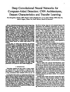
2.2.1 State Machines State machines normally use rule based architecture such as if, else and switch statements, to move the machine from one state to another depending on the conditions the machine is currently undergoing. These rule-based structures are usually broken into goals in order to keep some kind of control over the rules and give them some purpose. The goals cause the machine to change state in order to be satisfied.
Figure 2.1 – State Transition Diagram
14
Figure 2.1 shows a simple state transition that an agent might execute if an enemy is nearby. The agent has two states. If it sees an enemy it decides which state to enter depending on the status of its health. State machines are a simple technique used to implement AI in computer games; however they can suffer from large amounts of nested functions that execute the transition rules. Also as new entities are added during game development more nested functions may have to be added. These nested functions, while being time consuming and tedious to implement, are straight forward to debug, which accounts for their popularity amongst game developers. Typically state machines are used in some capacity in the majority of computer games.
2.2.2 Trigger Events A trigger is some stimulus that a game designer wants an agent to respond to such as doors, jumping pads, narrow ridges, teleporters, and sounds. Trigger events act as a level of detail control for state machines thus offering a more detailed response when a trigger is activated and so save processing power. The level of detail is controlled by hiding nested functions within a state machine until some event sets off a trigger, which reveals them thus, allowing the state machine to consider more options. Trigger events serve two main purposes in a game: (a) they keep track of events in the game world that the agents can respond to, and (b) they minimize the amount of processing that agents need to do to respond to these events. Trigger events are a useful feature in team AI, as they can be set off so as to cause the agent to look more closely at its surroundings e.g. if the agent sees a dead body on the ground it might look for blood footprints so as to shed light on where the killer might be. This would cut down on valuable processing power, as in the absence of a trigger the agent would not normally look out for such prints. When implemented well trigger events can create the illusion of a very intelligent agent to the other players in the game. Mapmakers can also place triggers within the maps directing the agent as to what to do. Examples are jumping, slowing down, ducking etc. This again reduces processing power, which would otherwise be required to evaluate what to do when the agent reaches a ledge or some other obstacle.
15
2.2.3 Intelligent Objects Getting autonomous agents to behave intelligently has plagued many a game programmer. Trying to get an AI agent to identify or locate things that let it efficiently achieve its goals is difficult. An attractive solution is to create “intelligent objects” in the virtual world of a game. This involves objects in the virtual world broadcasting what they offer to an agent that passes by. The agents do not identify these objects in the virtual world; instead they listen to what these objects are telling them. The attractiveness of the objects, in meeting the current needs of an agent, causes the agent to move towards them. Intelligent objects are one of the main AI techniques used in the highly successful computer game “The Sims” (Sims 1999). This dominated the games field when first released in 1999 due to its highly addictive game play. What made it addictive was that it was a real time interactive soap opera and a dollhouse simulator in which the AI agents appeared to act very realistically. An example of this is where a refrigerator might broadcast that it can satisfy a hunger need. Then if one of the Sims is feeling hungry and happens to walk within the influence of the refrigerator, the Sim may decide to fulfil its hunger need with that object. Another advantage, which complements the above technique, is that the programmer can use these intelligent objects to tell the agent how to interact with it. This also allows new postproduction objects to be easily added to the game thus eliminating the need to create additional animation scripts for the agent to enable it to interact with the new object. These advantages were clearly evident by the numerous expansion packs which were subsequently sold for the Sims which greatly increased the game’s longevity.
2.2.4 Fuzzy Logic Typically a computer follows Boolean logic which means that a state can have only two values either true or false. These states are usually represented as 1 or 0 respectively. Therefore if something is either true or false the AI makes a very clear cut decision which leads to very robotic and predictable responses. In real life things are not black and white and so fuzzy logic is used to resolve this issue by introducing
16
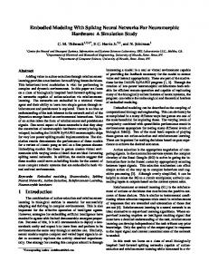
shades of grey thus allowing moderation. Fuzzy logic measures degrees of truth which is more analogous with how humans model their thoughts. In Boolean logic something either belongs to a set, or it does not. On the other hand fuzzy logic works by classifying sets that are defined by a membership function with smooth variations rather than the crisp. This membership function defines a real number (output) in the range [0,1]
Figure 2.2 – Fuzzy Logic
As Figure 2.2 shows, a membership function for Boolean logic would always return an output value of 1 or 0 no matter what the input is. Fuzzy logic however allows membership functions that can return output values between 0 and 1 depending on what input is offered. Fuzzy logic systems are particularly suited to providing smooth control and making decisions with partial truths or imprecise data. Like state machines, fuzzy systems are easy to extend incrementally. Fuzzy logic is used extensively in the game S.W.A.T 2, where it is used to model personalities for the agents’. These personalities are defined by four mental characteristics which are aggression, courage, intelligence, and cooperation respectively, therefore agents with different personalities will react differently to the same inputs. This is a simple way of giving the user the illusion of there being more intelligent agents, as agents will react in a less predictable manner.
17
2.2.5 Bayesian Networks The main concept behind Bayesian networks is their ability to reason under uncertainty. This is commonly referred to as the fog of war feature in computer games. These networks work on Bayes’ Theorem, which allows the direction of any probabilistic statement to be reversed. Bayesian networks allow modelling of the underlying causal (i.e. cause-and–effect) relationships between various phenomena and the description of this model in terms of a graph. Once a graph is constructed probability theory is used to analyse it for a variety of useful game AI tasks, such as predicting the likely outcome of a specific action, attempting to guess another player’s current situation or frame of mind, or speculation on optimal behaviour in a given situation. Bayesian networks are commonly implemented in real-time strategy games (RTS).
2.3 Learning Algorithms The ability to surprise is coupled with the ability to learn. If the player can learn to predict an AI agents’ actions and can second-guess everything that the agent does, then the agent can reasonably be said to be unintelligent. This is a common result of employing a rule-based approach. On the other hand if an agents’ behaviour is so erratic and random that it never seems to do anything sensible then we can also conclude that it is unintelligent. Therefore the general perception of intelligence is directly related to behaviour that is unpredictable, yet sensible. Implementing learning systems into games kills two birds with one stone. Firstly by creating AI Agents that constantly adapt to the players, it maintains their expectations and sustains their interest for longer periods of time. Secondly it creates a strong impression of playing in a world inhabited by intelligent agents. Until relatively recently game developers did not allocate much development time into AI for games as graphics were seen as the main selling point. Also, the lack of precedent of the successful application of learning in mainstream top-rated games means that the technology is unproven and hence perceived as high risk. Thus, most developers did not try to develop new AI techniques and instead resorted to using proven methods such as those outlined in the previous section. However learning algorithms are gradually being added to games as demonstrated by several titles that have emerged 18
onto the market such as Black & White (Lionhead 2001). This is because graphics have become a commodity item and so is no longer a differentiating factor. Pattern Recognition One of the simplest learning techniques being implemented in games today is pattern recognition (Mommersteeg-Eindhoven 2002). Here repetitive player events are monitored by the AI agent, who in turn tries to decipher a pattern that it can then use to predict what the player is doing or going to do. These algorithms are relatively easy to implement and can produce very realistic behaviour on behalf of the agent. Case-based reasoning Case-based reasoning (CBR) (Leake 1996) is the process of solving new problems based on the solutions to similar past problems. If a problem has been encountered before, the system retrieves the appropriate solution, otherwise it will try and solve the problem based on the knowledge it has for similar problems and then save the solution for future reference. At the highest level of generality a CBR cycle, for when the exact problem is not found, may be described by the following four processes: 1. RETRIEVE the most similar case or cases 2. REUSE the information and knowledge in that case to solve the problem 3. REVISE the proposed solution 4. RETAIN the parts of this experience likely to be useful for future problem solving Essentially CBR is like a database full of solutions to various problems and if it encounters a problem it does not have a solution to it creates a solution based on the knowledge it has therefore, has the ability to learn to solve new problems. A problem with CBR is that it often requires large amounts of memory for storing the database. Decision Trees A decision tree (Mitchell 1997) is a graph of decisions and their possible consequences, including resource costs and risks, used to create a plan to reach a goal. 19
Decision trees are constructed in order to help with making decisions. They make a decision based on a set of inputs starting at the root, and at each node, selecting a child node based on the value of one input. Decision tree learning is a method for approximating different target functions, in which the learned function is represented by a decision tree. Learned trees can also be re-represented as sets of if-then rules to improve human readability. Typically, decision trees are constructed using an induction algorithm, such as ID3 (Quinlan 1986), which constructs a tree based on the classification of a training set of data. The main draw back from the learning algorithms mentioned above is that they rely on learning from a training set which has an expected output for each input in the set, but what if the output is unknown? Two forms of learning algorithms that can learn without knowing the correct output for each input are neural networks and genetic algorithms. In the next sections these will be discussed in detail.
2.4 Neural Networks Neural Networks (NNs) are a class of machine learning techniques based on the neural interconnections in biological brains and nervous systems. Artificial neural networks operate by repeatedly adjusting the internal numeric parameters (or weights) between interconnected components of the network, allowing them to learn a near optimal response for a wide variety of different classes of learning tasks. Neural networks are used in the game Black & White (Lionhead 2001) where the player has to teach a creature in the game what to do. The creature is taught using the “slap and tickle” approach to adjust the weights in the neural network (Barnes and Hutchens 2002). The successful use of NN in this game is likely to encourage more developers to investigate its use. An artificial neural network is an information-processing system that has certain performance characteristics in common with biological neural networks (Fausett 1994). Artificial Neural networks have been developed as generalizations of mathematical models of human cognition or neural biology, based on the following assumptions: 1. Information processing occurs in simple elements called neurons
20
2. Signals are passed between neurons over connection links 3. Each of these connections has an associated weight which alters the signal 4. Each neuron has an activation function to determine its output signal. An artificial neural network is characterised by (a) the pattern of connections between neurons i.e. the architecture, (b) the method of determining the weights on the connections (Training and Learning algorithm), and (c) the activation function.
Figure 2.3 – Pattern Recognition Training Set
An everyday example of how NN are used is in character recognition. Taking the example shown in figure 2.3 the NN is able to decipher from 8x8 grids what character is being displayed. Therefore the NN has 64 inputs (one for each square in the grid) and depending on the state of each square, either 0 or 1, the NN can learn to associate them with a character.
2.4.1 The Biological Neuron A biological neuron has three types of components that are of particular interest in designing an artificial neuron: dendrites, soma, and axon, all of which are shown in Figure 2.4. 21
Figure 2.4 – Biological Neuron
•
Dendrites receive signals from other neurons (synapses). These signals are electric impulses that are transmitted across a synaptic gap by means of a chemical process. This chemical process modifies the incoming signal.
•
Soma is the cell body. Its main function is to sum the incoming signals that it receives from the many dendrites connected to it. When sufficient input is received the cell fires sending a signal up the axon.
•
The Axon propagates the signal, if the cell fires, to the many synapses that are connected to the dendrites of other neurons.
2.4.2 The Artificial Neuron
Figure 2.5 – Artificial Neuron
22
An artificial neuron is an attempt to mimic, in software, the behaviour of the biological neuron. The artificial neuron structure is composed of (i) n inputs, where n is a real number, (ii) an activation function and (iii) an output. Each one of the inputs has a weight value associated with it and it is these weight values that determine the overall activity of the neural network. Thus when the inputs enter the neuron, their values are multiplied by their respective weights. Then the activation function sums all these weight-adjusted inputs to give an activation value (usually a floating point number). If this value is above a certain threshold the neuron outputs this value, otherwise the neuron outputs a zero value. The neurons that receive inputs from or give outputs to an external source are called input and output neurons respectively. Thus the artificial neuron resembles the biological neuron in that (i) the inputs represent the dendrites and the weights represent the chemical process that occurs when transferring the signal across the synaptic gap, (ii) the activation function represents the soma and (iii) the output represents the axon.
2.4.3 Layers It is often convenient to visualise neurons as arranged in layers with the neurons in the same layer behaving in the same manner. The key factor determining the behaviour of a neuron is its activation function. Within each layer all the neurons typically have the same activation function and the same pattern of connections to other neurons. Typically there are three categories of layers, which are Input Layer, Hidden Layer and Output Layer respectively. Input Layer Neurons in the input layer do not have neurons attached to their inputs. Instead these neurons have only one input from an external source. Also the inputs are not weighted and so are not acted upon by the activation function. Each neuron receives one input from an external source and passes this value directly to the nodes in the next layer. Hidden Layer The neurons in the hidden layer receive inputs from the neurons in the previous input/hidden layer. These inputs are multiplied by their respective weights, summed
23
together, and then presented to the activation function which decides if the neuron should fire or not. There can be many hidden layers present in a neural network although for most problems one hidden layer is sufficient. Output Layer The neurons in the output layer are similar to the neurons in a hidden layer except that their outputs do not act as inputs to other neurons. Their outputs however represent the output of the entire network.
2.4.4 Activation Function The same activation function is typically used by all the neurons in any particular layer of the network. However this condition is not required. In multi-layer neural networks the activation used is usually non-linear, in comparison with the step or binary activation functions used in single layer networks. This is because feeding a signal through two or more layers using linear functions is the same as feeding it through one layer. The two functions that are mainly used in neural networks are the Step function and the Sigmoid function (S-shaped curves) which represent linear and non-linear functions respectively. Figure 2.6 shows the three most common activation functions, which are binary step, binary sigmoid, and bipolar sigmoid functions respectively.
Figure 2.6 – Activation Functions
24
2.4.5 Learning The weights associated with the inputs to each neuron are the primary means of storage for neural networks. Learning takes place by changing these weights. There are many different techniques that allow neural networks to learn by changing their weights. These broadly fall into two main categories, which are supervised learning and unsupervised learning respectively. Supervised Learning The techniques in the supervised category involve mapping a given set of inputs to a specified set of target outputs. This means that for every input pattern presented to the network the corresponding expected output pattern must be known. The main approach in this category is backpropagation, which relies on error signals from the output nodes. This requires guidance from an external source i.e. a supervisor to monitor the learning through feedback. Training a neural network by backpropagation involves three stages: the feed forward of the input training pattern, the backpropagation of the associated output error, and the adjustments of the weights to minimise this error. The associated output error is calculated by subtracting the networks output pattern from the expected pattern for that input training pattern. Unsupervised Learning The techniques that fall into the unsupervised learning category have no knowledge of the correct outputs. Therefore, only a sequence of input vectors is provided. However the appropriate output vector for each input is unknown. Reinforcement learning is an example of an unsupervised approach. In reinforcement learning the feedback is simply a scalar value, which may be delayed in time. This reinforcement signal reflects the success or failure of the entire system after it has preformed some sequence of actions. Hence the reinforcementlearning signal does not assign credit or blame to any one action. This method of learning is often referred to as the “Slap and Tickle approach” (Barnes and Hutchens
25
2002). Reinforcement learning techniques are appropriate when the system is required to learn on-line, or a teacher is not available to furnish error signals or target outputs.
2.4.6 Training There are two main properties associated with training a NN which are generalization and overfitting. These will now be explained in more detail. Generalization
Figure 2.7 – Generalization
When the learning procedure is carried correctly, the network will be able to generalise. This means that it will be able to handle scenarios that it did not encounter during the training process. This is due to the way the knowledge is internalised by the network. Since the internal representation is neuro-fuzzy, practically no cases will be handled perfectly and so there will be small errors in the values outputted. However it is these small errors that enable the network to handle different situations in that it will be able to abstract what it has learned and apply it to these new 26
situations. In this way it can handle scenarios that it did not encounter during the training process. This is known as generalisation. For example, suppose a NN is trained for character recognition with the training set in figure 2.7. If the training is done correctly and the NN is presented with the test cases in figure 2.7, which differ slightly from anything in the training set, it should be able to generalise, from what it has learned, and give the correct output. The opposite of generalisation is overfitting. Overfitting
Figure 2.8 - Overfitting
Overfitting describes when a NN has adapted its behaviour to a specific set of states but performs badly when presented with states that differ slightly and therefore has lost its ability to generalise. This situation arises when the NN is over trained i.e. the learning is halted only when the NN’s output exactly matches the expected output.
2.4.7 Topology The topology of a NN refers to the layout of its nodes and how they are connected. There are many different topologies for a fixed neuron count, but most structures are either obsolete or practically useless. The following are examples of well-documented topologies that are best suited for game AI. Feed forward This is where the information flows directly from the input to the outputs. Evolution and training with back propagation are both possibilities. There is a connection restriction as the information can only flow forwards hence the name feed forward. 27
Recurrent These networks have no restrictions and so the information can flow backward thus allowing feedback. This provides the network with a sense of state due to the internal variables needed for the simulation. The training process is however more complex than the feed forward because the information is flowing both ways. Genetic algorithms (GA) (Russel and Norvig 1995) can be used to evolve the weights of a NN of any topology and is suitable for supervised and unsupervised learning. They also provide a straightforward method of producing a NN which can generalise. Genetic algorithms will be outlined in detail in the following sections. GAs are a powerful and flexible method of training a NN of any topology. They also have the benefit of being able to perform supervised and unsupervised training and provide useful strategies to produce NNs that can generalise.
2.5 Genetic Algorithms It transpires that what is good for nature is also good for artificial systems, especially if the artificial system includes a lot of non-linear elements. The genetic algorithm, described in (Russel and Norvig 1995), works by filling a system with organisms each with randomly selected genes that control how the organism behaves in the system. Then a fitness function is applied to each organism to find the two fittest organisms for this system. These two organisms then each contribute some of their genes to a new organism, their offspring, which is then added to the population. The fitness function depends on the problem, but in any case, it is a function that takes an individual as an input and returns a real number as an output. The genetic algorithm technique attempts to imitate the process of evolution directly, performing selection and interbreeding with randomised crossover and mutation operations on populations of programs, algorithms, or sets of parameters. Genetic algorithms and genetic programming have achieved some truly remarkable results in recent years, effectively disproving the public misconception that a computer “can only do what we program it to do”.
28
Once a fitness score has been assigned to each individual organism in the population there are three more important aspects of the genetic algorithm which are selection, crossover, and mutation. Each of these will now be explained in more detail.
2.5.1 Selection The selection process involves selecting two or more organisms to pass on their genes to the next generation. There are many different methods used for selection. These range from randomly picking two organisms with no weight on their fitness score to sorting the organisms based on their fitness scores and then picking the top two as the parents. The main selection methods used by the majority of genetic algorithms are: Roulette Wheel selection, Tournament selection, and Steady State selection. Another important factor in the selection process is how the fitness of each organism is interpreted. If the fitness is not adjusted in any way it is referred to as the raw fitness value of the organism, otherwise it is called the adjusted fitness value. The reason for adjusting the fitness values of the organisms is to give them a better chance of being selected when there are large deviations in the fitness values of the entire population. Tournament Selection In tournament selection, n organisms are selected at random and the fittest of these organisms is chosen to add to the next generation. This process is repeated as many times as is required to create a new population of organisms. The selected organisms are not removed from the population and so can be chosen any number of times. This selection method is very efficient to implement as it does not require any adjustment to the fitness value of each organism. The drawback with this method is that it can get stuck in local minima because it can converge quickly on a solution that may not be the best one. Roulette Wheel Selection Roulette wheel selection is a method of choosing organisms from the population in a way that is proportional to their fitness value. This means that the fitter the organism, the higher the probability it has of being selected. This method does not guarantee that the fittest organisms will be selected, merely that they have a high probability of
29
being selected. It is called roulette wheel selection because the implementation of it involves representing the populations total fitness score as a pie chart or roulette wheel. Each organism is assigned a slice of the wheel where the size of each slice is proportional to that respective organism’s fitness value. Therefore the fitter the organism the bigger the slice of the wheel it will be allocated. The organism is then selected by spinning the roulette wheel as in the game of roulette. This roulette selection method is not as efficient as the tournament selection method because there is an adjustment to each organism’s fitness value in order to represent it as a slice in the wheel. Another drawback with this approach is that it is possible that the fittest organism will not get selected for the next generation. However this method benefits from not getting stuck in as many local minima. Steady State Selection Steady state selection always selects the fittest organism in the population. This method retains all but a few of the worst performers from the current population. This is a form of elitism selection as only the fittest organisms have a chance of being selected. This method usually converges quickly on a solution but often this is just a local minima of the complete solution as shown in Figure 2.9.
Figure 2.9 – Global Minima
The main drawback with this method is that it tends to always select the same parents every generation, which results in a dramatic reduction in the gene pool used to create the child. This is why the population tends to get stuck in local minima as it is over relying on mutation to create a better organism. This method is ideal for tackling 30
problems that have no local minima or for initially getting the population to converge on a solution in conjunction with one of the other selection methods.
2.5.2 Crossover The crossover process is where a mixture of the parent’s genes is passed onto the new child organism. There are three main approaches to this random crossover, singlepoint crossover and two-point crossover. Random Crossover For each of the genes in the offspring’s chromosome a random number of either zero or one is generated. If the number is zero the offspring will inherit the same gene in Parent 1 otherwise the offspring will inherit the appropriate gene from Parent 2. This results in the offspring inheriting a random distribution of genes from both parents.
Figure 2.10 –Random Crossover
Single-Point Crossover A random crossover point is generated in the range (0 < Pt 1 < length of Offspring chromosome). The offspring inherits all the genes that occur before Pt1 from Parent 1 and all the genes that occur after Pt1 from Parent 2.
31
Figure 2.11 Single-point crossover
Two-Point Crossover This is the same as the single-point crossover except this time two random crossover points are generated. The offspring inherits all the genes before Pt1 and after Pt2 from Parent 1 while all the genes between Pt1 and Pt2 are inherited from Parent 2.
Figure 2.12 Two-point Crossover
2.5.3 Mutation Mutation is used in conjunction with the crossover phase in genetic algorithms as it results in the creation of new genes that are added to the population. This technique is used to enable the genetic algorithm to get out of local minima. The mutation is controlled by the mutation rate of the genetic algorithm and is the probability that a gene in the offspring will be mutated. Mutation occurs during the crossover stage; when the child is inheriting its genes form the parent organisms each gene is checked against the probability of a mutation. If this condition is met then that gene is mutated.
32
Although this usually means a quick death for the mutated individual, some mutations lead to a new successful species.
2.6 Potential Problems There is general belief among developers and game companies that quality assurance would prove difficult if not impossible if the AI agents started behaving in unpredictable and continually evolving ways. This is currently perceived to be the major barrier to the use of advanced AI because of the potential maintenance difficulties that might ensue. An example of this is when the game is shipped the developer has no control over any of the modified algorithms, many of which could make the game worse. As a consequence this why most developers do not even consider investigating the use of more sophisticated AI. Neural networks and genetic algorithms are also difficult to apply in games due to their relatively low efficiency. The following are some of the problems commonly encountered when constructing a Learning AI: •
Mimicking Stupidity – When teaching an AI by copying a human players strategy you may find that the computer is taught badly
•
Overfitting – When an AI has learnt from its experience of encountering problems in one level it may try this learning when attempting a new level. For example, if the AI had found that when opening doors it has to escape the line of fire by diving behind a wall to its left, it will assume this as a generalised tactic and apply it unthinking in another level. This could lead to amusing behavioural defects if not corrected
•
Set Behaviour – Once an agent has a record of its past behaviours, does it stick to the behaviour which has been most successful, or does it try new methods in an attempt to improve?
2.7 Conclusions This chapter looked at the use of AI in the Computer Games industry and suggested that the main barrier to its more sophisticated use is the drain it puts on CPU resources 33
at the expense of graphics. However, with graphics being increasingly put onto dedicated boards and becoming a commodity in the majority of games, this conflict is rapidly diminishing. Another obstacle is the general belief that quality assurance would prove impossible if the AI agents started behaving in unpredictable and continually evolving ways. This is currently perceived to be the major barrier to the use of advanced AI because of the potential maintenance difficulties that might ensue, and is the main reason why most developers do not consider investigating it. Most computer game AI is rule-based and this has resulted in predictable AI agents which, once noticed by the player, erode away at their immersive experience within the virtual world. Learning algorithms offer richer possibilities and allow the potential of solving problems that cannot be solved with other methods. One such problem is that of pathfinding in dynamic environments. In the next chapter we will discuss this problem in detail and then move on to show how it can be solved using the AI learning techniques just outlined.
34
Chapter 3 Pathfinding In this chapter we discuss the pathfinding problem in computer games. We describe current approaches to solving it and then propose that the AI learning techniques detailed in the previous chapter provide an ideal way of tackling it.
3.1 Background One of the greatest challenges in the design of realistic Artificial Intelligence (AI) in computer games is agent movement. Pathfinding strategies are usually employed as the core of any AI movement system. This chapter will highlight the various pathfinding algorithms presently used in computer games and discuss their shortcomings, especially when dealing with real-time pathfinding. In addition a variety of algorithms, used in other fields such as robotics, will be discussed in relation to their applicability in computer games. Perhaps the main drawback of traditional pathfinding AI is that it only works efficiently in static game environments. Thus with real-time physics engines now coming as standard in most new games this static limitation is hindering the full potential of the games. A game physics engine allows objects within the game word to interact with each other by simulating the laws of physics, such as gravity. This allows the introduction of unscripted dynamic objects to the game world which the player and any other dynamic objects can interact with. It creates a much more immersive experience for the player but is rarely utilised to its full potential. This is because the number of dynamic objects within the game has to be limited due to traditional pathfinding algorithms’ dependence on a static environment. This suggests that there is a need for real-time pathfinding techniques to complement and enhance current computer games. Typically the world geometry in a game is stored in a structure called a map. Maps contain all the polygons that make up the game environment. Writing code to get an AI agent to navigate through a game map is a complex problem. While it is 35
mathematically possible to calculate paths around the geometry in the map it can be computationally expensive. To overcome this most game developers use precomputed pathfinding data that is invisible to the player. This allows the agent to easily navigate the map. This precomputed data is typically a simplified representation of the map structure. There are three main steps to pathfinding in computer games, namely (1) preprocessing the game map (2) creating a graph with this data and (3) using a search algorithm to transverse (search) the graph for a solution. These three steps will now be explained in more detail.
3.2 Pre-processing Game Worlds The general methodology used to cut down the search space of the virtual world for the pathfinder is to divide up the world’s geometry into smaller sections. The pathfinder then uses this simplified representation of the world to determine the best path from the starting point to the desired destination in the world. The most common forms of simplified representations used are (1) Binary Space Partition trees, (2) Waypoints, (3) Navigation Meshes, (4) Area Awareness System
3.2.1 Binary Space Partition trees (BSP) BSP trees (Fuchs, Kedem et al. 1980) are usually applied to world geometry as a type of spatial sorting. Since the computation involved is generally too expensive to perform at runtime the spatial sorting is done on static world geometry. A BSP tree for a group of objects is constructed by dividing and sorting the world’s geometry into two groups: objects lying on the positive side of the plane and those located on the negative side of the plane (Lengyel 2002). Each node in the tree represents a convex subspace and stores a plane, which splits the space the node represents into two halves. A node also stores references to two other (child) nodes, which represent each half. Each half-space is partitioned by a recursive application of the method until some final condition is met. Traditionally the partitioning planes of a BSP tree have been aligned to the polygons that make up the world geometry (Akenine-Moller and Haines 2002). However BSP trees represent only a static representation of the virtual
36
world and so it is incapable of handling any dynamic changes that could occur. On the plus side BSP trees can also be used by other elements of a game engine to achieve: •
Real time generation of shadows
•
Intelligent camera planning
•
Fast collision detection
3.2.2 Waypoints The waypoint system (Sterren 2001) for navigation is a collection of nodes (points of visibility) with links between them. Travelling from one waypoint to another is a sub problem with a simple solution. All places reachable from waypoints should be reachable from any waypoint by travelling along one or more other waypoints, thus creating a grid or paths that the AI agent can walk on. If an AI agent wants to get from A to B it walks to the closest waypoint seen from position A, then uses a precalculated route to walk to the waypoint closest to position B and then tries to find its path from there. Usually the designer manually places these waypoint nodes in a map to get the most efficient representation. This system has the benefit of representing the map with the least amount of nodes for the pathfinder to deal with. However it still has the weakness in that it cannot cope with dynamic changes as the waypoints represent a static obstacle free map. Another limitation occurs when the agent is not at a waypoint and as such it has to search for the nearest unobstructed waypoint, which can be a computational expensive action. Figure 3.1 shows how a simple scene would be represented with waypoints and the corresponding Table 3.1 shows the routing information contained within each waypoint. The path from (A) to (B) is executed as follows. A straight-line path from (A) to the nearest waypoint is calculated (P1), then a straight-line path from (B) to the nearest waypoint is calculated (P2). Looking at the linking information, a pathfinding system will find a path between 6 and 3 as follows: { P1, waypoint 6, waypoint 5, waypoint 2, waypoint 3, P2 }.
37
Figure 3.1 – Waypoint System
Way Point Number
Link Information
1
4
2
3, 5
3
2
4
1, 5
5
2, 4
6
5
Table 3.1
3.2.3 Navigation Meshes A navigation mesh is a set of convex polygons that describe the “walkable” surface of a 3D environment as shown in Figure 3.2 (Board and Ducker 2002). Algorithms are then used abstract the information from map structures to generate a Navigation Mesh for that map. This navigation mesh is composed of convex 2D polygons which when assembled together represent the shape of the map like a floor plan. The polygons in the mesh must be convex since this guarantees that the AI agent can move in a single straight line from any point in one polygon to the centre point of any adjacent polygon (White and Christensen 2002). Each of the convex 2D polygons is used as a node for a pathfinding algorithm. A navigation mesh path consists of a list of adjacent nodes to
38
travel on. Convexity guarantees that with a valid path the AI agent can simply walk in a straight line from one node to the next on the list. While computationally more complex to create, they overcome the problem encountered by waypoints when the agent is not near a waypoint. This is due to the fact that the agent will always reside within one of the convex 2D polygons in the mesh and so no expensive tracing is required. However a navigational mesh still has the limitation that it cannot cope with dynamic changes as it also represents a static representation of a game map.
Figure 3.2 – Navigation Mesh
3.2.4 Area Awareness System (AAS) J.P van Waveren designed this system for his gladiator Quake II bot (AI agent) as part of his master’s thesis (Waveren 2001). This system was adopted and extended by Id Software for their Quake III Arena game. In essence a pre-processing phase extracts adjacency information form Id’s proprietary BSP structure. This builds a static representation of the world geometry in the form of 3D convex polygons, which is tweaked for dynamic conditions such as the opening of doors. Given any point in the space, the system can find which area it is in, and determine a path to any other point using “hierarchal routing”, as the author refers to it. The 3D convex polygons that represent an area such as a room are grouped together into a structure called a cluster. A map is usually composed of a number of clusters connected by portals i.e. the portals would represent the areas or hallways connecting 39
two or more rooms. The hierarchal routing then works by finding a path from within a cluster to the portal nearest to the goal and at the same time finds which portals will need to be travelled through to get to the goal. The main difference between AAS and navigation meshes is that the AAS system provides reachability triggers on the boundaries of each area and each area is represented by a 3D convex polygon whereas the navigational meshes do not. These triggers, referred to as reachabilities, tell the bot how it can reach the next area and are calculated for each area that links to another area. The different types of reachabilities used in Quake III Arena are listed below: •
Swimming in a straight line
•
Walking in a straight line
•
Crouching in a straight line
•
Jumping onto a barrier
•
Jumping out of water
•
Jumping
•
Teleporting
•
Using an elevator
•
Using a jump pad
•
Using a moving platform
•
Rocket jumping
These triggers are a simple way of giving the AI agent the appearance of intelligence. In reality its reactions are basically scripted once it encounters one e.g. jumping from one platform to another. Once again the limitations of this approach become apparent when dynamic objects are added to the scene.
40
3.3 Searching Graphs Pathfinding algorithms can be used once the geometry of a game world has been encoded as a map and pre-processed to produce one of the structures discussed in section 3.2 such as a navigation mesh or a set of waypoints. Since the 2D polygons in the navigation mesh and the points in the waypoint system are all connected in some way, they constitute vertices or nodes in a graph. All the pathfinding algorithm has to do is tranverse the graph until it finds the endpoint it is looking for. Conceptually, a graph G is composed of two sets, and can be written as G = (V,E) where: •
V – Vertices: A set of discreet points in n-space, in our case this corresponds to a 3D map.
•
E – Edges: A set of connections between the vertices which can have costs associated with them such as the distance between the two vertices.
In addition to this structural definition, pathfinding algorithms generally need to know about the properties of these elements. For example, the length, travel-time, or general cost of every edge needs to be known. (From this point on cost will refer to the distance between two nodes).
3.4 Traditional Algorithms In many game designs AI is about moving agents around in a virtual world. It is useless to develop complex systems for “high-level decision making” if an agent cannot find its way around a set of obstacles to implement that decision. On the other hand if an AI agent can understand how to move around the obstacles in the virtual world even simple decision-making structures can look impressive. Thus the pathfinding system has the responsibility of understanding the possibilities for movement within the virtual world. A pathfinder will define a path through a virtual world to solve a given set of constraints. An example of a set of constraints is to find the shortest path to take an agent from its current position to the target position. Pathfinding systems typically use the pre-processed representations of the virtual world as their search space.
41
There are many different approaches to pathfinding algorithms. At a high level they can be divided into two main categories, undirected and directed pathfinding respectively. Within the bounds of these two categories the main concepts for each will be discussed.
3.4.1 Undirected This approach is analogous to a rat in a maze running around blindly trying to find a way out. The rat spends no time planning a way out and puts all its energy into moving around. Thus the rat might never find a way out and so uses most of the time going down dead ends. A design based completely on this concept would not be useful in creating a believable response for an AI agent. It does however prove useful in getting an agent to move quickly, while in the background a more sophisticated algorithm finds a better path. There are two main undirected approaches that improve efficiency. These are Breadth-first search and Depth-first search respectively (Russel and Norvig 1995). Breadth-first search treats the virtual world as a large connected graph of nodes. It will expand all nodes that are connected to the present node and then in turn expand all the nodes connected to these new nodes. Therefore if there is a path the breadthfirst approach will find it. In addition if there are several paths it will return the shallowest solution first. The depth-first approach is the opposite of breadth-first searching in that it looks at all the children of each node before it looks at the rest, thus creating a linear path to the goal. Only when the search hits a dead end does it go back and expand nodes at shallower levels. For problems that have many solutions the depth-first method is usually better as it has a good chance of finding a solution after exploring only a small portion of the search space. For clarity the two approaches will be explained using the simple map shown in Figures 3.3 and 3.4.
42
Figure 3.3 – Simple map with search tree
Figure 3.3 shows a waypoint representation of a simple map and its corresponding complete search tree from the start (S) to the goal (G).
Figure 3.4 – Breadth-First and Depth-First Search
Figure 3.4 shows how the two approaches would search the tree to find a path. In this example the breadth-first took four iterations while the depth-first search finds a path in two. This is because the problem has many solutions, which the depth-first approach is best suited to. The main drawback in these two approaches is that they do not consider the cost of the path, but they are effective if no cost variables involved.
3.4.2 Directed The different designs in this category all have one thing in common in that they do not go blindly through the maze. In other words they all have some method of assessing their progress from all the adjacent nodes before picking one of them. This is referred
43
to as assessing the cost of getting to the adjacent node. Most of the algorithms used will find a solution to the problem but not always the most efficient solution i.e. the shortest path. The main strategies for directed pathfinding algorithms are: •
Uniform cost search g(n) modifies the search to always choose the lowest cost next node. This minimises the cost of the path so far. It is optimal and complete, but can be very inefficient.
•
Heuristic search h(n) estimates the cost from the next node to the goal. This cuts the search cost considerably, but it is neither optimal nor complete.
The two most commonly employed algorithms for directed pathfinding in games use one or more of the above strategies. These directed algorithms are known as Dijkstra and A* respectively (Dijkstra 1959; Russel and Norvig 1995). The Dijkstra algorithm uses the uniform cost strategy to find the optimal path, while the A* combines both strategies thereby minimizing the total path cost. Thus A* returns an optimal path and is generally much more efficient than Dijkstra making it the backbone behind almost all pathfinding designs in computer games. Since A* is the most commonly used algorithm in the pathfinding arena it will be outlined in more detail later in this chapter. The following example in Figure 3.5 compares the effectiveness of Dijkstra with A*. This uses the same map from Figure 3.3 and its corresponding search tree from start (S) to the goal (G). However it also includes the costs of getting from one node to another.
Figure 3.5 – Simple map with path costs
44
Figure 3.6 – Dijkstra and A* Search
Figure 3.6 illustrates how the two algorithms would search the tree to find a path given the costs indicated in Figure 3.5. In this example Dijkstra took three iterations while A* search finds a path in two to find the shortest path i.e. the optimal solution. Given that the first stage shown in Figure 3.6 for both Dijkstra and A* actually represents three iterations, as each node connected to the start node (S) would take one iteration to expand, the total iterations for Dijkstra and A* are six and five respectively. When compared to Breadth-first and Depth-first algorithms, which took five and two iterations respectively to find a path, they took more iterations but they both returned optimal paths while breadth-first and depth-first did not. Generally unless an AI agent in a virtual world follows an optimal path the user perceives it as a lack of intelligence. Many directed pathfinding designs use a feature known as Quick Paths (Higgins 2002). This is an undirected algorithm that gets the agent moving while in the background a more complicated directed pathfinder assesses the optimal path to the destination. Once the optimal path is found a “slice path” is computed which connects the quick path to the full optimal path. This creates the illusion that the agent computed the full path from the start.
3.5 A* Pathfinding Algorithm A* (pronounced A-star) is a directed algorithm (Hart, Nilsson et al. 1968), meaning that it does not blindly search for a path (unlike a rat in a maze) (Matthews 2002).
45
Instead it assesses the best direction to explore, sometimes backtracking to try alternatives means. This means that A* will not only find a path between two points (if one exists!) but it will find the shortest path, and do so relatively quickly.
3.5.1 Implementation The map has to be prepared or pre-processed before the A* algorithm can work. This involves breaking the map into different points or locations, which are called nodes. These can be waypoints, the 2D polygons of a navigation mesh or the polygons of an area awareness system. These nodes are for recording the progress of the search. In addition to storing the map location each node has three other attributes that help guide the algorithm from a start node to the goal node. These are the uniform, heuristic, and the total path fitness costs, commonly known as g, h, and f respectively. Different values can also be assigned to paths between the nodes. Typically these would be the distances between the nodes. The attributes g, h, and f are defined as follows: •
g is the cost of getting from the start node to the current node i.e. the sum of all the values in the path between the start and the current node
•
h stands for heuristic which is an estimated cost from the current node to goal (usually the straight line distance from this node to the goal)
•
f is the sum of g and h and is the best estimate of the cost of the path going through the current node. In essence the lower the value of f the more efficient the path
The purpose of g, h, and f is to quantify how promising a path is up to the present node. Additionally A* maintains two lists, an Open and a Closed list. The Open list contains all the nodes in the map that have not been fully explored yet, whereas the Closed list consists of all the nodes that have been fully explored. A node is considered fully explored when the algorithm has evaluated every node linked to it. Nodes therefore simply mark the state and progress of the search. Another important attribute assigned to each node is a reference to its parent node. When a node (N) is being fully explored by the algorithm every node linked to N (child nodes) will have N as their parent node. Once the goal is found the algorithm uses the parent node 46
attribute from the nodes in the closed list to backtrack from the goal node to the start node. The pseudo-code for the A* Algorithm is as follows: 1. Let S = Start Node. 2. Assign g, h and f values to S. a. Parent Node for S = NULL b. Put S on Open List 3. Let B = the best node from the Open List (i.e. the node that has the lowest f-value). a. If Open List is Empty (i)
Return “Path cannot be found”
b. Else If B is the Goal Node (i)
Put B on Closed List
(ii)
GOTO Step 6
c. Else Put B on Closed List 4. For All Child Nodes connected to B a. Let C = Child Node. b. If C NOT on Open List AND C NOT on Closed List (i) Assign g, h, and f values to C. (ii) Parent Node for C = B (ii) Put C on Open List 5. Repeat from Step 3 6. Let P = Path 7. Let N = Last Node on Closed List 8. Add N to Path a. N = Parent Node for N b. If N = Start Node (i) Return Path c. Else, Repeat from Step 8
The following step through example should help clarify how the A* algorithm works (see Figure 3.7). 47
Figure 3.7 – A* Example
Let the centre (1,4) node be the starting point (S), and the offset grey node (1,1) the goal position (G). The h-value is calculated differently depending on the application. However for this example h will be the combined cost of the vertical and horizontal distances from the present node to (G). Therefore h = | gx-cx | + | gy-cy | where (gx,gy) is the goal node and (cx,cy) is the current node. At the start since S(1,4) is the only node that the algorithm knows it places it in the Open list as shown in Table 3.1. This is steps 1 and 2 from pseudo code. The affix P[…] denotes the parent node attribute for each node. Since the start node has no parent node it is assigned to NULL which means none. Open List { S(1,4)P[NULL]; }
Closed List { Empty }
Table 3.2 Step 3 requires that the node with the lowest f-value in the open list be selected. Since S(1,4) is the only node in the open list currently it is selected. Since it is not the goal node it is placed on the closed list and step 4 is implemented.
48
There are two neighbouring (child) nodes to S(1,4). These are (1,3) and (1,5) respectively. Since neither of these nodes is already in the Open list they are added to it with their parent node attribute set to S(1,4). Then each node in the Open list is checked to see if it is the goal node G(1,0) and if not then its f- value is calculated as outlined in steps 4b(i – iii). g-value
Node (1,3)
0 (Nodes to travel through)
(1,5)
h-value
f-value
|1-1| + |1-3| = 2
2
4
4
0 Table 3.3
As can be seen from Table 3.3 Node (1,3) has the lowest f-value and is therefore the next node to be selected by the A* algorithm. Since all the neighbouring nodes to S(1,4) have been looked at S(1,4) is added to the Closed list (as shown in Table 3.3) and step 3 is repeated. Open List
Closed List
{ S(1,4)P[NULL]; }
{ Empty }
{ (1,3)p[S] ; (1,5)p[S] }
{ S(1,4)P[NULL]; } Table 3.4
This time node (1,3) is selected as the best node as it has the lowest f-value. There are no neighbouring nodes to (1,3) that are not already in the open or closed lists. Therefore (1,3) gets added to the closed list and step 3 is repeated. Since (1,5) is the only node in the open list, and thus has the lowest f-value, it is now looked at. (1,6) is the only child node of (1,5) that is not in either the closed or open list and is therefore added to the open list with the appropriate g, h, f values, and with (1,5) as its parent node.
49
Open List
Closed List
{ S(1,4)p[NULL] }
{ Empty }
{ (1,3)p[S] ; (1,5)p[S] }
{ S(1,4)P[NULL]; }
{ (1,5)p[S] }
{ S(1,4)p[NULL] ; (1,3)p[S] }
{ (1,6)p[1,5] }
{ S(1,4)p[NULL] ; (1,3)p[S] ; (1,5)p[S] } Table 3.5
This is repeated until step 3 finds one of the child nodes to be the goal node G(1,1). For the complete table with all the open and closed list values for this example see Appendix A. Once the goal node is found it is added to the closed list and the algorithm moves to step 5. Closed List { S(1,4)p[NULL] ; (1,3)p[S] ; (1,5)p[S] ; (1,6)p[1,5] ; (2,6)p[1,6] (3,4)p[3,5] ; (3,3)p[3,4] ; (4,6)p[3,6] ; (5,6)p[4,6] ; (5,5)p[5,6] ;
; (3,6)p[2,6] ; (3,5)p[3,6] ; (5,4)p[5,5] ; (5,3)p[5,4] ;
(5,2)p[5,4] ; (5,1)p[5,2] ; (4,1)p[5,1] ; (3,1)p[4,1] ; (2,1)p[3,1] ; G(1,1)p[2,1] } Table 3.6 Table 3.6 contains all the nodes in the closed list as the algorithm enters step 5. Therefore the last node G(1,1) becomes N and gets added to the path. Then N moves to the node assigned to its parent node i.e. (2,1). This is repeated until the start node has been reached. Path = { G(1,1), (2,1), (3,1), (4,1), (5,1), (5,2), (5,3), (5,4), (5,5), (5,6), (4,6), (3,6), (2,6), (1,6), (1,5), S(1,4) } This algorithm will always find the shortest path if one exists [Matthews02].
3.5.2 Limitations of A* A* requires a large amount of CPU resources if there are many nodes to search through as is the case in large maps which are becoming popular in the newer games. 50
In sequential programs this may cause a slight delay in the game. This delay is compounded if A* is searching for paths for multiple AI agents and/or when the agent has to move from one side of the map to the other. This drain on CPU resources may cause the game to freeze until the optimal path is found. Game designers overcome these problems by tweaking the game so as to avoid these situations (Cain 2002). The inclusion and/or introduction of dynamic objects to the map is also a major problem when using A*. For example once a path has been calculated, if a dynamic object then blocks the path the agent would have no knowledge of this, and would continue on as normal and walk straight into the object. Simply reapplying the A* algorithm every time a node is blocked would cause excessive drain on the CPU. There has been research into extending the A* algorithm to deal with this problem most notably the D* algorithm (which is short for dynamic A*) (Stentz 1994). This allows for the fact that node costs may change as the AI agent moves across the map and presents an approach for modifying the cost estimates in real time. However the drawback to this approach is that it adds further to the drain on the CPU and so forces a limit on the number of dynamic objects than can be introduced to the game. A key issue constraining the advancement of the games industry is its over reliance on A* for pathfinding. This has resulted in designers tweaking the designs to get around the associated dynamic limitations, rather than developing new concepts and designs to address the issues of a dynamic environment (Higgins 2002). This tweaking often results in removing/reducing the number of dynamic objects in the environment and so limits the dynamic potential of the game. A potential solution to this is to use neural networks to learn pathfinding behaviours.
3.6 Limitations of Traditional Pathfinding Ironically the main problems that arise in pathfinding are due to steps, such as preprocessing, which make complex pathfinding in real time possible. These problems include the inability of most pathfinding engines to handle dynamic worlds and produce realistic (believable) movement. This is due primarily to the pre-processing stages that produce the nodes for the pathfinder to travel along based on a static representation of the map. Generally game developers add in special case code to deal with these problems but typically the special case code is only applicable to that 51
particular game. There is a number of specific problems that result from the current approach of pre-processing the game geometry and using a pathfinding algorithm such as A*.
3.6.1 Dynamic Geometry When a dynamic obstacle subsequently covers a node along the predetermined path, for example a wall collapsing or a rock fall, the agent will still believe it can walk where the object is. This is probably the main factor that is holding back the next generation of computer games which are based on complex physics engines similar to those produced by middleware companies such as Havok and Renderware. Considerable effort is going into improving the AI agent’s reactive abilities when dynamic objects litter the path. These work well in some situations but generally the agent will not react until it has collided with an unexpected obstacle as it has no sense of awareness until a trigger is set when a collision occurs.
3.6.2 Rigid Movement Another problem is the unrealistic movement which arises when the agent walks in a straight line between nodes in the path. This is caused by the dilemma which arises in the trade off between speed (the less number of nodes to search the better) and realistic movement (the more nodes the more realistic the movement). This has been improved in some games by applying splines (curve of best fit) between the different nodes for smoothing out the path (Rabin 2000). A pathfinding route is a solution to a problem, but only on the route itself, if the AI agent begins to deviate from the route then it is not clear whether what emerges will correctly avoid obstacles. Thus game developers have to be careful when trying to smooth out paths as the resulting path may venture too close to a sharp corner which could result in the AI agent getting stuck as shown in figure 3.8 obstacle (Tomlinson 2004)
52
Figure 3.8 – Smooth Path Problem
3.6.3 Tactical Pathfinding This involves not just finding the shortest route but also the route that offers the most cover or avoids unnecessary encounters with undesirable game entities. One approach to this is to modify the cost heuristic of the A* so as to take line of fire from other enemy agents into account (Sterren 2002). This has the benefits of adding a more realistic touch to the game and also presents a less-predictable opponent for the human player. The drawback is that with the added costs of the line of fire, the search space that A* needs to process becomes much larger. This approach also assumes that the threat remains static during the paths duration, which is seldom the case. To overcome this the AI agent will need to have a continuous real-time stream of data being presented to it. However this would involve deciphering a large amount of data to produce an appropriate response and so could cause an unacceptable drain on the CPU.
3.6.4 Inflexibility While A* offers a robust flexible solution to path planning no such flexible methodology has been developed which caters for possible dynamic interactions that are not seen by A*. This is why pathfinding remains one of the most costly and time consuming components of game AI since each game generally requires a unique solution. This typically requires special case code, thus adding considerably to development time and so extending the game’s commercial launch date. This is one of
53
the main factors impeding developers from utilising the full power of other components of the game such as its physics engine. The above problems, which are mainly due to the introduction of dynamic objects into static maps, are one of the main focuses of research in the games industry today. Considerable effort is going into improving the AI agent’s reactive abilities when dynamic objects litter its path. One of the solutions is to give the agent a method of taking into account its surroundings. A simple way to achieve this is to provide the agent with a few simple sensors so that it is guided by the pathfinder but not completely controlled by it. Interestingly this same problem has been encountered in the robotics field. This has spawned a wave of research on real-time pathfinding which can handle unpredictable terrain. The following sections will look at real-time pathfinding and will evaluate, in particular, the various approaches to solving this problem in the robotics field, which are resulting, and discuss how applicable these approaches would be in the computer games domain.
3.7 Real-time Pathfinding Traditional pathfinding involves using a pre-processed map to compute a path from a start position to a goal position. The agent can then transverse this path to reach the goal, and has no need to recompute the path as it progresses. However the introduction of dynamic geometry necessitates real-time pathfinding, which implies that the agent can compute paths as it navigates, and hence can react to the changing environment as it progresses. Real-time pathfinding can be broken into two basic objectives. These are (a) head towards the goal and (b) avoid any obstacles that may litter the path to the goal in real-time. The latter is achieved by giving the AI agent real-time awareness thus giving it the ability to make real-time decisions with regard to dynamic obstacles or dynamic threats it may encounter. To make the AI agents appear realistic and competent and so give the illusion of intelligence to the individual agents, they must be able to traverse the game world without getting stuck or lost. Current pathfinder methodologies can prevent the agent from getting lost but if obstacles litter the path pathfinders typically they have no facility to avoid them. This has resulted in games being limited in the amount of dynamic objects used. To overcome this limitation some kind of obstacle avoidance 54
or path re-planning system is necessary. A potential solution is to deviate from the path temporarily to avoid the obstacle and then rejoin the path again as quickly as possible. This pathfinding methodology on a dynamic virtual world will entail combining two components namely path planning and obstacle avoidance. The following sections will evaluate and discuss the types of algorithms to achieve this objective. However we first discuss the concepts of Path Planning and Obstacle Avoidance •
Path Planning – This system is responsible for finding a path through the virtual world that will get an agent from its present position to the goal position, which it seeks. This can be achieved by implementing one of the pathfinding systems that were discussed in section 3.2, using graph theory on pre-processed static geometry that represents the virtual world. Another approach for this system would be to have the agent learn the structure of the virtual world from scratch. This would involve the agent laying out waypoints as it moves around. This is the same as the D* approach and gives the flexibility of the agent being able to operate in unknown or user created virtual worlds (Stentz 1996).
•
Obstacle Avoidance – This system must be capable of avoiding small obstacles that litter a path along which an AI agent must commute. It will have to provide a temporary deviation from the desired path to avoid such an obstacle and once it is avoided the agent must return to the original path.
3.8 Real-time Search Algorithms Research into real-time search algorithms is being carried out in the computer games industry, the artificial intelligence community and in the robotics community. The main algorithms deriving from this research can be classified as: steering algorithms, real-time A* and Dynamic A* respectively.
3.8.1 Steering algorithms Steering algorithms (Reynolds 1999) introduce the concept of giving the agent realtime awareness using sensors to make decisions with regard to the local environment with the objective of steering the agent or changing its direction. Examples of steering 55
include (a) force based methods such as the flocking techniques popularised by Reynolds, and (b) ray casting methods. •
Force based steering -- forces are measured by sensors and then summed and the resultant force is then used to steer the agent accordingly. Different types of agent behaviour can be achieved depending on how the forces are deciphered.
•
Ray cast steering -- the agent tests and resolves potential lines of movement against the environment or some pre-computed representation of that environment. Typically the agent will head in the direction with the longest sensor range.
Steering algorithms offer an effective real-time response to dynamic obstacles since the sensors are gathering information in real-time and thus can react to sudden changes within the immediate environment of the agent. Considerable research has been carried out on force based steering since it offers the possibility of controlling group behaviour known as flocking. This flocking behaviour has been applied to monster characters in well known computer games such as Unreal and Half-Life thereby offering low cost unscripted behaviour when groups of monsters appear together. Real-time strategy (RTS) games regularly use these flocking techniques as they typically have to deal with large amounts of active human AI agents, all within the player’s viewpoint. In addition to using local information from the environment, steering algorithms build the solution based on a number of different decisions in real-time, thus determining the optimum route However if they are not guided by a higher level of AI, such as a pathfinder, the agent is still unlikely to find a path from its position to a long range goal. This is because steering algorithms do not plan and are therefore likely to go up dead ends, and so may fail to find a route to the long range goal. Another factor impeding their use by game developers is that modern games, such as first person shooter games, require the normal vector from the obstructing obstacle plane. However this can be an expensive operation since the maps comprise of millions of polygons.
56
3.8.2 Real-time A* This algorithm (Korf 1990) works on the same principle as the A* algorithm described earlier, except it is subject to a time variable i.e. a look ahead time. If the goal is found within the set time period it effectively works as A*. If the goal is not found within the time period the best path is chosen as follows: Each node the agent travels along in its closed list is added into a hash table. On subsequent running the algorithm will use the hash table value for the node if applicable. The hash table thus offers a cost effective way of altering the costs of each node in real-time. Real-time A* is useful in computer games that require the navigation of large numbers of AI agents’ since the time interval can be set dynamically. This prevents the pathfinding taking longer than the graphics engine per frame which would result in jerky movement if not corrected. The potential flaw is if the time interval is too small the resulting paths will be far from optimal. Another drawback of this algorithm is that, because it also relies on a pre-processed static representation of the map, all of the dynamic problems highlighted in the previous section still apply. However the developer can easily insert special case code to change path costs, thereby taking into account dynamic obstacles, since the AI agent typically travels along smaller paths which combine to form the total path from start to goal.
3.8.3 D* D*, (Stentz 1994) pronounced D-Star and which stands for Dynamic A* is dynamic in the sense that the algorithm can update the path costs in real-time. It works as follows. An AI agent implementing D* will require sensors to relay the state of the surrounding environment. These sensors allow the agent to decipher discrepancies between the representation of the environment it has access to, such as a map, and the present state of the environment. If a discrepancy is found, the D* algorithm updates the agent’s map. and then performs a search from the present location to the goal with the updated map. Thus the D* algorithm is simply an efficient brute force method for re-applying A*, along a path in an unknown environment, if it is required. Essentially when re-applying the A* it performs the search from the goal to the present location of the agent. The paths found by D* are optimal i.e. the shortest path, and with respect to speed it is as fast as A* on static maps, and can offer a real-time solution to an unknown map which is not capable of using A* alone. 57
The D* algorithm works well in the robotics field for navigation through unknown maps. However when integrated into a dynamic game environment there are a number of potential pitfalls such as speed i.e. having multiple AI agents using D* and using up more of the valuable CPU resources.
3.9 Real-time Pathfinding in Games A typical solution to dealing with real-time pathfinding in computer games is to reduce the number of dynamic objects within the game together with enabling the agent to use some basic avoidance strategies when it encounters one. The latter is achieved using special case code to enable the agent navigate around the object. A simple algorithm to achieve this is: 1) Follow path but, if obstructed deviate from the path in a random direction 2) Move towards path again If the obstacle is small or only partially blocks the path, this deviation will be minimal and returning to the original path will be simple. However a simple deviation might not be enough to avoid a large obstacle or one that is concave in nature and so could result in the agent getting stuck. The algorithm could be improved by requiring that the AI agent trace around the obstacle until some condition is met such as “stop tracing when the agent is facing the goal again”. Although less likely it is still possible for the AI agent to become stuck with this approach. A more robust solution is to have the agent calculate a line towards the goal from the obstructed point and then “stop tracing” when that line is intersected again as illustrated in Figure 3.9. Steering algorithms, in particular the Reynolds flocking algorithms, have been used in computer games and specifically in RTS games, where the map geometry can be approximated by primitive shapes such as bounding spheres and bounding boxes, a situation that makes the retrieval of a normal vector trivial. Flocking algorithms have also been used in 3rd person shooter games such as Unreal and Half-life (Woodcock Retrieved 2005). However real-time A* is likely to put excessive strain on CPU resources, especially on games consoles, and therefore it has not been directly applied 58
to computer games. The author’s literature search has not discovered any instances of the D* algorithm being implemented directly into computer games, yet it is widely used in the robotics field to solve similar types of problems.
Figure 3.9 – Line Tracing Example
However the main difference between computer games and robotics is that in the robotics field there is generally only one robot traversing the unknown terrain at any one time. Considering how A* is widely used in computer games, it could be worth evaluating how robust D* would be in similar circumstances. However it needs to be remembered that D* is essentially an efficient re-planning algorithm, and as such there are several foreseeable problems with regard to CPU resources where multiple AI agents use D* to traverse an initially unknown map.
3.10 Conclusions It would be interesting to implement the D* algorithm within the context of a 3D game engine. There is a delicate balance between the robustness of a solution and how efficiently it will run in the context of a real-time game where CPU resources and memory can be limited. Interestingly, steering based on ray casting has been predominately left out in favour of its forced based brother. This is mainly due to the difficulty of developing appropriate rules to react to the sensor data in order to 59
produce realistic movement and the handling of possible noise picked up by the sensor. Therefore an interesting solution is to use a neural network to decipher the sensor data and learn to produce realistic responses. Chapter 4 will propose a test bed program to test this theory by implementing the relatively light weight approach of ray cast steering using a neural network to decipher and learn appropriate steering behaviours attained from the sensors attached to the AI agent. The NN should also be able to generalise on dynamic situations that it did not encounter during training. This would offer the possibility of creating a pathfinding Application Programming Interface (API) based on a neural network that will take inputs from a games physics engine in real-time. The goal is to create the foundation of real-time pathfinding middleware that would allow the next generation of computer games to immerse players into much more unpredictable and challenging games.
60
Chapter 4 Neural Agent Navigation System This chapter outlines the design of a neural agent navigation system (NANS). This involved the design of two prototype test bed applications that were successfully used to train a neural network to learn Reynolds steering behaviours and the basic components of real-time pathfinding. The NANS strategy involves implementing a feed forward neural network to decipher real-time information through sensors attached to the AI agent or bot. The sensors receive information via a games real-time physics engine on the proximity of surrounding objects and geometry. Reasons for choosing a NN include (1) it has the facility to learn how to decipher data; (2) it is very fast at deciphering real-time data; and (3) it has the ability to generalise on situations it has never encountered before. The NANS strategy is then benchmarked against the traditional pathfinding strategies that were outlined in chapter 3.
4.1 Design Goals There were three stages of development required for this project: (1) implementing an AI library that would offer neural network, genetic algorithm and traditional pathfinding functionality to any program which linked to it, (2) testing of these algorithms in a simple 2D environment to see if our approach was feasible; and (3) integrating the AI library into a commercial 3D game engine to investigate how our proposed solution will work and also how it compares to traditional methods.
4.1.1 AI Library The first task was to implement an AI library that could easily be integrated into other programs thus offering the functionality of Neural Networks, genetic algorithms and traditional pathfinding through high level commands. The implementation for these 61
algorithms was designed with real-time games in mind therefore speed was of the essence. This section will outline the various features of the neural network class and the genetic algorithm class particularly focusing on how they were designed to integrate seamlessly into any application, and their efficiency with regard to speed. A key design goal for the neural network is that it has to provide an efficient way of presenting its weights to a genetic algorithm for evolution. In addition it must have the ability to easily change the activation function from a set of standard functions, provided by the AI Library, and also offer the possibility for users to provide their own activation function if required. The second design goal of the AI Library is to provide pathfinding functions to any program linking to it. It was decided that the pathfinding functions that would be provided will be Dijkstra, A*, and D*. It is against these pathfinding algorithms that our proposed solution of using trained NNs will be tested with regard to speed, smoothness of paths, and ability to handle dynamic objects.
4.1.2 2D Test bed The design goal here was to build a graphical user interface (GUI) that would implement the AI Library and allow the user to observe the genetic algorithm in realtime in a simple 2D game map. The user should also be able to manipulate the different parameters of the genetic algorithm and observe the results of this in realtime. Finally to implement a simple game that would involve an AI agent, equipped with simple sensors, to track a goal object through the simple 2D map with the option of adding obstacles to the map. This is used to observe firstly how the neural network copes with chasing a moving goal object and secondly how it copes with obstacles that are littered throughout the map. The pathfinding functionality of the AI Library is tested on these simple maps by generating waypoints that represent a static representation of the maps and loading them at runtime.
4.1.3 3D Test bed The design goal here was to test the results observed in the previous section in a 3D game environment. Rather than designing a 3D game from scratch a commercial game engine is used. This also has the benefit of testing how easily the AI Library can
62
be incorporated into a commercial game engine. Once again the main design goals for the 3D Test bed were to successfully integrate the AI Library into a commercial game engine and to be able to spawn AI agents that will be controlled be a neural network within the game engine. It should also allow the user complete real-time control over the parameters of the genetic algorithm throughout the simulation, hence determining the best combination of factors for the results we aspire to. Finally the game engine will be used to benchmark our proposed solution, to real-time pathfinding, against the traditional methods.
4.2 Evolving the Weights of a Neural Network
Figure 4.1 – Evolving Weights of a Neural Network
The encoding of a neural network which is to be evolved by a genetic algorithm is straightforward. This is achieved by reading all the weights from its respective layers and storing them in an array. This weight array represents the chromosome of the organism with each individual weight representing a gene. During crossover the arrays for both parents are lined up side by side. Then depending on the crossover method, the genetic algorithm chooses the respective parents weights to be passed on to the offspring as shown in figure 4.1. Thus, if required the NN can provide its
63
weight array to a genetic algorithm and any changes made will be instantly reflected within the NN.
4.3 2D Prototype The test bed for the experiment was a simple 2D environment (grid of square cells) in which the agent can only move either up, down, left or right a distance of one cell from its present location. There is a boundary around the perimeter of the grid which can either be a solid boundary or a wrap around boundary. If the AI agent hits a wrap around boundary it will be transported to the opposite side of the grid.
Grid Boundary Real-time Control for GA Control over NN Inputs
Figure 4.2 – 2D Test bed Screenshot
Objects can also be added to the grid, which permanently occupy their respective position in the grid and make it off limits to the agent. The test bed also allows realtime modification to the Genetic Algorithm (GA) parameters so the user can observe the evolution in real-time and change these values based on their observations. So the test bed offers the NN a simple virtual environment to learn the two different 64
components of basic real-time pathfinding through reinforcement learning, which will be conducted through a GA. These components are (1) to head in the direction of the goal and (2) to avoid any obstacles that may litter the path. Figure 4.2 shows a screenshot of the 2D test bed. It is composed of three separate windows. These are the main game window, the game options window, and the neural network options window respectively. The main window is responsible for displaying the 2D map and the AI agents, represented by a coloured circle, that reside in the map. The main window also provides the user with the facility to: •
Turn on and off the genetic algorithm
•
Dictate the time between evolutions
•
Start, stop and pause the simulation
•
Alternate between a solid and wrap around boundary
•
Bring up the genetic algorithm options GUI
•
Save the NN of the agents within the simulation
The game options window provides the user with real-time control over the following: •
The genetic algorithms fitness function
•
Whether or not the agents can detect each other
•
The addition of more agents and obstacles
•
Loading of previously saved NN into agents
The neural network options window offers the user real-time control over the inputs to the NN through dropdown menus. It also offers the user the facility to bias any of the inputs.
65
Genetic Algorithm Options GUI The GA options GUI shown in figure 4.3 allows the user real-time control over the main GA functions. These are the different selection and crossover functions, as outlined in the previous chapter. The functions are selected by radio buttons. The mutation and crossover probabilities are changed through edit boxes and clicking the update button.
Figure 4.3 – GA Options GUI Screenshot
4.4 3D Prototype This test bed application combined the AI Library with a commercial game engine to test our proposed solution as previously outlined. Once again the user has real-time control over all aspects of the simulation through four GUI’s. Each of these GUI’s will now be outlined in detail. New GA GUI Before the GA is run the user chooses the number of AI agents or bots they want in the simulation and the topology of their Neural Networks to be trained, as shown in figure 4.4.The user has the option of having multiple hidden layers through a dropdown menu as shown in the GUI to the right in figure 4.4. The GUI is expanded to accommodate the extra edit boxes for each hidden layer neuron count.
66
Figure 4.4 – New GA GUI Screenshot
NN Options GUI The user has the option to choose the inputs to the neural network either before the simulation starts or while the simulation is running in real-time. This is achieved using the NN options GUI shown in figure 4.5.
Figure 4.5 – NN Options GUI Screenshot
The various input options are offered to the user through dropdown menus. Another key feature of this GUI is that the user has the ability to set any input with a bias value. This should prove useful when training a NN by reducing the search space initially for the NN and then gradually increasing the search space by replacing the bias with one of the input options. The next design goal was to give the user real-time control over the GA parameters as the simulation is being run. This is achieved through the GA options GUI which will now be explained.
67
GA Options GUI The GUI shown in Figure 4.6 has all the possible options offered through dropdown menus thus limiting the user from making invalid choices. This allows the user realtime manipulation of the GA parameters, including what the bot gets scored on (the fitness function), thus offering evolution in stages of difficulty. With a combination of the NN options GUI and the GA options GUI the user is given a high level of control over practically every element that affects the simulation in real-time thus giving the best opportunity of getting the desired results.
Figure 4.6 – GA Options GUI Screenshot
To test the different pathfinding strategies a GUI was implemented that offered the facility to add a number of bots to a map and then to individually select each one of those bots in order to change their pathfinding strategies and load a different NN if required. The GUI also offers the ability to trace a bots path and is used for evaluation of the smoothness of the path. This is achieved by recording the bots game world coordinates as it moves, and exporting them for graph analysis. Another component is a simple camera system to track and record the bots progress thus making it easy for the user to focus on a particular bot. This GUI is shown in figure 4.7
68
Bot Options GUI
Figure 4.7 – Bot Options GUI Screenshot
Once again the user is presented with dropdown menus to select the different options available, as shown in figure 4.7. The use of dropdown menus also ensures that the user cannot enter invalid choices.
4.5 Sensor Setup Our objective is to provide the agent with a means of learning to navigate its own way around the game world rather than simply relying on routes provided by the game engine via a pathfinding algorithm such as A*. Providing an agent with this functionality means providing it with two important abilities. Firstly, it needs the ability to examine its environment in some way in order to know what is in front of it and around it, thus giving it real-time awareness. Secondly, it needs some way of processing this information to enable it to make decisions and to accomplish tasks such as steering around obstacles that have been placed in its path. This is achieved by equipping the agent with sensors and using a NN to decipher useful patterns from the sensor data. The following sections will outline how these sensors work and how they are linked to each bot’s NN.
69
4.5.1 Sensors The real-time awareness ability is achieved by embedding sensors in the agent. This is a concept borrowed from the robotics literature where ultrasound or infrared sensors are commonly employed. We adapted this concept for our virtual agents by casting rays from the agent which test for intersections with the geometry of the game world. This scenario is illustrated in figure 4.8 In this way information is provided to the agent pertaining to the proximity of objects within its field of vision.
30o
30
o
o
30
Figure 4.8 – An agent with four sensors
In our implementation the agents are equipped with four sensors each of which is separated by an angle of 30o. This gives an effective field of vision of 90o which should allow the agent to detect any obstacles which will significantly affect its path.
4.5.2 Interpreting Sensor Data The second ability is to process this information in some way, and our solution to this problem is to furnish each agent with a Neural Network (NN) which takes the sensor information as input. The NN is a learning algorithm that is trained to exhibit the desired behaviour we want – namely that the agent has the ability to steer around objects. If trained correctly NNs can generalise on situations that they have not encountered during training which is useful when dealing with dynamic environments. Neural Networks, once trained, should provide a very robust steering behaviour that is extremely tolerant of noisy data. Another advantage of this approach is that the amount of processing required is minimal and hence multiple agents can be imbued with this behaviour without causing a major strain on the CPU. 70
Turn Left Forward Turn Right
Input
Hidden
Output
Layer
Layer
Layer
Figure 4.9 – Sensor and NN Setup
Figure 4.9 illustrates one of the possible setups for a bot. In this example the NN has four inputs, that receive information directly from each of the bot’s sensors, and three outputs that determine how the bot will move. All the possible inputs and outputs that are available to the system, and which can be changed in real-time, are listed in table 4.1 Inputs
Outputs Turn Left
Relative position to target
Step Left Forward
Previous Output
Step Right Turn Right
Sensors (each one is a separate input)
Jump Table 4.1
4.6 Training Training is conducted entirely through the use of a genetic algorithm (GA) that evolves a population of bots within the Quake II game engine. The NN topology is 71
selected by the user before the bots are introduced to the game engine but then the user is free to change what information is presented to the inputs of the NN and what actions are associated with the outputs of the NN. This can be done in real-time throughout the course of the simulation. Thus every bot will have the same NN topology, with the same inputs, but each will have its own individual set of weights. Training occurs as the GA evolves all the bot NNs towards a global solution as defined by the characteristics of the fitness function which is selected by the user. The fitness function can be altered in real-time throughout the simulation thus enabling the user to add and remove degrees of difficulty as they observe. The user selects the time interval that the bots have in-between being evolved i.e. the time the bot has to accumulate a score based on the fitness function. This allows a short interval at the start of the simulation to help get the bots behaving somewhat inline with the fitness function, and then adjusting to longer intervals giving them more time to score high on the full scope of the fitness function. This time interval is referred to as the evolution time interval. There are two evolution modes, namely continuous and discreet, implemented in the prototype. They use the evolution time interval in different ways which will be explained in more detail in the following sections.
4.6.1 Continuous Evolution The bots randomly move about within the game map and are scored according to how closely they obey the fitness function. Each time the evolution time set by the user is reached the bots are evolved through the genetic algorithm. This implements the selection and crossover the user has selected via the GA GUI as shown in section 4.4. The bots then continue from their position and orientation before they were evolved.
4.6.2 Discreet Evolution The initial state of the bot is recorded, namely its position and orientation within the game map. When the evolution time has elapsed the bots are evolved and reset to their original state i.e. position and orientation. This allows the bot to continually encounter the same set of parameters over and over thus cutting out the randomness that occurs in continuous evolution. This helps focus the GA to a specific task as it should encounter roughly the same inputs from the sensors during each evolution time of the same time interval. 72
4.6.3 Bot Boot Camp This is a form of discreet evolution where the bots are placed in identical maps and evolved at the same time, analogous to training a group of people on the same obstacle course. It creates a very repetitive environment through which the GA can evolve the bots to an acceptable solution.
Figure 4.10 – Outline of one of the bot training maps where bots have to move from (S) to (G) to score points
This spawned a series of new custom maps which we call the bot boot camp maps. These maps contain sets of parallel obstacle courses, each of which takes a single AI agent for discreet evolution. Figure 4.10 shows an outline of one of the custom bot boot camp maps. Each bot starts at the left side of the map (S) and has to make its way to the goal on the right (G). This finally produced AI agents that would head towards a goal and avoid obstacles on the way.
4.7 Results This section will outline the results achieved from tests that were run on both the 2D and 3D test bed using the various training methods discussed above.
73
4.7.1 2D Test bed
Figure 4.11 – 2D Test bed Modes Screenshot
The 2D test bed was used to determine how easily the AI library could be integrated into another application and to test the learning and pathfinding algorithms it supplies. Two simulation modes were created to achieve this. The first mode is a predator/prey simulation to test the learning algorithms and the second mode is a Pacman type simulation to test the pathfinding algorithms. As the 2D test bed was written in C++ the AI library integrated seamlessly into it. Learning algorithms The goal of the predator/prey mode was to test the learning algorithms supplied with the AI library. It was decided to test the NN’s ability to learn to pursue a target and learn to avoid obstacles. Thus this mode offers the NN a simple virtual environment to learn the two different components of basic real-time pathfinding through reinforcement learning, which will be conducted through a Genetic Algorithm (GA). This was done in terms of stages of increasing difficulty that present an AI agent with different situations. Each of these stages will now be outlined. Stage 1 This stage comprised of a Predator/Prey pursuit scenario with no obstacles as shown in Figure 4.11(a). The relative position of the prey was the input to the NN.
74
Neural Network Information Inputs (2)
Outputs (4) UP
Relative Position of Prey on X-axis
DOWN LEFT
Relative Position of Prey on Y-axis
RIGHT
Table 4.2 The first thing that the NN was tested on was its ability to go towards a goal. The concept here is to have a predator that relentlessly pursues its prey abound an obstacle free space. Therefore the predator will decide which way to move via a NN that takes the relative position of the prey as its input. The NN has four outputs for each of the possible moves it can make. The output with the strongest signal will be selected for the next move. Since the objective of the NN was very clear and simple, it was possible to train it using backpropagation and GA. This task was learned very quickly through backpropagation and GA. However the GA had the benefit of creating less predictable solutions. This simple Predator/Prey demonstrated that the NN had little difficulty learning to head in the direction of a goal, which is the first requirement of real-time pathfinding. Stage Two This stage comprised of a Predator/Prey pursuit scenario with small obstacles as shown in Figure 4.11(b). The inputs to the NN were the relative position to the prey and the contents of the four surrounding cells.
Neural Network Information Inputs (6)
Outputs (4)
Relative Position of Prey on X-axis
UP
Relative Position of Prey on Y-axis
DOWN
75
Cell Above
LEFT
Cell Below Cell Left
RIGHT
Cell Right
Table 4.3 This next stage aimed to test if the predator could avoid obstacles that litter the path between it and the prey. To achieve this the predator’s NN was given more inputs so as to inform it about its immediate surrounding environment. To keep it simple the predator was given four sensors that indicated if the next cell in each of the possible directions from its present location was obstructed. The task was learned quickly through backpropagation and GA for obstacles up to two cells in size. However with obstacles larger than two cells the Predator got stuck. This indicated that the predator did not have enough time/information to avoid larger obstacles as it could only sense one cell ahead. Therefore to possibly overcome this problem the predator would need longer-range sensors i.e. sensors that scan greater than one cell in each direction. Stage Three Neural Network Information Inputs (4)
Outputs (4)
Sensor UP
UP
Sensor DOWN
DOWN
Sensor LEFT
LEFT
Sensor RIGHT
RIGHT
Table 4.4 This stage comprised of a Predator with four sensors that can look more than one cell ahead in each direction for obstacle avoidance as shown in Figure 4.11(c). The Predators learned to steer away from obstacles large and small.
Pathfinding algorithms 76
Figure 4.12 – Pacman Map Screenshot
The next stage was to test the pathfinding algorithms offered by the AI library. A Pacman type simulation was set up for this. The standard Pacman map was created as shown in figure 4.12 with the appropriate waypoints used to test the pathfinding strategies.
Figure 4.13 – Pathfinding Selection GUI Screenshot
Another GUI that is shown in figure 4.13 was implemented. This allowed the user to switch between the different search algorithms in real-time. This successfully demonstrated the ability of the AI library to offer pathfinding strategies to a program linking to it as required. An interesting strategy offered in the Pacman simulation was to use one of the trained NNs from the predator/prey simulation capable of pursuing the player and trying to avoid obstacles. This neural Pacman displayed interesting behaviour but was not consistent with traditional Pacman AI.
77
4.8 3D Test Bed The goals for the 3D test bed were to (1) integrate the AI library into a commercial game engine; (2) train the NN to learn Reynolds steering behaviours and the basic components of real-time pathfinding; and finally (3) evaluate how our solution compares to the traditional methods with regard to speed. The following sections will outline the results achieved in relation to each of the goals.
4.8.1 Steering behaviours There are nine different behaviours defined for individuals and pairs (Buckland 2005), these are as follows: •
Seek and Flee
•
Pursue and Evade
•
Wander
•
Arrive
•
Obstacle Avoidance
•
Containment
•
Wall Following
•
Path Following
•
Flow Field Following
These are all examples of force based steering that require the normal vector from each obstacle that the agent wants to avoid. This works very well in the demos demonstrated by Reynolds where the obstacles are relatively simple in shape and thus do not require much processing to obtain the normal. However in complex computer game environments that are presented in modern games, which are often composed of millions of complex polygons, deriving normals becomes a CPU expensive task compounded by each additional agent that enters the game. As discussed in chapter 3 there is a light weight equivalent to the force based steering that is called ray cast steering. Ray casts are used to inform the agent of the proximity of the surrounding environment. Thus no normal vectors are required. One of the main aims of this 78
research was to investigate how NN’s could decipher useful information, in real-time, from a number of rays emanating from the agent as it moves through the game environment. Therefore several tests were constructed whereby the fitness function was biased towards achieving the behaviour exhibited by the force based steering listed above. Pursue and evade The seek, flee, pursue, and evade behaviours were learned easily with a fitness function that scored on relative position. The concept here is to have an AI agent relentlessly pursue or flee from a dynamic object in an obstacle free space. The agent decides which way to move via a NN that takes the relative position of the goal as its input. The NN has three outputs which are turn left, move forward and turn right. The output with the strongest signal is selected for the next move. This was learned easily by the AI agents by scoring them for moving towards or away from the goal and target respectively. An interesting result however is the variety of solutions the GA produces. This is shown in figure 4.14 where three AI agents x and y coordinates were recorded as they moved from the same initial position (S) to the same goal position (G) and then plotted on a 2D graph.
Figure 4.14 - Trace of three AI agents as they move from the same starting position (S) to the same goal position (G)
79
As shown in figure 4.14 the results range from a NN that learned to travel in a straight line towards the goal (path 2) to one that slightly veers off a straight line in an arc (path 1) to completely veering off course (path 3). But all the solutions reached the goal. This type of diversity could help take away the predictable nature of AI agents. Wandering The wander behaviour involves the agent randomly traversing the game environment while avoiding obstacles that it may encounter. This involved equipping the agent with four ray casting sensors. Each of the sensors was used as an input to the NN. The fitness scored the agent on valid moves and turning the correct way when sensing an obstacle. The three outputs were: turn left, move forward, and turn right. Wall Following
Figure 4.15 – Wall Following Example 1
Wall following involves the agent sticking to the topology of the game environment by following the wall to its left or right respectively. This is achieved, once again, by equipping the agent with four ray casting sensors. This time the fitness function scored on keeping the left or right sensors continuously detecting obstacles respectively. This is demonstrated by the path trace shown in figures 4.15 and 4.16. These results clearly demonstrate that the Reynolds steering behaviours can be achieved by ray cast steering with the same results as its force based brother. The two main advantages to the ray cast steering are that it requires no knowledge of the surrounding environment and is much faster. This offers the possibility of allowing the different NN’s to load on demand any of the Reynolds steering behaviours in realtime
80
Error! Figure 4.16 – Wall Following Example 2
4.8.2 Real-time pathfinding The aim here is to train a NN to head in the direction of the goal and avoid any obstacles that may litter the path. The AI agent also has no prior knowledge of the map and reacts purely on what it senses in real-time. The NN has no problem learning to pursue a goal and to avoid obstacles separately as demonstrated in the results for the steering behaviours. However when it came to learning both behaviours together the NN struggled. The search space just seemed too vast for the NN to decipher any useful patterns from. It was also evident that a NN with one hidden layer was not capable of learning this behaviour. The bot boot camps were used to narrow down the search space for the NN by focusing it on a specific task. This proved to be much more successful. To illustrate this result the bots were inserted into maps they were not trained in and given a goal position. As they moved through the map, the path was recorded via the trace path function and exported to Excel for analysis.
81
Figure 4.17 - Trace of an AI agent as it moves from the starting position (S) and the goal position (G)
Figure 4.18 – Trace of Path from various (S) positions to (G)
As shown in figure 4.17 and figure 4.18 the path the AI agent takes is not the smoothest of paths but illustrates that the agent has learned to head towards the goal position and avoid obstacles on route with no prior knowledge of the map. This achieves the other main goal of this thesis. The next factor of interest is what kind of strain this NN solution puts on the game engine particularly when compared to the traditional strategies.
82
4.8.3 Speed FPS V Neurons 70
Frames per second
60 50 40 30 20 10 0 0
100
200
300
400
500
600
700
800
Thousands Neurons
Figure 4.19 – Graph of FPS against Number of Neurons in Quake II engine
The first data gathered was the relationship between frames per second (FPS) and the number of neurons used to process the information within the realm of the Quake II engine. This was measured by logging the frames per second as additional neurons were added to the engine. For a real-time application the frame rate has to be 25 FPS or above. At this level it is possible to have almost three hundred thousand neurons all active within the engine as shown in figure 4.19. Therefore if each AI agent had a NN consisting of 28 neurons it would be possible to have over 10,000 agents processing information within the real-time limit. In computer games, when any element of the game engine suddenly has to process a large amount of data, the engine can come under stress. An example of this is when a large number of high resolution models appear on screen at once. This can put strain on the graphics resulting in a drop or spike in the FPS which in turn can cause the game to freeze of exhibit jerky movement. The equivalent to this in the context of AI is where a large number of AI agents search for a path at the same time particularly if the path required the expansion of a large number of nodes.
83
Figure 4.20 – Plot of FPS against A*, Dijkstra and NANS
To benchmark A*, Dijkstra and the NN with regard to speed against each other a stress test script was written. This script loaded a custom made Pacman map and simulated adding 1000 bots to the map. It then ran each of the three pathfinding strategies in turn and recorded how it affected the FPS. Since the Quake II engine is limited to only allowing 20 bots to be physically added at any one time, to achieve 1000 this had to be simulated. The simulation of 1000 bots is achieved by adding one bot that runs 1000 think functions every game cycle. The FPS count and a trace of the path the bot travelled were recorded and exported to Excel for analysis. Figure 4.20 shows the FPS results from this stress test for each of the pathfinding strategies. There are two spikes in FPS which are marked 1 and 2 respectively. At time 1 on the graph is where the 1000 bots were added to the map and at time 2 is where all the bots were given the instruction to use their specified pathfinding algorithm to find a path between the same two coordinates. The reason that A* and Dijkstra cause a greater spike in FPS at time 1 is because the engine had to load the waypoint information, typically in a game this would be loaded with the map, so the spike difference here is insignificant. This also demonstrates that the NN solution does not cause spikes in the FPS as the traditional methods do. The only spike that occurs is when the NN bots are initially loaded into the game engine. Therefore even when the game engine is loaded with 10,000 neural bots the FPS drops to 25, but remains constant with all the bots achieving real-time awareness. At this level the game is very playable. The script required all of the pathfinding strategies to find a path from the same start and goal point. 84
Start
Goal Figure 4.21 – Path Traces for A*, Dijkstra and NANS through Pacman Map
Figure 4.21 shows the location and subsequent path trace for each of the strategies. The paths for A*, Dijkstra and the NN are highlighted in blue, red and green respectively. The start and goal positions were deliberately chosen at opposite sides of the map so the pathfinding algorithms will have to expand as many nodes as possible thus adding as much stress as possible. An interesting result was that A* and Dijkstra found two different paths. This is because there is more than one solution on this Pacman map between the start and goal positions. While the NN strategy did not find the shortest path it did find its way from start to goal with no prior knowledge of the map. This shows the ability of the NN to generalise on maps that are different to the map it was trained on.
4.9 Conclusions The 3D test bed successfully trained a NN to learn the basic components of real-time pathfinding and successfully trained the NN to learn the Reynolds steering behaviours. The ability for the NN to generalise on situations it did not encounter during the training is demonstrated by how it was able to successfully navigate a bot through the Pacman maze which is significantly different to the bot boot camp map it was trained on. This shows the robustness of the neural agent awareness system (NANS) solution and holds out exciting promise as forming the foundation of a real-
85
time pathfinding API as it does not require pre-processed data and makes decisions in real-time based purely on what it senses around it. However, as shown by the path traces, NANS does not follow the smoothest of paths and is never guaranteed to find the shortest path. Further refinement of the training might help smooth out the paths by penalising for sudden or sharp changes in direction. Another interesting extension would be to combine NANS with the traditional strategies. This would have advantage of (1) reducing the number of waypoints required to represent a game map and (2) guiding the agent towards a more efficient path while still being able to avoid dynamic obstacles. NANS can help reduce the waypoints as it does not require an unobstructed path between each of them.
86
Chapter 5 Implementation The implementation aspect of the project described herein is the development of a real-time pathfinding Application Programming Interface (API) for use in any computer game or virtual environment. An API is a published specification that describes how other software programs can access the functions of an automated service. By using the API, the developers can utilise the full dynamic capability of a games physics engine without worrying about the implications this will have on the AI. The system uses standard data outputs of the physics engine as the control parameters for the real-time pathfinding. In order to apply the theory from chapters three and four we needed to implement the software components that were outlined in chapter 4. The application is implemented as an API which runs in tandem with the games physics engine and will provide realtime reactive behaviour for any AI agent using it. Therefore the only prerequisite for the API is a ray casting function which is an elementary function found in most game engines. Due to the way the API was designed, it is not restricted to any particular physics engine or any other proprietary component.
5.1 Software Design The API was developed in C++ in order for it to be compatible with existing technologies used in the games area. C/C++ is the language used in almost all computer games development, due to its speed and versatility in high-performance situations. Applications developed in C/C++ are not generally portable to other platforms without extensive reconstructing and rewriting of sections of the program. However, there is an ANSI/ISO C standard that most C compilers for different platforms will understand. The STL class library, originated by Alexander Stepanov and Meng Lee, provides users with generic container classes and algorithms for C++ and it is now part of the ANSI/ISO C++ standard (ISO/IEC 14882:1998(E)). 87
A portability problem still arises when specific platform APIs, such as the Win32 API, are used. These sections of code will almost have to be completely restructured to run on non windows platforms. With this in mind the AI Library sticks to ANSI/ISO C/C++ standard as much as possible, thereby limiting the restructuring involved for it to work on other different platforms. The target platform for the AI Library is the Win32 platform.
5.2 Overview of Implementation The implementation of the specific features of the design outlined in section 5.1 will now be discussed in relation to each of the three stages. Therefore the first stage was to create the AI Library that offers programs using it access to neural networks, genetic algorithms and pathfinding algorithms through high level functions in realtime thus abstracting the inner workings. The implementation for the main components of the AI Library will now be outlined followed by the main implementation components for the 2D Test bed and the 3D test bed respectively.
5.2.1 Neural Network Class The design goals here were to implement a neural network object with user defined topology and a facility for passing all its weights to a genetic algorithm for evolution. The neural network class contains two main types of objects. These are Neurons and Layers, both of which are only accessible through the neural network classes methods. The NN class relies heavily on the power of pointers which are a very powerful part of the C/C++ language. This greatly increases the efficiency and speed of the NN which is critical for computer game AI. The base Neuron Class contains a pointer to an activation function, an array to store the values of its respective weights, an input parameter, and an output parameter. The Layer Class contains an array of neurons and an array that stores the input data from the previous layer simply called Inputlist. The output from each neuron is a pointer to a reference within the Inputlist in the next layer. Therefore changing the output via the activation function simultaneously changes the appropriate values in the next layers Inputlist. As the activation functions of all the neurons in one layer are called the values in the next layers Inputlist are simultaneously updated. Since each neuron contains a pointer to an activation function, changing the function is simply a matter of setting that pointer to reference 88
another activation function. Three activation functions are implemented in the AI Library. These are: Binary Step function, Binary Sigmoid function and Bi-polar Sigmoid function. As each neuron only holds a pointer to the activation function the user can create his/her own function and just update the activation function pointer to reference it, thus adding great flexibility to the user. The neuron and layer classes will now be outlined in more detail:
Neuron Class
double *Weight
Purpose:
Stores reference to the Neurons weights
double *Input
Purpose:
Stores reference to Input to Neuron
Double *Output
Purpose:
Stores reference to Output of Neuron
static double (*Activation_Function)(double NetInput ,int DER = 0)
Purpose:
Pointer to a function that will perform mathematical operation on NetInput
Parameters:
NetInput– will be the sum of (Weight * Input) for each Input within the Neuron. Derivitive – Overloaded parameter used for backpropagation training where Derivitive = 1
Return:
Output for Neuron
void Run()
Purpose:
Sums (Weight * Input) for each Input into the Neuron then passes this value into the Activation Function
89
Layer Class
double *InputList
Purpose:
Stores reference Outputs fro the previous Layers Neurons
double **neuron
Purpose:
Stores reference to pointers of all the Neurons within the Layer
double *Bias
Purpose:
Stores reference to Bias value for Neurons in Layer. Typically this is set to -1 or 1
Layer *NextLayer
Purpose:
Stores reference to the Next Layer
void Add (Neuron *newNeuron) Purpose:
Adds a new neuron into the Layer
Parameters:
newNeuron– reference to a new neuron to be added to the Layer
void Run(bool Debug = false)
Purpose:
Calls the run function in each Neuron in the Lyer
Parameters:
Debug – Overloaded parameter used for debugging purposes if Debug = true then various information is logged to a debug file
The NeuralNetwork Class contains an array of Layer Classes and an array of float pointers which point to each weight contained within all the neurons within the network. Therefore changing a value in this weight array simultaneously changes the respective weight within the network. Therefore the NeuralNetwork class passes this weight array to the GeneticAlgorithm class which will evolve the values, thus simultaneously changing the respective weights in the different neurons.
90
Neural Network Class
Layer Input
Purpose:
Stores reference to the Input Layer
Layer *Hidden
Purpose:
Stores reference to each of the Hidden Layers
Layer Output
Purpose:
Stores reference to Output Layer
double **weight Purpose:
Stores Pointers to all the weights of the Neurons within each of the Layers. This is passed to the Genetic Algorithm for evolution
void Initialise()
Purpose:
Links up all the Layers of the Network so it is ready for data processing
void LoadWeights(double newWeights[])
Purpose:
All the weights within the network are replaces by newWeights[]
Parameters:
newWeights[] – Array of double values to overwrite existing weights within the network
void Load(char FileName[], bool RandomWeights = false) Purpose :
Load a saved Neural Network from a file
Parameters:
FileName[] – String of File to be opened RandomWeights – Overloaded parameter that specifies whether the weights from the file should be used or pick random ones
Void Save(char FileName[]) Purpose:
Saves the Neural Network to a file 91
Parameters:
FileName[] – String indicating the name of the file the Neural network will be saved to
void Inputs(int NumberInputs, ...) Purpose:
Takes in Inputs and passes them in to the Input Layer then calls the run function for each Layer in the network thus propagating the inputs through all the Neurons within the Network
Parameters:
NumberInputs – Specifies how many inputs are being inputted … -- Ellipses denote that arguments may be required but that the number and types are not specified in the declaration. Therefore the Input values will all be entered here separated by a comma
5.2.2 Genetic Algorithm Class The design goals for this class were to allow the user to change the crossover probability, mutation probability, selection and crossover functions in real-time, and secondly to allow the user to define his/her own fitness function. Once again this class relies heavily on pointers to achieve these goals in a quick and efficient manner. The GeneticAlgorithm Class contains an array of organisms which constitute the population, and pointers to: a fitness function, a selection function and a crossover function. Programs interact with the GA Class, once initialised, through the following methods: •
Evolve() This calls the Selection function which applies the fitness function to all the organisms within the population. It ranks them accordingly, then selects which organisms will be the parents and which will be the child. Then the Crossover function takes the parents that were selected and creates a child organism. This contains a mixture of the parents’ genes and possibly some mutated genes. It then introduces this child organism back into the population.
•
Save() This function saves the genes of the top ten ranking organisms at the time to a file. So if the population evolves to an optimal solution these genes can be saved. 92
Genetic Algorithm Class
NeuralNetwork *Parent1
Purpose:
Stores reference Parent1’s genes
NeuralNetwork *Parent2
Purpose:
Stores reference Parent2’s genes
NeuralNetwork *Child
Purpose:
Stores reference to Childs genes
double (*FitnessFunction)(void *AIAgent)
Purpose:
Pointer to a function that will access the Fitness of each Organism
Parameters:
AIAgent– Pointer to AI agent passed into the Genetic Algorithm. The AI agent will have a different type depending on the simulation hence its type (void*).
Return:
Fitness value of AI Agent
void (*SelectionFunction)(GeneticAlgorithm *GA)
Purpose:
Pointer to a Selection Function that will select two Parents and a Child from the population based on their Fitness score
Parameters:
GA – Pointer to the Genetic Algorithm class calling the function
void (*CrossoverFunction)(GeneticAlgorithm *GA) Purpose:
Pointer to a Crossover Function that will create a Child organism with a mixture of the genes selected by the Selection Function
Parameters:
GA – Pointer to the Genetic Algorithm class calling the function. Used to reference the parents selected by the Selection Function
void Evolve(void** AIAgent)
93
Purpose:
Calls the Selection Function and then the Crossover Function thus evolving the Population towards a solution
Parameters:
AIAgent – Array of AI Agents that are being evolved by the Genetic Algorithm. Each simulation will have AI agents of different types hence (void**)
Since both the SelectionFunction and the CrossoverFunction parameters are pointers to functions it is very easy to change them during the course of the simulation. Another advantage of having them as pointers, is that it allows a user to define his/her own custom function if the standard ones supplied with the GA do not suffice. The GA comes with an implementation of the standard functions associated with selection and crossover procedures. The selection functions are steady state, roulette, and tournament. The crossover functions are random, one point and two point respectively. The user can effortlessly switch between these functions by calling the Change Selection and the Change Crossover functions respectively. Both of these functions are highlighted below. The constructer for the GA sets the selection function to Tournament and the crossover function to Random by default. void GeneticAlgorithm::ChangeSelectionFunction(int function) { if(function == 1) SelectionFunction = &TournamentSelection; if(function == 2) SelectionFunction = &RouletteWheelSelection; if(function == 3) SelectionFunction = &SteadyStateSelection; }
94
void GeneticAlgorithm::ChangeCrossoverFunction(int function) { if(function == 1) CrossoverFunction = &RandomCrossover; if(function == 2) CrossoverFunction = &OnePointCrossover; if(function == 3) CrossoverFunction = &TwoPointCrossover; }
The Organism Class contains an array of float values which represent its genes and a Fitness value which will determine its place within the population during the simulation. Since the Fitness function is a pointer the user can define his/her own function, which is appropriate to the simulation, and pass it into the GA class during initialisation. This is an important feature as the Fitness function ultimately defines the success of the Genetic Algorithm in finding an optimal or acceptable solution. Since each simulation is different, it is important to give the developer control over how this function should work
5.2.3 Pathfinding Algorithms The design goal here was to implement popular pathfinding algorithms and offer access to them through high level functions thus abstracting the user from the inner workings of these algorithms. This was achieved by implementing a Map class that acts as a container for a set of waypoints on which the pathfinding algorithms will search. The Map class also contains the code for each of the algorithms. It therefore provides a simple interface that allows the user select which algorithm they would like to use and return the resulting path as an array of 3D vector points. Therefore, all the user has to do is supply the Map class with a set of waypoints, then select which pathfinding algorithm they would like to use, along with start and goal locations, and they will receive an array containing the path.
95
Map Class
vector waypoint
Purpose:
linked list of waypoints that constitute the layout of a game map. It is a linked list as the D* algorithm dynamically adds new waypoints if it encounters inconsistencies while searching the waypoints in real-time
Map(vector &WP) Purpose:
Constructer that initialises a Map class with a set of waypoints
Parameters:
WP – Collection of waypoints that constitute a static representation of the game map to be searched
vector OpenList Purpose:
Linked List that stores all the nodes that constitute the Open List for the A* and D* algorithms
vector ClosedList Purpose:
Linked List that stores all the nodes that constitute the Closed List the A* and D* algorithms
bool InOpenList(vector_t Node)
Purpose:
Used by A* and D* algorithms to see if a node is in the Openlist.
Parameters:
Node – 3D vector node to check against nodes already in the OpenList
Return:
true if Node is in OpenList otherwise return false
void ExpandNode(vector_t Node);
Purpose:
This function places all the nodes linked to a waypoint into the OpenList if they are not already on it.
Parameters:
Node – is looked up to find out which waypoint it represents
96
vector_t GetBestNode(int &Index);
Purpose:
Takes the node with best score off the Open List and places it on the ClosedList
Parameters:
Index– Gets updated to the index value of the node with the best score on the OpenList
Return:
Node with the best score on the OpenList
float (*CostFunction)(Map*,vector_t Node1,vector_t Node2) Purpose:
Points to a function that will work out the cost of travelling between two specified nodes
Parameters:
Node1 and Node2 – Are the two specified nodes for the cost function to evaluate
Return:
The cost of travelling from Node1 to Node2
vector (*PathfindingFunction)(Map*,vector_t Start, vector_t Goal) Purpose:
Points to a pathfinding function, this makes changing between the pathfinding functions trivial
Parameters:
Start and Goal – are the two nodes the user wants to find a path between
Return:
A list of nodes that constitute a path between Start and Goal
vector FindPathFrom(PathfindingFunction fn,vector_t Start,vector_t Goal) Purpose:
High level function that selects a pathfinding algorithm and retrieves a path between two nodes using that algorithm
Parameters:
fn – Selects which pathfinding algorithm should be used Start and Goal – are the two nodes for which a path must be found
Return:
A list of nodes that constitute a path between Start and Goal
Once a Map object has been initialised, by passing in a list of waypoints that constitute the game map, the only function the user calls is the FindPathFrom function, with a start node and a goal node, which will return an array of 3D points that represent the path between these nodes. Once again the power of pointers is used
97
to allow the seamless change between pathfinding algorithms as demonstrated in the following code snippet: vectorMap::FindPathFrom(PathfindingFunction Algorithm, vector_t start, vector_t goal) { if(Algorithm == DIJKSTRA) PathfindingFunction = &Dijkstra; else if(Algorithm == DSTAR) PathfindingFunction = &DStar; else PathfindingFunction = &AStar; return PathfindingFunction(this,start,goal); }
5.2.4 2D Test bed The next stage was to design a simple graphical user interface (GUI) to (1) assess how easy it would be to integrate the AI Library into another stand alone program and (2) test how well the AI Library would perform evolving the weights of a neural network in a simple 2D game environment. The other element set out in the design goal was to allow the user to change the parameters in real-time, thus allowing the user to view the changes in real-time. Three API’s were used in the implementation of this test bed. These were the Win32, OpenGL and the AI Library. The only problem encountered was integrating the OpenGL Library with the Win32 Library to allow the Graphics and the Win32 controls to exist in the same window. Once this was overcome the functionality was added to the AI Library thus allowing the easy integration of these two API’s for future programs. Since this extra functionality makes use of the Win32 API it is only useful for win32 systems and would have to be completely rewritten to work on other platforms.
98
To initialise a window using the Win32 API two functions have to be called. These are: •
RegisterClass()
•
CreateWindow()
So with the AI Library linked to a Win32 program to create an OpenGL control the user simply creates a new window by calling : •
RegisterOpenGLWndClass()
•
CreateGLWindow()
This allows the seamless integration of the two API’s thus adding increased functionality to the AI Library. The next design goal was to create a 2D game environment to test the competence of a neural network to successfully learn the two basic components of real-time pathfinding.
5.2.5 3D Test Bed As outlined in section 5.2 this required picking an existing 3D game engine and by incorporating the AI Library into it, testing the competence of neural networks to handle real-time pathfinding in such an environment. The first decision to be made was finding an appropriate game engine for our needs. The following engines were looked at: •
Quake II
•
Quake III
•
Unreal
The factors of interest were how an AI agent could be inserted, the cost of acquiring the engine, and documentation detailing how this could be accomplished. The Quake II engine (id) was chosen, as ID software has released the source code which is written in the C programming language, and also released a free demo of the game engine. Also there are a vast amount of tutorials and source code on the web detailing
99
the various steps to spawning an AI agent into the engine. The procedure for adding custom code to the Quake II engine will now be outlined.
Figure 5.1 – Setup of Game DLL and Game Engine
To allow you to modify the code, Id Software, the company that developed the game released a “Software Development Kit (SDK)”. This allows anyone to create their own game DLL - a standalone library that is loaded by the main engine as shown in figure 5.1. The source code provided needs to be modified to insert an AI agent or bot into the game. So when the game engine starts up it loads the code provided by the game dll. Advantages Since you are actually recompiling an important part of the game, almost every aspect of it can be changed or modified. •
Power The developer has direct access to the main engine.
•
Flexibility All aspects of the game behaviour can be modified.
Disadvantages Since you are actually recompiling an important part of the game, if there are any errors the game will not run. 100
•
Accessibility Modifying existing code can be overwhelming at first.
•
Fault Tolerance Any bug or mistake will usually cause the server to crash.
There was a problem integrating the AI Library into the source code as the AI Library was primarily written in C++ and relies heavily on object orientated programming which is not supported by C. This problem was overcome by obtaining a C++ conversion of the Quake II’s SDK. Once again the AI Library was easily integrated with the new source code. Custom maps were created for the AI agents to be trained on. These were built using the QuArK tool kit (QUARK). The user was, once again, given real-time control over the genetic algorithm through various win32 controls such as dropdown menus, input boxes and radio-buttons incorporated into graphical user interfaces (GUI’s) as shown in section 4.4. Once the bots are trained through the GA their NN is saved to a file which will be used in the testing stage where the merits of all the different pathfinding strategies will be compared and analysed. The Neural Bot class will now be outlined and discussed:
Neural Bot Class
CEdict *Self
Purpose:
Stores reference to CEdict structure returned by Game engine
CEdict *Camera
Purpose:
Stores reference to Camera entity if enabled
vector Path
Purpose:
Stores Path of nodes for the bot to follow
NeuralNetwork *Brain
101
Purpose:
Pointer to Neural Network structure which will decipher the sensor inputs
static Map *Waypoint
Purpose:
Pointer to Map structure which contains all the waypoints for the map the bot is currently in. It is static therefore each bot spawned will access the same Map structure
void MoveForward(float Distance) Purpose:
Moves bot forward in the direction it faces
Parameters:
Distance – tells the bot how far it should move forward i.e. Distance for walking will be less than Distance for running!
void Turn(float Angle) Purpose:
Rotates the bot about its principle axis
Parameters:
Angle – is the angle measured in Degrees that the bot should rotate. Therefore positive angle = Turn Left and a negative angle = Turn Right
void FireWeapon() Purpose:
The bot will fire the current weapon it is holding in the direction it faces only if there is enough ammo for the weapon
void ChangeThinkFunction(int Function) Purpose:
This will change the think function within the Self structure to one of the static think functions within the Neural Bot class
Parameters:
Function – The index of the function to be chosen
5.3 Conclusions This chapter outlined the implementation of the NANS system discussed in chapter 4. It was designed to offer the user as much flexibility as possible in order to achieve the desired results. The results outlined in chapter 4 demonstrate that this system was a success but also highlighted areas where it could be improved upon. While the Quake II engine provides a very stable and well written commercial game engine it had its problems. The main limitation of the engine was that it only allows twenty bots to be
102
physically added to the engine at any one time. Another limitation was that there was no way to debug new code if it caused the engine to crash. This is because the code that is compiled has to be loaded into the game engine before it can be executed. This made it hard to isolate what part of the code was causing the engine to crash. This was overcome by implementing a debug file system that was able to log the progress of new code within the game engine to a file for analysis. There was a steep learning curve involved as the game engine was not originally designed with the addition of bots in mind. This means that there are no high-level functions available to easily add or spawn a bot into the engine. While there was an abundance of code and tutorials available on the web on how to achieve this they were not well documented and required lots of cumbersome code. This was a challenge, especially if the aim is to achieve something that is slightly different to what is demonstrated in the tutorials.
103
Chapter 6 Conclusions This chapter concludes the thesis by comparing the aims and objectives of the project with the achievements and also discusses the suitability of the technology for commercial use. The two main focal points of the thesis are the 2D test bed and the 3D test bed systems respectively. A detailed summary of the thesis will be outlined where the achievements are noted and compared to the initial goals of the project as defined in chapter 1. This chapter will then finish with conclusions based on the results of the research and with suggestions for future work.
6.1 Summary This thesis delved into the AI techniques currently being used in games and discovered that these techniques were relatively unsophisticated when compared to their academic equivalent. It was then shown that the reasons for this are that game developers focus on graphics as the main selling point of a game and they mistrust the more sophisticated techniques because of quality control difficulties. These factors indicated that unless an AI technique was proven to work reliably in the computer games domain most developers would not be willing to take the a risk with it. However, since computer graphics in games is approaching photorealism the gamers are looking for something else to draw them in. We suggest this will require greater use of dynamically interactive environments in future generation of computer games, which is the broad focus of this thesis. While the games sector recognises the need for more sophisticated AI development, this has been overshadowed by the popularity of real-time physics engines. We have shown that these physics engines add even further strain on existing game AI techniques particularly in the pathfinding domain. We argue that the traditional pathfinding techniques are hindering games from using the full power of a real-time physics engine by limiting the amount of dynamic objects
104
they can deal with. This problem is not exclusive to the computer games domain but has also challenged the robotics sector which had no option but to navigate in unpredictable dynamic terrains, while the computer games domain addressed it by creating ideal environments in which traditional pathfinding algorithms could thrive. However the robotics field is afforded the luxury of each robot having its own processor which is only concerned with the actions of the robot in which it resides. Whereas in the computer games domain a single computer has to handle the AI for all the agents resident in the game, which when coupled with the other elements of the game, such as the physics and graphics calculations, put strain on the real-time requirement. Therefore, we suggested that for an AI agent to navigate efficiently through a dynamic environment it would require a facility to have real-time awareness of this environment. Thus the ultimate goal of the project was to investigate if a neural network could learn the basic components of real-time pathfinding. This was achieved by developing a prototype test bed application that utilised the Quake II game engine to spawn AI agents equipped with sensors. These sensors gave the agent real-time awareness of the environment around it. Each of these sensors then acted as inputs to a NN that was able to decipher useful information and prompt the agent to act accordingly. The next stage was to see if the NN could learn the Reynolds steering behaviours. The concept is that once the NN has learned these behaviours they could then be added to any game engine as long as they can supply the appropriate sensor data. Since the sensors are just ray casts, which is a basic function of any game engine, these trained NN’s could be used in almost any game engine. This offers the foundation of a pathfinding API that would allow the developers evolve more complex behaviours, and reuse previously trained behaviours in new games with no additional overhead.
6.2 Achievements The main achievements of this work are as follows: •
A detailed analysis of computer game AI techniques which identified pathfinding as being the main component hindering the next generation of games from presenting the user with a more dynamic immersive experience.
105
•
A detailed overview of traditional pathfinding strategies and their shortcomings.
•
Successful implementation of an AI library that offers any program linking to it the high level use of neural networks, a genetic algorithm, and traditional pathfinding algorithms.
•
Successful integration of this AI library into a commercial game engine in order to test if the NN can learn the basic components of real-time pathfinding.
•
Successful training of a NN to learn the basic components of real-time pathfinding and Reynolds steering behaviours.
•
Provision of the foundation of a real-time pathfinding API for computer games which only requires a simple ray casting function from the game engine to work.
During the initial stages for the implementation of the prototype it was decided to implement a simple 2D environment to 1) see how easily the AI library could integrate with a separate application and 2) give an indication if it would be feasible for the NN to learn the basic components of real-time pathfinding. This proved very useful especially in the design phase of the 3D prototype with regard to GUI’s for the GA and NN, and also demonstrated that a NN could learn the basic components.
6.3 Assessment The project successfully achieved what it set out to do by researching and constructing a prototype system that trained NN to learn real-time pathfinding. However, there are areas where the system needs improvement and refining. The pros and cons of the project are outlined below. Pros The main success of this project was training a NN to learn Reynolds steering behaviours and the basic components of real-time pathfinding thus achieving a neural agent navigation system (NANS). This system offers the facility for easy integration into any game engine as all it requires is a ray casting function, which is an 106
elementary component of any game engine. This is complemented by the fact that NANS does not require a pre-processed representation of a game map to operate, thus setting the foundation of a real-time pathfinding API. When NANS was compared to traditional pathfinding strategies it proved to be more efficient and has the added bonus of not causing spikes in the FPS once the AI agents are added. This allows smooth play with lots of AI agents fully aware in real-time. Cons It proved to be very tedious to train the NN to learn complex behaviours especially the two components of real-time pathfinding together. The paths resulting from the bot that learned the real-time pathfinding components are not very smooth. NANS is not guaranteed to find the shortest path. Short range guidance as presently used only takes the relative position of the goal into account. It is not always the case that this direction is the most efficient or correct direction to reach the goal.
6.4 Future Work There are two main areas for future work to help improve the NANS system. These are (1) integrating NANS with traditional pathfinding strategies and (2) refining the training processes. Each of these areas will now be discussed in more detail.
6.4.1 Integration of NANS with Traditional Pathfinding While NANS offers a very efficient robust system for short range steering it is unable to anticipate blocked routes in highly corrugated maps or find optimum routes where information is outside its limited environmental range. Ironically the weaknesses of NANS and other local steering strategies are the strengths of traditional strategies and visa versa. Therefore a more comprehensive strategy to real-time pathfinding in dynamic environments would require both long range path planning and a short range steering (Tomlinson 2004).
107
Figure 6.1 – Example of how NANS can reduce number of Waypoints
Figure 6.1 demonstrates how NANS can be combined with traditional methods to greatly enhance them. The traditional strategies act as a long range guide to the goal while NANS allows real-time short range awareness as the AI agent makes its way along the path returned by the traditional algorithm. NANS also offers the possibility of greatly reducing the number of waypoints as it does not require a direct unobstructed line of sight between each waypoint. This is demonstrated in figure 6.1(c) where the traditional strategy requires four waypoints while NANS should only require one with the added benefit of being able to avoid any obstacle that may litter the map during runtime. Another interesting extension to overcome the limitation of requiring pre-processed waypoints would be to have the AI agent create its own waypoint system on the fly by marking each significant location as it visits it. This would create an AI agent that could learn new maps. Another strategy for creating a waypoint system on the fly is to build one off the movements of the player as they navigate through the game map.
6.4.2 Refinement of Training This section outlines various refinements that could be made to the existing training procedures.
108
Hybrid Neural Networks Hybrid neural networks (HNN) (Masters 1993) are when the output from one or more NN’s are used as an input to another NN. They allow the problems to be broken up into separate components. For real-time pathfinding these components would be to head towards the goal and to avoid dynamic obstacles. Therefore we could have two NN’s learn each component separately and feed their combined outputs into a third NN. The third NN could then be trained to learn to decipher useful patterns from this combined output. By breaking up a problem into smaller components it reduces the search space for the full problem thus making it easier to learn. HNN should help with learning more complex behaviours to complement those already available to the system. Game Observation Capture Game observation capture, such as GoCap (Alexander 2002), would offer the facility to capture and record the responses of a player to various situations. The captured data could be used as a training set to train a NN through backpropagation. Using this approach overfitting might become a problem, but a trained NN could be evolved further by a genetic algorithm to get a more generalised solution. Neuro Evolution of Augmenting Topologies (NEAT) The neural evolution (NE) (Stanley and Miikkulainen 2002) approach implemented by this research follows the traditional approach where a topology is chosen for the evolving networks before the evolution begins. Therefore the evolution searches the space of connection weights of this fully connected topology by allowing the highperforming networks to reproduce. The weight space is explored through the crossover of network weight arrays and through the mutation of single networks’ weights. Thus, the goal of fixed-topology NE is to optimize the connection weights that determine the functionality of a network. However, connection weights are not the only aspect of neural networks that contribute to their behaviour. The topology, or structure, of neural networks also affects their functionality. There has been a great deal of interest in evolving network topologies as well as weights over the last decade (Angeline et al., 1993; Branke, 1995).
109
It has been shown that if implemented correctly, evolving structure along with connection weights can significantly enhance the performance of NE. One such approach called NeuroEvolution of Augmenting Topologies (NEAT) (Stanley and Miikkulainen 2002) is designed to take advantage of structure as a way of minimizing the dimensionality of the search space of connection weights. If structure is evolved such that topologies are minimized and grown incrementally, significant gains in learning speed result. Improved efficiency results from topologies being minimized throughout evolution, rather than only at the very end. This approach would have the additional benefit of taking away all of the human interaction or sculpting of the NN and its topology. What humans might logically see as the most efficient or logical arrangement may be completely counter productive to the way a computer would like to interpret it. This method would allow the computer evolve everything to tailor the solution the way it likes it.
6.5 Conclusions While NN’s seem an obvious choice for our implementation of real-time pathfinding, due to their speed at deciphering real-time data and their ability to generalise, they proved very difficult to train. However, the results that have been achieved so far demonstrate that a NN can learn the basic components of real-time pathfinding and the Reynolds steering behaviours. This is an exciting prospect as it could become the foundation of a real-time pathfinding Application Programming Interface (API) that could be used by game developers for low level pathfinding in a dynamic game map. In this case the only element the game engine needs to provide is a ray casting function which is an elementary component of any game engine. With the next generation of computer games consoles from Microsoft and Sony offering multi core processing, it is conceivable that physics engines will be able to avail of the full use of a complete core. This would vastly increase the resources available for physics simulation in games which would facilitate the creation of much more dynamically interactive environments. This suggests that developers will have to use the full power of physics engines to keep the players compelled this will require a greater focus on the solution of AI problems. We suggest that the findings of this research could inform such developments.
110
Appendix A: A* Example Open and Closed list values for A* example from Chapter 3. Open List
Closed List
S(1,4)p[NULL]
{Empty}
(1,3)p[S] ; (1,5)p[S]
S(1,4)p[NULL]
(1,5)p[S]
S(1,4)p[NULL] ; (1,3)p[S]
(1,6)p[1,5]
S(1,4)p[NULL] ; (1,3)p[S] ; (1,5)p[S]
(2,6)p[1,6]
S(1,4)p[NULL];
(1,3)p[S]
;
(1,5)p[S]
;
(1,6)p[1,5] (3,6)p[2,6]
S(1,4)p[NULL] ; (1,3)p[S] ; (1,5)p[S] ; (1,6)p[1,5] ; (2,6)p[1,6]
(3,5)p[3,6] ; (4,6)p[3,6]
S(1,4)p[NULL] ; (1,3)p[S] ; (1,5)p[S] ; (1,6)p[1,5] ; (2,6)p[1,6] ; (3,6)p[2,6]
(3,4)p[3,5] ; (4,6)p[3,6]
S(1,4)p[NULL] ; (1,3)p[S] ; (1,5)p[S] ; (1,6)p[1,5] ; (2,6)p[1,6] ; (3,6)p[2,6] ; (3,5)p[3,6]
(3,3)p[3,4] ; (4,6)p[3,6]
S(1,4)p[NULL] ; (1,3)p[S] ; (1,5)p[S] ; (1,6)p[1,5] ; (2,6)p[1,6]
; (3,6)p[2,6] ;
(3,5)p[3,6] ; (3,4)p[3,5] ; (4,6)p[3,6]
S(1,4)p[NULL] ; (1,3)p[S] ; (1,5)p[S] ; (1,6)p[1,5] ; (2,6)p[1,6]
; (3,6)p[2,6] ;
(3,5)p[3,6] ; (3,4)p[3,5] ; (3,3)p[3,4] ; (5,6)p[4,6]
S(1,4)p[NULL] ; (1,3)p[S] ; (1,5)p[S] ; (1,6)p[1,5] ; (2,6)p[1,6]
; (3,6)p[2,6] ;
111
(3,5)p[3,6]
; (3,4)p[3,5]
; (3,3)p[3,4]
;
(4,6)p[3,6] (5,5)p[5,6]
S(1,4)p[NULL] ; (1,3)p[S] ; (1,5)p[S] ; (1,6)p[1,5] ; (2,6)p[1,6] (3,5)p[3,6]
; (3,4)p[3,5]
; (3,6)p[2,6] ; ; (3,3)p[3,4]
;
(4,6)p[3,6] (5,6)p[4,6] (5,4)p[5,5]
S(1,4)p[NULL] ; (1,3)p[S] ; (1,5)p[S] ; (1,6)p[1,5] ; (2,6)p[1,6] (3,5)p[3,6]
; (3,4)p[3,5]
; (3,6)p[2,6] ; ; (3,3)p[3,4]
;
(4,6)p[3,6] (5,6)p[4,6] (5,5)p[5,6] (5,3)p[5,4]
S(1,4)p[NULL] ; (1,3)p[S] ; (1,5)p[S] ; (1,6)p[1,5] ; (2,6)p[1,6] (3,5)p[3,6]
; (3,4)p[3,5]
; (3,6)p[2,6] ; ; (3,3)p[3,4]
;
(4,6)p[3,6] (5,6)p[4,6] (5,5)p[5,6] (5,4)p[5,5] (5,2)p[5,4]
S(1,4)p[NULL] ; (1,3)p[S] ; (1,5)p[S] ; (1,6)p[1,5] ; (2,6)p[1,6] (3,5)p[3,6]
; (3,4)p[3,5]
; (3,6)p[2,6] ; ; (3,3)p[3,4]
;
(4,6)p[3,6] (5,6)p[4,6] (5,5)p[5,6] (5,4)p[5,5] (5,3)p[5,4] (5,1)p[5,2]
S(1,4)p[NULL] ; (1,3)p[S] ; (1,5)p[S] ; (1,6)p[1,5] ; (2,6)p[1,6] (3,5)p[3,6]
; (3,4)p[3,5]
; (3,6)p[2,6] ; ; (3,3)p[3,4]
;
(4,6)p[3,6] (5,6)p[4,6] (5,5)p[5,6] (5,4)p[5,5] (5,3)p[5,4] (5,2)p[5,4] (4,1)p[5,1]
S(1,4)p[NULL] ; (1,3)p[S] ; (1,5)p[S] ; (1,6)p[1,5] ; (2,6)p[1,6] (3,5)p[3,6]
; (3,4)p[3,5]
; (3,6)p[2,6] ; ; (3,3)p[3,4]
;
(4,6)p[3,6] (5,6)p[4,6] (5,5)p[5,6] (5,4)p[5,5] (5,3)p[5,4] (5,2)p[5,4] (5,1)p[5,2] (3,1)p[4,1]
S(1,4)p[NULL] ; (1,3)p[S] ; (1,5)p[S] ; (1,6)p[1,5] ; (2,6)p[1,6]
; (3,6)p[2,6] ;
112
(3,5)p[3,6]
; (3,4)p[3,5]
; (3,3)p[3,4]
;
(4,6)p[3,6] (5,6)p[4,6] (5,5)p[5,6] (5,4)p[5,5] (5,3)p[5,4] (5,2)p[5,4] (5,1)p[5,2] (4,1)p[5,1] (2,1)p[3,1]
S(1,4)p[NULL] ; (1,3)p[S] ; (1,5)p[S] ; (1,6)p[1,5] ; (2,6)p[1,6] (3,5)p[3,6]
; (3,4)p[3,5]
; (3,6)p[2,6] ; ; (3,3)p[3,4]
;
(4,6)p[3,6] (5,6)p[4,6] (5,5)p[5,6] (5,4)p[5,5] (5,3)p[5,4] (5,2)p[5,4] (5,1)p[5,2] (4,1)p[5,1] (3,1)p[4,1] G(1,1)p[2,1]
S(1,4)p[NULL] ; (1,3)p[S] ; (1,5)p[S] ; (1,6)p[1,5] ; (2,6)p[1,6] (3,5)p[3,6]
; (3,4)p[3,5]
; (3,6)p[2,6] ; ; (3,3)p[3,4]
;
(4,6)p[3,6] (5,6)p[4,6] (5,5)p[5,6] (5,4)p[5,5] (5,3)p[5,4] (5,2)p[5,4] (5,1)p[5,2] (4,1)p[5,1] (3,1)p[4,1] (2,1)p[3,1]
113
Appendix B: Abbreviations AI
Artificial Intelligence
AAS
Area Awareness System
ANN
Artificial Neural Network
API
Application Programming Interface
BSP
Binary Space Partition trees
CBR
Case Based Reasoning
CPU
Central Processing Unit
DLL
Dynamic Linked Library
FPS
Frames Per Second
GA
Genetic Algorithm
GoCap
Game observation Capture
GUI
Graphical User Interface
HNN
Hybrid Neural Network
LAN
Local Area Network
NPC
Non Player Character
NN
Neural Network
NANS
Neural Agent Navigation System
NEAT
Neuro Evolution of Augmenting Topologies
NE
Neural Evolution
RTS
Real-time Strategy
SDK
Software Development Kit
QUARK
Quake Army Knife
114
References Akenine-Moller, T. and E. Haines (2002). Real-Time Rendering (Second Edition), A K Peters, Ltd. Alexander, T. (2002). GoCap: Game Observation Capture. AI Game Programming Wisdom, Charles River Media. Barnes, J. and J. Hutchens (2002). Testing Undefined Behaviour as a Result of Learning. AI Game Programming Wisdom, Charles River Media. Board, B. and M. Ducker (2002). Area Navigation: Expanding the Path-Finding Paradigm. Game Programming Gems 3, Charles River Media. Buckland, M. (2005). The Steering Behaviors. Programming Game AI by Example, Wordware Publishing. Cain, T. (2002). Practical Optimizations for A*. AI Game Programming Wisdom, Charles River Media. CPL (2005). www.thecpl.com Dijkstra, E. W. (1959). "A note on two problems in connection with graphs." Numerische Mathematik: 260-271. Fausett, L. (1994). Fundamentals of Neural Network Architectures, Algorighms, and Applications, Prentice-Hall Inc. Franklin, S. and Graesser, A. (1997). "Is it an agent or just a program?: A taxonomy for autonomous agents". In Intelligent Agents III: Agent Theories, Architectures, and Languages. Springer-Verlag. 21--35. Fuchs, H., Z. Kedem, et al. (1980). "On visible Surface Generation by a Prori Tree Structures". Computer Graphics Vol. 14(3), pp. 124-133. Hart, P. E., N. J. Nilsson, et al. (1968). "A Formal Basis for the Heuristic Determination of Minimum Cost Paths." IEEE Transactions on Systems Science and Cybernetics, Vol 4, No. 2, 1968, pp. 100-107
115
Hayes-Roth, B. (1995) "An Architecture for Adaptive Intelligent Systems" Artifiical Intelligence: Special Issue on Agents and Interactivity, 72, 329-365 Higgins, D. (2002). Pathfinding Design Architecture. AI Game Programming Wisdom, Charles River Media. Korf, R. E. (1990). "Real-Time Heuristic Search." Artifical Intelligence 42(2-3) pp. 189-211 Leake, D. D. (1996). Case-Based Leake CBR illustrationReasoning: Experiences, Lesons, and Future Directions, AAAI Press / MIT Press. Lengyel, E. (2002). Mathematics for 3D Game Programming & Computer Graphics, Charls River Media. Lionhead (2001). www.lionhead.com Maes, P. (1995) "Artificial Life Meets Entertainment: LifeLike Autonomous Agents" Communications of the ACM, 38, 11, 108-114 Masters, T. (1993). Practical Neural Network Recipies in C++, Boston: Academic Press. Matthews, J. (2002). Basic A* Pathfinding Made Simple. AI Game Programming Wisdom, Charles River Media. Mitchell, T. (1997). Decision Tree Learning. In Machine Learning, Mc Graw Hill. Mommersteeg-Eindhoven, F. (2002). Pattern Recognition with Sequential Prediction. AI Game Programming Wisdom, Charles River Media. QUARK. quark.sourceforge.net/cgi-bin/moin.cgi Quinlan, J. R. (1986). "Induction of Decision Trees." Machine Learning 1(1) 1986. Rabin, S. (2000). A* Aesthetic Optimizations. Game Programming Gems, Charles River Media. Reynolds, C. W. (1999). Steering Behavoirs For Autonomous Characters. Game Developers Conference, San Jose California. Russel, S. and P. Norvig (1995). Artificial Intelligence A Modern Approach, PrenticeHall, Inc. Sims (1999) www.thesims.ea.com. Stanley, K. O. and R. Miikkulainen (2002). "Efficient Reinforcement Learning Through Evolving Neural Network Topologies." Proceedings of the Genetic and Evolutionary Computation Conference (GECCO-2002).
116
Stentz, A. (1994). "Optimal and Efficient Path Planning for Partially-known Environmnets". International Journal of Robotics and Automation, vol. 10, no.3, 1995. Stentz, A. (1996). "Map-Based Strategies for Robot Navigation in Unknown Environments". In AAAI Spring Symposium on Planning with Incomplete Information for Robot Problems, pp. 110-116, 1996 Sterren, W. v. d. (2001). Terrain Reasoning for 3D Action Games. Game Programming Gems 2. M. Deloura, Charles River Media. Sterren, W. V. d. (2002). Tactical Path-Finding with A*. Game Programming Gems 3, Charles River Media. Tomlinson, S. L. (2004). "The Long and Short of Steering In Computer Games". In International Journal of Simulation, Vol 1-2, No. 5 pp. 33-46 Waveren, J. M. P. v. (2001). The Quake III Arena Bot. ITS, University of Technology Delft. White, S. and C. Christensen (2002). A Fast Approach to Navigation Meshes. Game Programming Gems 3, Charles River Media.
117