Real-Time Dynamic 3D Object Shape Reconstruction and ... - CiteSeerX

1

Real-Time Dynamic 3D Object Shape Reconstruction and High-Fidelity Texture Mapping for 3D Video T. Matsuyama, X. Wu, T. Takai, and T. Wada

Abstract— 3D video is a real 3D movie recording the object’s full 3D shape, motion, and precise surface texture. This paper first proposes a parallel pipeline processing method for reconstructing dynamic 3D object shape from multi-view video images, by which a temporal series of full 3D voxel representations of the object behavior can be obtained in real-time. To realize the real-time processing, we first introduce a plane-based volume intersection algorithm: represent an observable 3D space by a group of parallel plane slices, back-project observed multi-view object silhouettes onto each slice, and apply 2D silhouette intersection on each slice. Then, we propose a method to parallelize this algorithm using a PC cluster, where we employ 5 stage pipeline processing in each PC as well as slice-by-slice parallel silhouette intersection. Several results of the quantitative performance evaluation are given to demonstrate the effectiveness of the proposed methods. In the latter half of the paper, we present an algorithm of generating video texture on the reconstructed dynamic 3D object surface. We first describe a naive viewindependent rendering method and show its problems. Then, we improve the method by introducing image-based rendering techniques. Experimental results demonstrate the effectiveness of the improved method in generating high fidelity object images from arbitrary viewpoints. Index Terms— 3D video, real-time 3D volume reconstruction, PC cluster, parallel volume intersection, video texture mapping

I. I NTRODUCTION 3D video [3] is a real movie recording dynamic visual events in the real world as is: time varying 3D object shape with high fidelity surface texture. Its applications cover wide varieties of personal and social human activities: entertainment (e.g. 3D games and 3D TV), education (e.g. 3D animal picture books), sports (e.g. sport performance analysis), medicine (e.g. 3D surgery monitoring), culture (e.g. 3D archive of traditional dance) and so on. In recent years, several research groups developed real-time full 3D shape1 reconstruction systems for 3D 1

While many real-time stereo systems (e.g. [8] [9] [10] [11] [12]) and Image Based Visual Hull systems [13] [14] have been developed, they can reconstruct only partial 2.5D shape.

video [3] [4] [5] [6] [7]. All these systems focus on capturing human body actions and share a group of distributed video cameras for real-time synchronized multiviewpoint action observation. While the real-timeness of the earlier systems [3] [5] was confined to the synchronized multi-viewpoint video observation alone, the parallel volume intersection on a PC cluster has enabled the real-time full 3D shape reconstruction [4] [6] [7]. Note that even if its accuracy is limited, the real-time dynamic full 3D object shape reconstruction has many applications such as human behavior analysis in sports (e.g. golf swing) and medical rehabilitations, on-site clothes fitting, motion capture for making animations, and perceptual user interface systems [15] as well as generating 3D video. To cultivate the 3D video world and make it usable in everyday life, we have to solve the following technical problems: • Computation Speed: We have to develop both faster machines and algorithms, because near frame-rate 3D shape reconstruction has been attained only in coarse resolution. • High Fidelity: To obtain high fidelity 3D video in the same quality as ordinary video images, we have to develop high fidelity texture mapping methods as well as increase the resolution. • Wide Area Observation: To capture high resolution 3D video, the systems developed so far restricted their 3D observable spaces to rather small areas: especially those for teleconference systems [12] [14] that are limited to the upper half of a human body. To extend the 3D observable space while not degrading resolution, for example, to capture dancing people, we have to introduce active object tracking capability [16] and/or increase the number of cameras drastically. • Data Compression: Since naive representation of 3D video results in huge data, effective compression methods are required to store and transmit 3D video data [17]. • Editing and Visualization: Since editing and visual-

2

...... Silhouette Extraction

...... Volume Intersection

Voxel data Patch data Marching Cubes Method

3D video Texture Mapping

Fig. 1.

3D video generation process

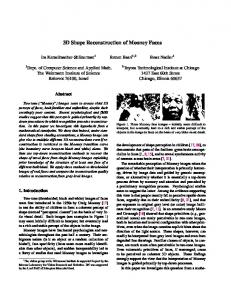
ization of 3D video are conducted in the 4D space (3D geometric + 1D temporal), we have to develop human-friendly 3D video editors and visualizers that help a user to understand dynamic events in the 4D space. This paper first describes an overall process of generating 3D video and then proposes a plane-based volume intersection method followed by its parallel pipeline implementation using a PC cluster2 . With this method, a temporal series of full 3D voxel representations of the object behavior can be obtained in real-time. Several results of its quantitative performance evaluation are given to demonstrate its effectiveness. In the latter half of the paper, we present an algorithm of generating video texture on the reconstructed dynamic 3D object surfaces. We first describe a naive view-independent rendering method and show its problems. Then, we improve the method by introducing image-based rendering techniques. Experimental results demonstrate the effectiveness of the improved method in generating high fidelity object images from arbitrary viewpoints3 . II. BASIC M ETHOD OF 3D V IDEO G ENERATION Figure 1 illustrates the basic process of generating a 3D video frame in our system: 1) Synchronized Multi-View Image Acquisition: A set of multi-view object images are taken simul2 3

An earlier version was published in ISPA03 [1]. An earlier version was published in 3DPVT 2002 [2].

taneously by a group of distributed video cameras (Figure 1 top row). 2) Silhouette Extraction: Background subtraction is applied to each captured image to generate a set of multi-view object silhouettes (Figure 1 second top row). 3) Silhouette Volume Intersection: Each silhouette is back-projected into the common 3D space to generate a visual cone encasing the 3D object. Then, such 3D cones are intersected with each other to generate the voxel representation of the object shape (Figure 1 third bottom). 4) Surface Shape Computation: The discrete marching cubes method [18] is applied to convert the voxel representation to the surface patch representation and then, the surface patch is deformed to increase the accuracy of the reconstructed 3D shape [19] (Figure 1 second bottom). 5) Texture Mapping: Color and texture on each patch are computed from the observed multi-view images (Figure 1 bottom). By repeating the above process for each video frame, we can create a live 3D motion picture. Note that in the current implementation, since the surface patch deformation requires large computation time (about a few minutes per frame) due to its naive iterative optimization process, the entire process above cannot run in realtime, while the 3D shape reconstruction and the texture mapping run in near video-rate respectively. In the following sections, we describe technical details of our real-time 3D shape reconstruction system and high fidelity video texture mapping algorithm. As for the surface mesh deformation to increase the 3D shape accuracy, refer to [19]. III. R EAL -T IME DYNAMIC 3D O BJECT S HAPE R ECONSTRUCTION S YSTEM A. System Organization Figure 2 illustrates the hardware organization of our real-time active dynamic 3D object shape reconstruction system. It consists of • PC cluster: 30 node PCs (dual Pentium III 1GHz) are connected through Myrinet, an ultra high speed network (full duplex 1.28Gbps). PM library for Myrinet PC clusters [20] allows very low latency and high speed data transfer, based on which we can implement efficient parallel processing on the PC cluster. • Distributed active video cameras: Among 30 PCs, 25 have calibrated Fixed-Viewpoint Pan-Tilt (FVPT) cameras [21], for active object tracking and

3

1 2 Base Silhouette Base Slice Fig. 3.

Fig. 2. PC cluster for real-time active dynamic 3D object shape reconstruction system.

image capturing. In the FV-PT camera, the projection center stays fixed irrespectively of any camera rotations, which greatly facilitates real-time active object tracking and its 3D shape reconstruction in a wide spread area [16]. We employ volume intersection [23] [24] [25] [26] [27] [28] as a basic computational algorithm to obtain the 3D shape of the object. This is because it can compute the full 3D object shape by well defined geometric computations, while stereo methods involve difficult matching processes as well as can generate only partial 2.5D shape. As is well known, however, the 3D shape reconstructed by the volume intersection is just an approximation. To increase the accuracy of the reconstructed 3D shape, [29] proposed the space carving method, where photometric information as well as multi-view silhouettes are employed. In [19], we proposed a deformable 3D mesh model to reconstruct an accurate 3D object shape by integrating object silhouettes, photometric properties, and 3D motion flows computed from multi-view video data. Here we confine ourselves to the problem of how to realize real-time volume intersection. Since the volume intersection involves a considerable amount of arithmetic operations, many methods for its efficient computation have been proposed. [23], [28] and [7] employed octree-based volume intersection methods. [13], on the other hand, proposed an image-based volume intersection, where a 2.5D depth map from an arbitrary viewpoint is generated by projecting and intersecting multi-view object silhouettes on the image plane corresponding to that viewpoint. To realize efficient volume intersection, we first developed the plane-based volume intersection method, where the 3D voxel space is partitioned into a group of parallel planes and the cross-section of the 3D object volume on each plane is reconstructed. Secondly, we devised the Plane-to-Plane Perspective Projection (PPPP)

Plane-based volume intersection method

algorithm to realize efficient plane-to-plane projection computation. Thirdly, to realize real-time processing, we implemented parallel pipeline processing on a PC cluster system. In what follows, we describe these methods in details.

B. Plane-based Volume Intersection Method Figure 3 illustrates the plane-based volume intersection method. For each camera, an object silhouette is first projected onto a common base plane to generate a base silhouette, which then is mapped onto the other planes (Figure 3 left). The cross-section of the object on each plane can be obtained by calculating the 2D intersection among the projected silhouettes (Figure 3 right). This plane-to-plane back-projection (homography) [30] is computationally less expensive than general 3D perspective projection: •

General perspective projection from 3D point (X, Y, Z) to 2D point (x1 /x3 , x2 /x3 ) can be represented by the following equation: 

x1





p11 p12 p13 p14 p22 p23 p24 p31 p32 p33 p34

    x2  =  p21

x3

•





X   Y   Z 1

   . 

(1)

This transformation requires 9 additions, 9 multiplications, and 2 divisions. In the case of the plane-to-plane projection, where the source 3D point is constrained on a 2D plane, the projection equation is simplified to the following equation: 









X h11 h12 h13 x1       x2  =  h21 h22 h23   Y  . 1 h31 h32 h33 x3

(2)

This requires 6 additions, 6 multiplications, and 2 divisions per point. To accelerate the plane-to-plane projection computation further, we developed the following algorithm.

4

B C AB

CC

DP lan

o

e

B C A C

B C

-w ear

C o

ise PP PP

A P o

Base Plane

A C Fig. 5.

Fig. 4.

Translation + Scaling (Plane-wise PPPP)

Lin

P

Linear PPPP algorithm

C. Accelerated PPPP Algorithm Based on the geometric relations between a pair of planes involved in the projection, the acceleration of the PPPP algorithm can be done in the following two ways: 1) For planes which are not parallel, we devised the linear PPPP algorithm (Figure 4). 2) For parallel planes, we apply the plane-wise PPPP algorithm(Figure 5). As will be described below, both algorithms consist of simple linear computations, which can be executed efficiently by popular graphics hardware. Linear Plane-to-Plane Perspective Projection In Figure 4, we want to map a silhouette on plane T A onto B , where A and B are not parallel. A B denotes the intersection line between the planes and O the center of perspective projection. Let P denote the T line that is parallel to A B and passing O. Then, take any plane including P (C in Figure 4), the image data T T on the intersection line A C is projected onto B C . As shown in the right part of Figure 4, this linear (i.e. line-based) perspective projection can be computed by a T T scaling operation, since A C and B C are parallel to each other. By rotating plane C around line P , we can map the entire 2D image on A onto B . In [6], we analyzed the computational complexity of this linear PPPP method and showed its computational efficiency. [13] employed a similar plane-based projection method to map a silhouette on an image plane to another and proved its computational efficiency. The difference between their method and our method rests in that (1) we reconstruct full 3D shape while [13] generates a 2.5D depth map for a specified viewpoint and (2) we T employ the intersecting line A B to linearize the planeto-plane projection while [13] used a group of epipolar lines. Plane-wise Plane-to-Plane Perspective Projection As shown in Figure 5, the projection between two parallel planes is simplified to 2D isotropic scaling and

Plane-wise PPPP

translation:

"

x1 x2

#

"

X =s Y

#

"

+

tx ty

#

,

(3)

where s represents the scaling and (tx , ty ) the translation vector. Equation (3) shows that this transformation requires 2 additions and 2 multiplications per point. Since this transformation is a pure 2D geometric transformation, 2D image processing hardware can be employed to accelerate the computation. To realize real-time 3D shape reconstruction, we next propose a parallel pipeline processing method for the above mentioned plane-based volume intersection. D. Parallelized Volume Intersection Method The process of the plane-based volume intersection method can be divided into the following stages: 1) Back-projection a) Projection from the image plane of each camera onto the common base plane (Linear PPPP) b) Projection from the base plane to the other parallel planes (Plane-wise PPPP) 2) Silhouette intersection on each plane To make this processing parallel on our PC cluster, we observe: • Since the process a) of stage 1 is closely connected with image capturing and silhouette extraction processes, it should be executed on the same PC that captures an image. • Since the silhouette intersection on each plane can be done independently of that on the others, we partition a set of parallel planes into a group of subsets and assign a subset to each PC, which computes the silhouette intersection on each plane included in its assigned subset. • To realize the above parallel silhouette intersection, we have to make each PC have a full set of multiview silhouettes. That is, after computing its own

5 Captured Image

SIP

SIP

SIP

BPP

BPP

BPP

Silhouette Image Base Plane Silhouette Image

Communication

PPP

Loop

PPP

Loop

PPP

Loop

Silhouette on a slice INT

INT

INT

Fig. 7.

Object Area on a slice

Final Result node1

node2

node3

Fig. 6. Processing flow of the parallel pipelined 3D shape reconstruction.

base plane silhouette, each PC broadcasts that data to all the other PCs. As will be proved later, this broadcasting does not introduce large overhead, because the data size transmitted is small (i.e. 2D bit image data representing the base plane silhouette) and the network speed is very high. Note that this silhouette duplication enables completely parallel silhouette intersection on the planes without any overhead. Figure 6 illustrates the processing flow of the parallel pipelined 3D shape reconstruction. It consists of the following five stages: 1) Image Capture : Triggered by a capturing command, each PC with a camera captures a video frame (Figure 6 top row). 2) Silhouette Extraction : Each PC with a camera extracts an object silhouette from the video frame (Figure 6 second top row). 3) Projection to the Base-Plane : Each PC with a camera projects the silhouette onto the common base-plane in the 3D space (Figure 6 third top row). 4) Base-Plane Silhouette Duplication : All base-plane silhouettes are duplicated across all PCs over the network so that each PC has the full set of all baseplane silhouettes (Figure 6 forth top row). Note that the data are distributed over all PCs in the system (i.e. PCs with and without cameras). 5) Object Cross Section Computation : Each PC computes object cross sections on specified parallel planes in parallel (Figure 6 three bottom rows). In addition to the above parallel processing, we introduced pipeline processing on each PC: 5 stages (corresponding to the 5 steps above) for a PC with

Average computation time for each pipeline stage.

a camera and 2 stages (the step 4 and 5) for a PC without a camera. In this pipeline processing, each stage is implemented as a concurrent process and processes data independently of the other stages. Note that since a process on the pipeline should be synchronized with its preceding and succeeding processes and, moreover, the stage 5 silhouette intersection cannot be executed until all silhouette data are prepared, the output rate (i.e. the rate of the 3D shape reconstruction) is limited to the rate of the slowest stage. E. Performance Evaluation In the experiments of the real-time 3D volume reconstruction, we used 6 digital IEEE1394 cameras (SONY DFW-VL500) placed at the ceiling (like Figure 2) for capturing multi-view video data of a dancing human. We will discuss their synchronization method later. The size of input image is 640 × 480 pixels and we measured the time taken to reconstruct one 3D shape in the voxel size of 2cm× 2cm× 2cm contained in a space of 2m × 2m × 2m. In the first experiment, we analyzed processing time spent at each pipeline stage by using 6 - 10 PCs for computation. Figure 7 shows the average computation time 4 spent at stages “Silhouette Extraction”, “Projection to the Base-Plane”, “Base-Plane Silhouette Duplication” and “Object Cross Section Computation”. Note that the image capturing stage is not taken into account in this experiment and will be discussed later. From this figure, we can observe the following: • The computation time for the Projection to the Base-Plane stage is about 18ms, which proves the accelerated PPPP algorithm is very efficient. To verify the computational efficiency of the accelerated PPPP algorithm, we replaced it with a 4

For each stage, we calculated the average computation time of 100 video frames on each PC. The time shown in the graph is the average time for all PCs.

6

(a) Soft Trigger Fig. 8.

•

•

•

Performance of the accelerated PPPP algorithm.

naive silhouette projection method, where an object silhouette in an image plane is projected onto the base plane pixel by pixel. Figure 8 compares the average computation time spent at each pipeline stage between 6 PCs with the accelerated PPPP (left) and 6–12 PCs with the naive projection (right). In all cases we used 6 cameras. This figure shows that the accelerated PPPP algorithm plays a crucial role in realizing real-time processing. Note that in the latter cases, the silhouette duplication stage was also elongated considerably. The reason for this may be that the thread scheduling for the pipeline processing introduced additional overheads since the base silhouette projection stage took a very long time compared with the other stages. As is shown in the leftmost bars in Figure 7, with 6 PCs (i.e. with no PCs without cameras), the bottleneck for real-time 3D shape reconstruction rests at the Object Cross Section Computation stage, since this stage consumes most computation time (i.e. about 40ms). By increasing the number of PCs, the time taken for that most expensive stage decreases considerably, while slightly increasing the data duplication overhead (the right part of Figure 7). This proves the proposed parallelization method is effective. With more than 8 PCs, we can realize video-rate 3D shape reconstruction.

In the second experiment, we measured the total throughput of the system including the image capturing process by changing the numbers of cameras and PCs. Figure 9 shows the throughput5 to reconstruct one 3D shape. In our PC cluster system, we developed two methods for synchronizing multi-view video capturing: use an 5 The time shown in the graph is the average throughput for 100 frames.

(b) Hard Trigger Fig. 9.

Computation time for reconstructing one 3D shape.

external trigger generator (Hard Trigger) and control the cameras through network-communication (Soft Trigger). From Figure 9 we can get the following observations: • In both synchronization methods, while the throughput is improved by increasing PCs, it saturates at a constant value in all cases: 80 ∼ 90ms in both methods. • Comparing the hard and soft triggers, they show almost similar performance. Since as was proved in the first experiment, the throughput of the computation itself is about 30ms, the elongated overall throughput is due to the speed of the image capture stage as well as the overhead involved in the process synchronization during the pipeline processing. That is, although a camera itself can capture images at a rate of 30 fps individually, the image capture synchronization reduces its frame rate down by half. This is partly because the external hard and soft triggers for synchronization are not synchronized with the internal hardware cycle of the camera and partly because it takes some time to synchronize PCs and transfer image data to PC memory: • First of all, the camera we use (SONY DFWVL500) reduces its frame rate down to 15 fps in

7

Fig. 11. Fig. 10. voxels.

Voxel representations of a 3D object behavior

Performance evaluation in the case of 1cm× 1cm× 1cm

the external hardware trigger mode. This is a major reason why the overall throughput is reduced in the hard trigger method. • In the soft trigger method, since the actual image capturing is done based on the internal clock of each camera, the capturing timing varies from PC to PC slightly (i.e. at most 33msec). This internal clock driven image capturing also introduces a delay between the capturing command issued by a PC and the actual image capturing. Note that the hard trigger guarantees the exactly synchronized image capturing. • We use the isochronous data transfer mode of IEEE 1394 and a Linux device driver, which introduce some overheads for synchronized image data transfer via IEEE 1394 line and buffering in the driver software. In the third experiment, we increased the resolution: 1cm× 1cm× 1cm voxels in a space of 2m × 2m × 2m. Figure 10 illustrates the overall throughputs for 6 PCs at the 2cm voxel resolution (left) and 8–24 PCs at the 1cm voxel resolution (right). In all cases we used 6 cameras. While we can speed up the computation by increasing PCs, it will not possible to realize over 10 volume per second with the current system at the resolution of 1cm voxels. In summary, the experiments proved the effectiveness of the proposed real-time 3D shape reconstruction system: the plane-based volume intersection method, its acceleration algorithm, and the parallel pipeline implementation. Moreover, the proposed parallel processing method is flexible enough to scale up the system by increasing numbers of cameras and PCs. While we used off-the-shelf devices, we have to develop sophisticated video capturing hardware including cameras to realize video-rate 3D shape reconstruction. To increase the voxel resolution, we have to employ faster PCs and/or make full use of graphics hardware.

(a)

(b)

Fig. 12. (a) surface patch model generated by the discrete Marching cube method and (b) surface patch model after deformation

IV. H IGH F IDELITY T EXTURE M APPING A LGORITHM Figure 11 illustrates snapshots of 3D voxel data of a dancing person at the resolution of 1cm × 1cm × 1cm reconstructed by the above described system. Then we apply to each voxel data the discrete marching cubes method [18] to convert the 3D object shape into the triangular patch representation. Figure 12(a) illustrates a close-up of the generated triangular patch data. As is well known and obvious from this figure, the 3D shape generated is not smooth and its concave parts (e.g. neck) are not well reconstructed. To solve these problems, we developed a deformable 3D mesh model, which uses photometric and motion information as well as multiview silhouettes [19]. Figure 12(b) illustrates the result of the deformation, where a more accurate and smooth 3D object shape is obtained. Since the currently implemented deformation program requires large computation time (about a few minutes per frame) due to its naive iterative optimization process and a large number of vertices (i.e. 12,000 – 15,000 vertices per volume at 1cm voxel resolution), the realtime processing is broken down at this stage and the subsequent texture mapping process is done as postprocessing, even if the mapping itself runs almost in real-time by a PC with a modern graphics engine.

8

In this section, we propose a novel texture mapping algorithm to generate high fidelity 3D video. The problem we are going to solve here is how we can generate high fidelity object images from arbitrary viewpoints based on the 3D object shape with limited accuracy. [3] first mapped each surface patch back to multi-view images to obtain multi-view textures for each patch and then took a weighted average of those textures. As will be described later, such view-independent patch-based texture mapping introduces jitters due to inaccurate 3D object shape and/or misalignments involved in the camera calibration. On the other hand, [11] [13] employed image-based rendering methods to generate arbitrary view images based on 3D shape data reconstructed from multi-view images, where a virtual view direction is specified to control the blending process of multi-view images. While such image-based rendering methods can avoid jitters in generated images, image sharpness is degraded due to the blending operation. In what follows, we first describe a naive rendering method which is similar to [3] and show problems in a view-independent patch-based rendering method. Then, we improve the method by introducing image-based rendering techniques. A. Naive Algorithm: Viewpoint Independent PatchBased Method We first implemented a naive texture mapping algorithm, which selects the most ”appropriate” camera for each patch and then maps onto the patch the texture extracted from the image observed by the selected camera. Since this texture mapping is conducted independently of the viewer’s viewpoint of 3D video, we call it the Viewpoint Independent Patch-Based Method (VIPBM). Algorithm (Figure 13) 1) For each patch pi , do the following processing. 2) Compute the locally averaged normal vector Vlmn using normals of pi and its neighboring patches. 3) For each camera cj , compute viewline vector Vcj directing toward the centroid of pi . 4) Select such camera c∗ that the angle between Vlmn and Vcj becomes maximum. 5) Extract the texture of pi from the image captured by camera c∗ . This method generates a fully textured 3D object shape, which can be viewed from arbitrary viewpoints with ordinary 3D graphics display systems. Moreover, its data size is very compact compared with that of the original multi-viewpoint video data.

cj

Vlmn

pi ck Fig. 13.

cl

Viewpoint independent patch-based method

c1 Vc -> p

Vc -> p 1

n

i

object

pi

Vc -> p 2

c2 Fig. 14.

cn

i

Np

Vc -> p

i

j

i

Veye -> p

i

i

cj

Viewpoint and camera position

From the perspective of fidelity, however, the displayed image quality is not satisfying: 1) Due to the rough quantization of patch normals, the best camera c∗ for a patch varies from patch to patch even if they are neighboring. Thus, textures on neighboring patches are often extracted from those images captured by different cameras (i.e. viewpoints), which introduces jitters in displayed images. 2) Since the texture mapping is conducted patch by patch and their normals are not accurate, textures of neighboring patches may not be smoothly connected. This introduces jitters at patch boundaries in displayed images. To overcome these quality problems, we developed a viewpoint dependent vertex-based texture mapping algorithm. In this algorithm, the color (i.e. RGB value) of each patch vertex is computed taking into account the viewpoint of a viewer, and then the texture of each patch is generated by interpolating the color values of its three vertices. B. Viewpoint Dependent Vertex-Based Texture Mapping Algorithm (1) Definitions First of all, we define words and symbols as follows (Figure 14), where bold face symbols denote 3D position/direction vectors:

9

pi

pk

i

cj Fig. 15.

i i i i i i i i i

kj i i i i i i i

k k k i i i i i

k k k k i i i i

vertices in type (1) and (2) are visible, while in type (5) three vertices of the occluded patch are not visible. In type (3) and (4), only some vertices are visible. RGB values I(vpki ,cj ) of the visible vertex v kpi ,cj are computed by

k k k k k k k i k i i

I(vpki ,cj ) = Icj (ˆ vpi ,cj ),

depth

(5)

where Icj (v) shows RGB values of pixel v on the image ˆ pki ,cj denotes the pixel captured by camera cj , and v position onto which the vertex vpki ,cj is mapped by the imaging process of camera cj .

Depth buffer

Type (1)

Type (2)

Type (4)

Fig. 16.

i i i i

i i i i i i i

Type (3)

Type (5)

Relations between patches

a group of cameras: C = {c1 , c2 , . . . , cn } a viewpoint for visualization: eye • a set of surface patches: P = {p1 , p2 , . . . , pm } • outward normal vector of patch pi : npi • a viewing direction from eye toward the centroid of pi : v eye→pi • a viewing direction from cj toward the centroid of pi : v cj →pi (k = 1, 2, 3) • vertices of pi : vk pi k • vertex visible from cj (defined later): vp i ,cj k k • RGB values of vpi ,cj (defined later): I(vp ) i ,cj • a depth buffer of cj : Bcj Geometrically this buffer is the same as the image plane of camera cj . Each pixel of Bcj records such patch ID that is nearest from cj as well as the distance to that patch from cj (Figure 15). When a vertex of a patch is mapped onto a pixel, its vertex ID is also recorded in that pixel. (2) Visible Vertex from Camera cj The vertex visible from cj , vpki ,cj , is defined as follows. 1) The face of patch pi can be observed from camera cj , if the following condition is satisfied. •

•

npi · v cj →pi < 0

(4)

2) vpki is not occluded by any other patches. Then, we can determine vpki ,cj by the following process: 1) First, project all the patches that satisfy equation (4) onto the depth buffer Bcj . 2) Then, check the visibility of each vertex using the buffer. Figure 16 illustrates possible spatial configurations between a pair of patches: all the

(3) Algorithm 1) Compute RGB values of all vertices visible from each camera in C = {c1 , c2 , . . . , cn }. 2) Specify the viewpoint eye. 3) For each surface patch pi ∈ P , do 4 to 9. 4) If v eye→pi · npi < 0, then do 5 to 9. 5) Compute weight wcj = (v cj →pi ·v eye→pi )m , where m is a weighting factor to be specified a priori. 6) For each vertex vpki (k = 1, 2, 3) of patch pi , do 7 to 8. 7) Compute the normalized weight for vpki by wck w ¯ckj = P j k . l wcl

(6)

Here, if vpki is visible from camera cj , then wckj = wcj , else wckj = 0. 8) Compute the RGB values I(vpki ) of vpki by I(vpki )

=

n X

w ¯ckj I(vpki ,cj )

(7)

j=1

9) Generate the texture of patch pi by linearly interpolating RGB values of its vertices. To be more precise, depending on the number of vertices with non-zero RGB values, the following processing is conducted: • 3 vertices: Generate RGB values at each point on the patch by linearly interpolating the RGB values of 3 vertices . • 2 vertices: Compute mean values of the RGB values of the 2 vertices, which is regarded as those of the other vertex. Then apply the linear interpolation on the patch. • 1 vertex: Paint the patch by the RGB values of the vertex. • no vertex: Texture of the patch is not generated: painted by black for example. By the above process, an image representing an arbitrary view (i.e from eye) of the 3D object is generated.

10 #5

#1 #8 #9 #4

#2 #6

#11

#7 #3

#1 #12

#10 250 cm 400 cm 450 cm

Fig. 17.

Camera Setting

VDVBM–1

VDVBM–2

VIPBM

Original sequence

Frame # 103

Cam 5

Cam 11

Fig. 18. Cropped images generated by VDVBM–1, VDVBM–2, VIPBM, and original sequence

C. Performance Evaluation To evaluate the performance of the proposed viewpoint dependent vertex-based method (VDVBM), we first compare it with the viewpoint independent patchbased method (VIPBM) qualitatively. Figure 18 compares those images generated by VDVBM-1, VDVBM2 and VIPBM with an original video image. Note that to evaluate the performance of VDVBM, we employed two methods: VDVBM–1 generates images including real images captured by camera cj = eye itself (i.e. cam 5 and 11 in Figure 18, respectively), while VDVBM–2 excludes such real images captured by camera cj . We can observe that VIPBM introduces many jitters in images, which are considerably reduced by VDVBM.

Then, we conducted quantitative performance evaluations. That is, we calculate RGB root-mean-square (rms) errors between a real image captured by camera cj = eye and its corresponding images generated by VIPBM, VDVBM–1, and VDVBM–2, respectively. The experiments were conducted under the following settings: • camera configuration: Figure 17 • image size: 640×480[pixel] 24 bit RGB color • viewpoint (eye): camera 5 • weighting factor in VDVBM: m = 5 Figure 20 illustrates the experimental results, where rms errors for frame 95 to 145 are computed. This figure shows that VDVBM performs better than VIPBM. The superiority of VDVBM and its high fidelity image generation capability can be easily observed in Figure 19, where real and generated images for frame 110 and 120 are illustrated. Next, we tested how we can improve the performance of VDVBM by increasing the spatial resolution of the 3D object surface patch data. Figure 21 shows the method of subdividing a patch into three (S3) and six (S6) subpatches to increase the spatial resolution. We examine the average side length of a projected patch on the image plane of each camera by projecting original and subdivided 3D surface patches onto the image plane. Figure 22 shows the mean side length of the patches projected on the image plane of each camera. Note that since camera 9 is located closer to the 3D object (see Figure 17), object images captured by it become larger than those by the other cameras, which caused bumps (i.e. larger side length in pixel) in the graphs in Figure 22. We can observe that the spatial resolution of S6 is approximately the same as that of an observed image (i.e. 1 pixel). That is, S6 attains the finest resolution, which physically represents about 5mm on the object surface. To put this another way, we can increase the spatial resolution up to six sub-divisions, which improves the quality of images generated by VDVBM. To quantitatively evaluate the quality achieved by using subdivided patches, we calculated root-mean-square errors between real images and images generated by VDVBM-1 with the original patches, S3, and S6, respectively (Figure 23). Figure 23 shows that subdividing patches does not numerically reduce the errors. The reason of this observation is as follows. Figure 24 shows the spatial distribution of the color difference between a real image and a generated image, from which we can see that large errors arise around the object contour and texture edges. These errors are difficult to reduce by

11

VDVBM–1

VDVBM–2

VIPBM

Original sequence Frame # 110 Fig. 19.

Frame # 120

Sample images of 3D video generated by VDVBM–1, VDVBM–2, and VIPBM from eye = cam 5 in Figure 17. 75 VDVBM-1 VDVBM-2 VIPBM 70

Root-mean-square error

65

An original patch

A patch subdivided

A patch subdivided

into three (S3)

into six (S6)

60

55

Fig. 21.

Subdivision of a 3D surface patch

50

45

40

35 95

100

105

110

115

120

125

130

135

140

145

Frame number

Fig. 20.

Root-mean-square error of RGB value (1)

subdividing patches because they come from motion blur, the misalignment of the camera calibration, or the asynchronization by the soft trigger image capturing. Fidelity of images generated with subdivided patches, however, is improved in smooth object surface areas (Figure 25). Thus, subdividing patches is effective from

a fidelity point of view. Note that the zigzag patterns in Figures 20 and 23 were caused due to the imperfectness of the synchronization of the image capturing process. Since we used the soft trigger mode to capture multi-view video data in this experiment, the image capture timing varied slightly PC by PC. This timing deviation sometimes increased the inaccuracy of the reconstructed 3D shape, because the dancer moved her hands rather fast. Finally, we show examples generated by VDVBM– 1 with subdivided patches (S6) viewed from camera 5, 11, and an intermediate point between them (Figure 26).

12 5 4.5

’Original’ ’Subdivided into 3’ ’Subdivided into 6’

4

pixel

3.5 3 2.5 2 1.5 1

cam1

cam2

cam3

cam4

cam5

cam6

cam7

cam8

cam9 cam10 cam11 cam12

camera

Fig. 22. Mean side length (in pixel) of patches projected on the image plane of each camera. 38

’Original’ ’Subdivided into 3’ ’Subdivided into 6’

37

Root-mean-square error

Fig. 24. Color difference between a real image and a generated image (frame #106)

36

35

34

33

32

31 95

Original 100

105

110

115

120

125

130

135

140

Fig. 23.

Subdivided (S6)

145

Frame number

Root-mean-square errors of RGB value (2)

Figure 26 shows that the images generated by VDVBM look almost real even when they are viewed from the intermediate point of the cameras. For rendering 3D video data like Figure 26, we used a popular PC: (CPU: Xeon 2.2GHz, Memory: 1GB, Graphics Processor: GeForce 4 Ti 4600, Graphics library: DirectX 9.0b) and used the following two stage process: 1) First, compile a temporal sequence of reconstructed 3D shape data and multi-view video into a temporal sequence of vertex lists, where multiview RGB values are associated with each vertex. It took about 2.8 sec to generate a vertex list for a frame of 3D video. 2) Then, with the vertex list sequence, arbitrary VGA views of the 3D video sequence can be rendered at 6.7 msec/frame. Thus, we can realize real-time interactive browsing of 3D video with a PC. Note also that since we can render a pair of stereo images in real-time (i.e. 14 msec/stereo-pair), we can enjoy pop-up 3D image interactively with a 3D display monitor. V. C ONCLUSION 3D video records an object’s full 3D shape, motion, and surface texture. In this paper, we first proposed a

Fig. 25. Example images rendered with original and subdivided patches (frame #106)

real-time parallel pipeline volume intersection method on a PC cluster: the plane-based volume intersection method, its acceleration algorithm, and the parallel pipeline implementation. The quantitative performance evaluations demonstrated that the acceleration and parallelizing algorithms we proposed are very efficient and enabled us to reconstruct dynamic full 3D shape over 10 volume per sec at the a 2cm× 2cm× 2cm voxel resolution. In the latter half of the paper, we proposed a high fidelity texture mapping method. The qualitative and quantitative performance evaluations demonstrated that the proposed texture mapping method can produce object images from arbitrary viewpoints in almost the same quality as real video data. As listed in the introduction, to make 3D video usable in everyday life, we still have to develop methods of • higher speed and more accurate 3D behavior reconstruction • 3D shape acquisition in a wide spread area and for multiple people • more natural image generation • effective data compression • editing 3D video for artistic image contents. This work was supported by the grant-in-aid for scientific research (A) 13308017. We are grateful to Real

13

Cam 5 Fig. 26.

Intermediate between cams 5 and 11

Cam 11

Visualized 3D video with subdivided patches (frame#103)

World Computing Partnership, Japan for allowing us to use their multi-viewpoint video data. R EFERENCES [1] X. Wu and T. Matsuyama: Real-Time Active 3D Shape Reconstruction for 3D Video, Proc. of 3rd International Symposium on Image and Signal Processing and Analysis, pp.186–191, 2003. [2] T. Matsuyama and T. Takai: Generation, Visualization, and Editing of 3D Video, Proc. of symposium on 3D Data Processing Visualization and Transmission, pp.234–245, 2002. [3] S. Moezzi, L. Tai, and P. Gerard: Virtual View Generation for 3D Digital Video, IEEE Multimedia, pp.18–26, 1997. [4] G. Cheung and T. Kanade: A Real Time System for Robust 3D Voxel Reconstruction of Human Motions, Proc. of CVPR, pp.714–720, 2000. [5] T. Kanade, P. Rander, S. Vedula, and H. Saito: Virtualized Reality: Digitizing a 3D Time-Varying Event as is and in Real Time, in Mixed Reality (Y.Ohta and H.Tamura eds.), pp.41–57, Ohmsha, 1999. [6] T. Wada, X. Wu, S. Tokai, T. Matsuyama: Homography Based Parallel Volume Intersection: Toward Real-Time Reconstruction Using Active Camera: Proc. of Computer Architectures for Machine Perception, pp.331–339, 2000. [7] E. Borovikov and L. Davis: A Distributed System for RealTime Volume Reconstruction, Proc. of Computer Architectures for Machine Perception, pp.183–189, 2000. [8] T. Kanade, A. Yoshida, K. Oda, H. Kano, and M. Tanaka: A Stereo Machine for Video-Rate Dense Depth MApping and its New Applications, Proc. of Computer Vision and Pattern Recognition, pp.196–202, 1996. [9] J. Mulligan, V. Isler, and K. Daniilidis: Trinocular Stereo: A Real-Time Algorithm and its Evaluation, International Journal of Computer Vision, Vol.47, No.1/2/3, pp.51–61, 2002. [10] H. Hirschmuller, P. R. Innocent, and J. Garibaldi: Real-Time Correlation-Based Stereo Vision with Reduced Border Errors, International Journal of Computer Vision, Vol.47, No.1/2/3, pp.229–246, 2002. [11] T. Naemura, J. Tago, and H. Harashima: Real-time video-based modeling and rendering of 3D scenes, IEEE Computer Graphics and Applications, Vol.22, pp.66–73, 2002. [12] P. Kauff and O. Schreer: An immersive 3d video-conferencing system using shared virtual team user environments, Proc. of ACM Conf. on Collaborative Virtual Environments, pp.105–112, 2002. [13] W. Matusik, C. Buehler, R. Raskar, S. Gortler, and L. MacMillan: Image-Based Visual Hulls, Proc. of SIGGRAPH, pp.369– 374, 2000. [14] H. Baker, D. Tanguay, I. Sobel, D. Gelb, M. Gross, W. Culbertson, and T. Malzbender: The coliseum immersive teleconferencing system, Proc. of International Workshop on Immersive Telepresence, 2002.

[15] M. Turk and G. Robertson: Perceptual User Interfaces, Communications of ACM, VOl.43, No.3, pp.33–34, 2000. [16] T. Matsuyama and N. Ukita: Real-Time Multi-Target Tracking by a Cooperative Distributed Vision System, Proc. of IEEE, Vol.90, No.7, pp.1136–1150, 2002. [17] T. Matsuyama and R. Yamashita: Requirements for Standardization of 3D Video, ISO/IEC JTC1/SC29/WG11, MPEG2002/M8107, 2002. [18] Y. Kenmochi, K. Kotani, A. Imiya: Marching Cubes Method with Connectivity Consideration: PRMU–98–218, pp.197–204, 1999 (in Japanese). [19] S. Nobuhara and T. Matsuyama: Dynamic 3D Shape from Multi-Viewpoint Images Using Deformable Mesh Model, Proc. of 3rd International Symposium on Image and Signal Processing and Analysis, pp.192–197, 2003. [20] H. Tezuka, A. Hori, Y. Ishikawa, and M. Sato: PM: An Operating System Coordinated High Performance Communication Library, High-Performance Computing and Networking (P. Sloot and B. Hertzberger, eds.), Lecture Notes in Computer Science, Vol.1225, pp.708–717. Springer-Verlag, 1997. [21] T. Wada and T. Matsuyama: Appearance Sphere:Background Model for Pan-Tilt- Zoom Camera, Proc. of 13th ICPR, pp.A718–A-722, 1996. [22] T. Matsuyama: Cooperative Distributed Vision – Dynamic Integration of Visual Perception, Action, and Communication –, Proc. of Image Understanding Workshop, pp. 365–384, 1998 [23] M. Potmesil. Generating Octree Models of 3D Objects from their Silhouettes in a Sequence of Images. Computer Vision,Graphics, and Image Processing, 40: pp.1–29, 1987. [24] W. N. Martin and J. K. Aggarwal. Volumetric Description of Objects from Multiple Views. IEEE Transactions on Pattern Analysis and Machine Intelligence, 5(2): pp.150–158, 1987. [25] A. Laurentini: The Visual Hull Concept for Silhouette Based Image Understanding IEEE Transactions on Pattern Analysis and Machine Intelligence, 16(2): pp.150–162, 1994. [26] A. Laurentini: How Far 3D Shapes can be Understood from 2D Silhouettes, IEEE Transactions on Pattern Analysis and Machine Intelligence, 17(2): pp.188–195, 1995. [27] P. Srivasan, P. Liang, and S. Hackwood: Computational Geometric Methods in Volumetric Intersections for 3D Reconstruction, Pattern Recognition, 23(8): pp.843–857, 1990. [28] R. Szeliski. Rapid Octree Construction from Image Sequences, CVGIP: Image Understanding, 58(1): pp.23–32, 1993. [29] K. N. Kutulakos and S. M. Seitz. A theory of shape by space carving, IEEE International Conference on Computer Vision, pp.307–314, 1999. [30] J. Semple and G. Kneebone: Algebraic Projective Geometry, Oxford Science Publication, 1952.