Real-Time Semi-Automatic Segmentation Using a ... - IEEE Xplore

Real-Time Semi-Automatic Segmentation Using a Bayesian Network Eric N. Mortensen Oregon State Univ. [email protected]

Jin Jia Microsoft

Abstract This paper presents a semi-automatic segmentation technique called Bayesian cut that formulates object boundary detection as the most probable explanation (MPE) of a Bayesian network’s joint probability distribution. A two-layer Bayesian network structure is formulated from a planar graph representing a watershed segmentation of an image. The network’s prior probabilities encode the confidence that an edge in the planar graph belongs to an object boundary while the conditional probability tables (CPTs) enforce global contour properties of closure and simplicity (i.e., no self-intersections). Evidence, in the form of one or more connected boundary points, allows the network to compute the MPE with minimal user guidance. The constraints imposed by CPTs also permit a linear-time algorithm to compute the MPE, which in turn allows for interactive segmentation where every mouse movement recomputes the MPE based on the current cursor position and displays the corresponding segmentation.

1. Introduction Image segmentation is a fundamental problem in computer vision. No fully automatic technique exists that correctly identifies objects in a general class of images. Many general image segmentation tasks will continue to require some amount of human intervention in order to identify the object(s) of interest. Thus, a goal of this work is to reduce the human effort required for accurate and reliable object definition. This work formulates boundary detection as a Bayesian network constructed from a watershed segmentation. The network’s topology and constraints enforce simple (no self-intersections), closed image contours. The MPE (most probable explanation) prior to evidence can produce multiple closed, non-intersecting contours (or loops). Clipping the probabilities normalizes the MPE’s path length and results in no loops unless an observation is provided by the user, in which case the MPE defines a single loop that includes the observed contour point(s). In addition to enforcing closure and simplicity, the network’s topology and constraints allow for a lineartime algorithm that computes the exact MPE. This linear time algorithm allows for extremely fast MPE computation such that every mouse movement provides

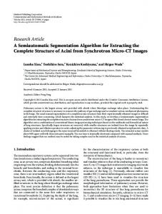
Figure 1: Example segmentations with Bayesian cut: Each contour is defined with a single observation (shown as a crosshair). The most probable contour is computed and displayed in real time for each new mouse position.

evidence to the Bayes net which in turn forces realtime recomputation and display of the segmentation. Figure 1 shows some objects whose boundaries are defined with just a single observation (by placing the mouse cursor close to the object boundary).

2. Background 2.1. Related Work Belief networks and other probabilistic graphical models have been applied to many computer vision problems [11,13,25]. Of particular relevance to this work are those methods that use belief networks (or similar Bayesian or statistical principles) for boundary detection. Elder and Zucker [7] develop a probabilistic model for object boundary detection in which maximum-likelihood contours are computed using a shortest path algorithm. It guarantees an exact solution in polynomial time, but favors the shortest loop and lacks global completeness and simplicity constraints. More recently, Elder et al. [8] combine prior probabilistic knowledge of an object’s appearance with models for contour grouping. They find candidate contours via a constructive search that does not guarantee optimality. They also use trained object-specific priors. Mahamud et al. [18] identifies smooth, closed contours by finding

Proceedings of the 2006 IEEE Computer Society Conference on Computer Vision and Pattern Recognition (CVPR’06) 0-7695-2597-0/06 $20.00 © 2006

IEEE

the eigenvector associated with the maximum eigenvalue of a transition matrix encoding a Markov process that expresses the conditional probability that any two edges belong to the same contour. Blake et al. [3] use a pseudo-likelihood algorithm to learn the color mixture and coherence parameters for a minimum graph cut (min-cut) model [4] in an interactive figure-ground segmentation application. Kumar et al. [15] simultaneously detect and segment images containing instances of specific object categories. They too use min-cut to solve a Markov random field (MRF) guided by global shape priors through a layered pictorial structure learned for a particular object category. Like this work, Li et al. [16] build a weighted regionadjacency graph (the dual of our graph) from a watershed segmentation and use min-cut to find the minimum Gibb’s energy. They also allow a user to adjust vertices of a boundary representation and then compute the pixel-based min-cut within a narrow band around the boundary. Rother et al. [22] develop an iterative graph cut optimization that simplifies user interaction and use a robust border matting to simultaneously determine an object matte and foreground color.

We have not seen any active contour [14] or graph cut method [4] that satisfies the desired real-time and proactive criteria. While live-wire/scissors [9,19] and multi-level banded graph cuts [17] provide real-time feedback, they too are reactive rather than proactive. Further, scissors’ piece-wise contour construction imposes ordering constraints on the boundary definition, they don’t formulate segmentation within a probabilistic framework, and they don’t ensure the Gestalt principles of closure or simplicity. In developing a tool that satisfies the above criteria, we began with an oversegmented image and, to formulate segmentation within a probabilistic framework, constructed a belief network that maps onto this initial segmentation. We designed the network such that the MPE of the network’s joint probability distribution defines a segmentation that enforces the global Gestalt principles of closure and simplicity. In developing an efficient algorithm to compute the MPE, we discovered, to our surprise, that the closure and simplicity properties incorporated into the network allowed for a linear time solution to the exact MPE.

2.2. Developmental History

Belief (or Bayesian) networks are directed acyclic graphs where vertices represent random variables and arcs indicate a direct “causal” relationship between variables. A Bayes net is a probabilistic graphical model that restricts the graph to be directed and acyclic. Other models such as Markov random fields (MRFs) have no such restrictions.

This work grew out of a desire to apply belief networks to user-guided segmentation. We wanted a probabilistic segmentation method that was: • General purpose: it should segment a wide variety of objects and not just images containing objects from a small set of learned categories. • User-guided: since all fully automatic segmentation methods ultimately fail, in part or in whole, on a general class of images, a human needs to guide segmentation, ideally with minimal effort. • Real-time: user guidance requires that visual feedback occur in a timely fashion. Ideally, the segmentation should provide results during interaction so that each new input (e.g., pointer movement) supplies new information that forces immediate reevaluation and display of the results. • Proactive: rather than wait for the necessary input to satisfy initialization criteria (e.g., an approximate contour, a trimap, etc.), the method should immediately seek out and display a solution, and refine the results as new information is available. • Accurate: the result should be accurate enough for application to medical analysis or image editing (e.g., object cut and paste). Unfortunately, many previous user-guided methods produce results that literally cut corners/appendages and/or include background; thus necessitating additional user effort to produce a satisfactory segmentation.

3. Belief Network

3.1. Initial Undirected Graph Previous probabilistic graphical models create nodes for every pixel. Our network is mapped onto the region boundaries of a watershed segmentation [2,24]. The resulting “super-pixel” representation reduces the network size (resulting in faster inference) and allows the computed probabilities to incorporate both meaningful edge- and region-based measures. The watershed operates on the image’s gradient magnitude computed in CIE L*a*b* color space (using a multiscale gradient operator) where, to reduce the response to shadow edges, we weight the luminance component less. To facilitate mapping to a Bayesian network, we impose an undirected graph G = (V, E) on the resulting watershed lines. Vertices V = {v1, v2, …, vn} are placed where three or more watershed lines converge and edges E = {(vi, vj) | vi, vj ∈ V} form along a section of a watershed line connecting two vertices. We use a very efficient watershed implementation [10,20] where region boundaries, and thus graph edges, follow pixel cracks; as such, every pixel belongs to some region and each vertex (located at a pixel corner) is at most degree four. Figures 2(a-c) illustrates creation of the undirected graph.


IEEE

3.2. Bayesian Network A belief network is a pair (Γ, Π ) where Γ is a directed acyclic graph (DAG) that maps to our initial graph G and Π is a set of probability tables. The digraph Γ = (X, A) has a set of nodes X corresponding to random variables and a set of arcs A indicating conditional dependence. The node set X = XE ∪ XV is the union of “edge” variables XE = { X Ei, j | (vi, vj) ∈ E} and “vertex” variables XV = { X Vi | vi ∈ V} created from every edge and node in G, respectively. Note that since G is undirected, X Ei, j = X Ej, i . The arc set A = {( X Ei, j , X Vi ), ( X Ei, j , X Vj )) | vi, vj ∈ V, (vi, vj) ∈ E} has directed arcs from every “edge” node (E-node) X Ei, j to the two “vertex” nodes (V-nodes) X Vi and X Vj connected by that edge (vi, vj) in G. Figure 2(d) illustrates construction of Γ from the undirected graph in Fig. 2(c). The set of probability tables Π = Π E ∪ Π V is the union of prior E-node probability tables for the Enodes, ΠE = {P( X Ei, j ) | X Ei, j ∈XE}, and conditional probability tables (CPTs) for the V-nodes, ΠV = {P( X Vi | pai) | X Vi ∈ XV}, where pai = { X Ei, j | ( X Ei, j , X Vi ) ∈ A}

(2)

where two E-nodes are married if they are both parents to the same V-node. A loop is a cycle in G or a sequence of married E-nodes such that im = i1. A simple loop also requires that ij ≠ ik if j ≠ k. X Ei, j

3.2.1. Most Probable Explanation (MPE). Let = xi,j and X Vi = xi denote a boolean assignment (i.e., xi,j, xi ∈ {true, false}) to the random variable represented by an E-node and a V-node, respectively. The joint probability distribution (JPD) over X is given by P(x) =

∏ P ( xi, j ) ∏ P ( x i pai ) X

E

X

V

(b)

vi

X Vi

vj X Ei, j

(vi, vj)

X Vj

(c)

(3)

X Vj

(e)

IEEE

X Vi

Figure 2: Creation of the belief network: (a) Original image. (b) Watershed transform of gradient magnitude. (c) Zoomed section of (b) showing initial graph construction. (d) Belief network constructed from initial graph in (c). (e) Two-layer representation.

where x is an assignment of all random variables in X and pa i denotes the assignment to the parents of X Vi . The MPE is the assignment x that maximizes the JPD: MPE ( x

MPE

) = arg max P ( x ) . (4) x If there is evidence (i.e., some variables are observed or known) then the MPE is MPE ( y

MPE

e ) = arg max P ( y e ) . (5) y where the evidence e is the assignment of the set of observed variables E ⊂ X and y is an assignment of the remaining unknown variables Y = X − E. Taking the negative logarithm of Eq. (3), the MPE is then the assignment that minimizes § · – ln P ( x ) = – ln ¨ P ( x i, j ) P ( x i pa i ) ¸ V © XE ¹ X

∏

§ = – ¨ ln P ( x i, j ) + © XE

¦

∏

¦ X

V

· ln P ( x i pa i )¸ . ¹

(6)

3.2.2. Probability Tables. Since our goal is to find closed contours that correspond to object boundaries, the set of probability tables Π should: • Estimate the assurance that the graph elements correspond to object boundaries.


(d)

X Ei, j

(1)

is the parent set for V-node X Vi . The network is a planar DAG, but it’s also useful to view the network in two levels: the top level has the set of priors XE and the conditional variables XV are placed below (see Fig. 2(e)). “Edge” variables are parents to “vertex” variables since the V-nodes serve as constraint variables (i.e., observed to be true) that enforce simple closed contours (see Section 3.2.2). Bayesian inference often determines the posterior probability of unobserved variables from observed conditional variables. Since our goal is to determine the set of edges that form closed contours, our network is designed to infer the unobserved E-nodes from the known V-node constraints and any observed E-nodes. An image contour is represented as either a path in G or a sequence of married E-nodes ( X iE1, i2, X Ei 2, i3, X iE3, i4, …, X iEm – 2, im – 1, X iEm – 1, i m )

(a)

• Enforce closed contours with no self-intersections. • Be length invariant. We address each of these criteria in turn. Boundary assurance: we assign to each edge (vi, vj) ∈ E in G an “assurance” value a(vi, vj) = a(vj, vi) between 0 and 1 based on local edge and region information including gradient magnitude, local curvature, and a statistical similarity measure between the regions on either side of the edge [21]. Since various measures can be used effectively for a(vi, vj)—including a simple inverted, biased, and appropriately scaled gradient magnitude—the computational details of a(vi, vj) are not critical. Suffice it to say that a(vi, vj) should be closer to one for edges that are estimated to be on the object boundary and closer to zero for edges that are not. The E-node probability tables are computed from the initial edge assurances. Simplicity and closure: global simplicity and closure are enforced with local constraints built into each V-node’s conditional probability table (CPT). For V-node X Vi , let True

pa i

E

= { X Ei, j ∈ pa i x i, j = True }

(7)

be the set of parent E-nodes, X Ei, j , that have an assignment, E x i, j , of true. The CPT for a V-node is then given by True

1, if pa i = 0 or 2 P ( X Vi = True ) = ® ¯ 0, otherwise

(8)

where |•| denotes set rank. The probability that X Vi is true is unity iff exactly zero or two of its parent E-nodes are assigned to true and zero otherwise. Thus, the CPT for a degree three V-node has exactly 4 out of 8 non-zero entries while a degree four V-node has 7 out of 16 non-zero entries—including the case where all parent E-nodes are assigned to false. The non-zero entries specify valid configurations of adjacent E-nodes having a true assignment. Note that for a V-node to enforce simplicity and closure, non-zero entries only need be a constant value 0 > c ≥ 1. There are two conditions to enforcing global simplicity and closure: First, every V-node has non-zero probability of a true assignment only for CPT entries with exactly two parents on (i.e., with an assignment of true) or with no parents on. Second, the V-nodes are observed to be true, thereby constraining every V-node to enforce the first condition, namely that either zero or two of its parents are on. These constraints guarantee either no path or just one path through every V-node. Since a loop with no self-intersections is the only type of contour that satisfies these constraints, any assignment x that maximizes P( x ) must have either no loops or possibly multiple loops that do not intersect with themselves or each other. Since V-nodes are forced a priori to be true, all future discussion of evidence will refer only to observations about E-nodes. MPE If x produces no loops and we then observe a single MPE E-node to be true, the MPE assignment, y e , based on this new evidence will create a single loop. Thus, turning on just one E-node is sometimes sufficient to specify an

object’s boundary (as in Fig. 1). We refer to the closed conMPE tour resulting from y e as the most probable loop. For clarity, we define what we mean when a node is on or off. An E-node X Ei, j is on when it is either observed or assigned to be true and off when it is observed or assigned to be false. Since a V-node is constrained to be true, a Vnode is on when it has exactly two parents that are on and off when no parents are on (all other configurations are defined as impossible by the CPT). In other words, a Vnode is on if it’s included in a loop and off otherwise. Thus, for notational convenience we define the following: P Eon ( i, j ) = P ( X Ei, j = true ) P Eoff ( i, j ) = P ( X Ei, j = false ) = 1 – P Eon ( i, j ) and (allowing some notational sloppiness) P Von ( i, j, k ) = P ( X Vj = true X Ei, j, X Ej, k = true, pa j – { X Ei, j, X Ej, k } = false ) (10) P Voff ( j ) = P ( X Vj = true pa j = false ) Note that since valid (non-zero) V-node CPT entries are all the same value, then P Von ( i, j, k ) = P Voff ( j ) . Length invariance: Since E-nodes are priors, their probability tables have only one entry per possible assignment—in this case X Ei, j = true and X Ei, j = false. To overcome the tendency towards small loops, the probability of turning on “good” edges needs to be greater than or equal to the probability of keeping them off—i.e., we want E P ( X i, j = true ) ≥ 0.5 . We compute the probability that an edge is part of a path within its local neighborhood. The neighborhood of an edge (vi, vj) is defined as all the edges that are connected to the vertices vi and vj. The E-node probability is given by sum on ( i, j ) - a ( v i, v j ) (11) P ( X Ei, j = true ) = ----------------------------------------------------------sum on ( i, j ) + sum off ( i, j ) where ¦ a ( v k, vi ) + a ( vi, vj ) + a ( vj, vl ) ½¾ (12) ® E X ¿ ¯ ( l ≠ i ), j ∈ pa j ∈ pa

1 sum on ( i, j ) = --- ¦ 3 XEi, ( k ≠ j )

i

is the summed assurance of all neighborhood paths that include edge (vi, vj) and sum off ( i, j ) =

1 --- ¦ 2 X Ei, ( k ≠ j )

+

¦ a ( vk, v i ) + a ( v i, vl ) ½¾ ® E X ∈ pa i ¿ ∈ pa ¯ i, ( l < k ∧ l ≠ j ) i

IEEE

(13)

1 --- ¦ 2 X E( k ≠ i ), j

¦ a ( v k, vi ) + a ( vi, vl ) ½¾ ® E ¿ ∈ pa ¯ X ( l < k ∧ l ≠ i ), j ∈ pa j j

is the sum of all paths that do not include edge (vi, vj). Eq. (11) performs either maximal boosting or non-maximal suppression of the edge: if the edge is on a high assurance path relative to its neighborhood, its probability gets boosted; if not, it gets suppressed. To avoid boosting noise edges, we rescale the ratio by the edge’s initial assurance


(9)

value. The resulting E-node probabilities for strong edges are typically between 0.5 and 0.65. Just as probabilities below 0.5 favors shorter loops, probabilities above 0.5 favors longer loops. To achieve true length invariance, the probabilities for all “boundary” E-nodes in a loop should be exactly equal to 0.5. Clipping all true values at 0.5 thus ensures length invariance for loops with strong edge probabilities. However, rather than clip the probability table entries directly, we clip the log probabilities at zero when creating edge weights (see Section 4).

4.2. Graph Weights We create a weighted, planar graph by adding edge and vertex weights to the initial planar graph. Since an E-node is assumed to be off prior to any evidence, an edge weight we(vi, vj) corresponds to flipping an Enode from off to on and is given by P Eon ( i, j ) e w ( v i, v j ) = – ln -------------------P Eoff ( i, j )

.

(14)

= ln P Eoff ( i, j ) – ln P Eon ( i, j ) Likewise, a vertex weight is given by

4. MPE with Evidence & Minimum Loop A primary goal of this work is to allow the user to interact with the belief network by providing it with observations and receiving real-time feedback in the form of an updated MPE that displays the most probable loop given each new observation. Finding the exact MPE of a two-level belief network is, in general, NP-hard [5,23]. However, by enforcing simple, closed contours, the V-node CPTs afford a linear-time algorithm that computes the MPE given evidence. The algorithm’s efficiency is due to the fact that many V-node CPT entries are zero, and thus deemed impossible, thus pruning the search space significantly. Note that the set of random variables, X, produces a bijective map onto the vertices and edges of our initial graph G. As such, any maximal assignment that creates one or more loops in Γ also produces corresponding loops in G. Thus, if we create an appropriate mapping of the Bayesian network’s log probability space onto the weight space of G, we can apply graph algorithms MPE to solve the MPE, y e . In particular, we reformulate the MPE problem as a graph search such that the minimum-weight loop in G corresponds to the exact MPE assignment, including the observed sequence of E-nodes (i.e., the evidence as specified by the user).

4.1. Single Loop MPE with Evidence In addition to length normalization, clipping the probabilities at 0.5 also guarantees that the MPE withMPE out evidence, x , will produce an assignment where all the E-nodes are false. This ensures that the MPE will not produce isolated loops that are not related to the provided observation(s). If the evidence is a single MPE E-node observed to be true then y e will produce a single loop containing that E-node. The same is true if the observation is a non-self-intersecting connected sequence of E-nodes. MPE Further, since x (with clipped probabilities) proMPE duces a false assignment for all E-nodes, then y e MPE can be determined from x by selectively “flipping” E-nodes from off to on. This strategy of flipping node assignments is the basis of our MPE search algorithm.

P Von ( i, j, k ) v w ( v j ; v i, v k ) = – ln -----------------------P Voff ( j ) = ln P Voff ( j ) – ln P Von ( i, j, k ) = 0

and corresponds to switching the node from having no parents on to having the parents X Ei, j and X Ej, k on. Since P Von ( i, j, k ) = P Voff ( j ) , then wv is zero for all valid paths through v. Consequently, we do not need to consider vertex weights when computing the MPE. If Pon > 0.5 in Eq. (14), then the resulting weight will be negative. Search algorithms for undirected graphs with negative weights are more computational than those with non-negative weights [1,12]. Thus, another advantage of clipping the high probabilities at 0.5 is that it simplifies computation of the MPE by allowing for efficient graph algorithms.

4.3. MPE Search and Loop Detection Given a weighted graph and a seed path, we extend the minimum-path spanning tree (MPST) graph search [6] to find minimum-path loops that include a userspecified seed path. A seed path is a non-self-intersecting connected sequence of two or more vertices, Pseed = ( v s1, …, v sm ); thus, if m = 2, the seed is a single edge. The MPST is computed such that all paths emanate from one of the two endpoints of the seed path, v s1 or v sm , and none of the paths intersect the seed path. The set of paths emanating out of one of the endpoints forms a major branch. As such, the MPST consists of the seed path and the two major branches. Figure 3 shows an example MPST with its major branches drawn in different colors. Since the spanning tree includes every node but not every edge, loops that include the seed path are formed by adding any excluded edge—an edge not included in the spanning tree—connecting the two major branches. The total loop weight is the loop’s negative log probability. To find the minimum probability loop, we simply label the seed’s endpoint vertices with a branch index and propagate the labels to all vertices during the graph search. When we find an excluded edge that connects two branches, we compute the loop weight and


IEEE

(15)

keep track of the minimum weight loop (see Fig. 3). The loop weight is the sum of the excluded edge weight and the weight of the two paths connected by the excluded edge. The MPE loop detection algorithm is as follows: Algorithm 1: MPE loop detection. Input: {Seed path.} Pseed = ( v s , …, v s ) 1 m Data Structures: A {Active list: sorted by path weight (initially empty).} nghbr(v) {Set of neighbors of (vertices adjacent to) vertex v.} done(v) {Boolean function: true if v has been expanded.} g(v) {Total path weight function from vs to v.} branch(v) {Major branch that v is on (initialized to 0).} {Neighboring vertex on min weight path from v.} vmin(v) Output: {Edge specifying most probable loop.} eMPE gmin {Minimum weight of loop formed by eMPE.} Algorithm: {Init. weight for seed path vertices and min. loop.} 1 g(Pseed) ← 0; gmin ← ∞ 2 branch( v s ) ← 1; {Set major branch of seed path end vertices } 1 3 branch( v s ) ← 2; { to different values.} m 4 A ← vs , vs {Place seed path end vertices on active list.} 1 m 5 while A ≠ ∅ {While still nodes to expand:} 6 v ← min(A); {Remove min. weight node v from active list.} 7 done(v) ← TRUE; {Mark v as expanded (i.e., processed).} 8 for each vi ∈ nghbr(v) {For each neighboring vertex vi of v: } 9 if not done(vi) then {If neighbor not yet expanded:} {Compute weight to neighbor.} 10 g' ← g(v) + we(v, vi) {Remove higher weight } 11 if vi ∈ A and g' < g(vi) then 12 vi ← A; { neighbor from list.} {If neighbor not on list, } 13 if vi ∉ A then { set total weight, set opt. path, } 14 g(vi) ← g'; opt(vi) ← v; 15 branch(vi) ← branch(v) { set major branch, and } { place on (or return to) list.} 16 A ← vi; {vi expanded: check for loop} 17 else if branch(vi) ≠ branch(v) then 18 g' ← g(v) + g(vi) + we(v, vi); {Compute weight of loop.} {If new loop weight is lower:} 19 if g' < gmin then MPE ←(v, vi); gmin←g'; { Set new lower weight loop.} 20 e

The path weight from a vertex v to a neighboring vertex vi is the total weight to v plus the weight of the edge from v to vi (line 10). If the neighboring node vi has already been expanded and is on a different major branch (line 17) then the edge (v, vi) forms a loop. The total weight of that loop is the sum of the total weights to both vertices, g(v) and g(vi) plus the edge weight we(v, vi) (line 18). If the loop weight is less than the current minimum loop weight (line 19) then the minimum weight loop is updated (line 20). It is straightforward to show that the minimum weight loop detected by the above algorithm is equivalent to the MPE loop created by the MPE assignment, y e , in the belief network. However, we also note that this result is possible due to the V-node constraints in our Bayes net and that this algorithm does not extend to other belief networks. Computing the MPST is linear in the number of graph edges due to an efficient hash table implementation of the active list that allows constant time insertion and removal. The average computation time for the MPST on a 550 MHz Sun workstation for a large graph with approximately 100,000 edges is ~1/3 of a sec. For comparison, Fig. 3 is 128×128 pixels, has 4,436 edges, and requires 0.008 sec. Tests run on a 3.2 MHz Linux workstation produce timings of approx. 0.05 seconds for 94,000 E-nodes.

Seed

Figure 3: Loop detection using a spanning tree: The MPST of the image in Fig. 1(a) created using Dijkstra’s graph search with a seed edge (indicated). The two major branches of the seed are shown in white and black while the edges that are excluded from the spanning tree that connect major branches, thus forming loops that include the seed, are shown in thick gray. The excluded edge and the path in each major branch that forms the most probable loop are indicated.

5. Bayesian Cut The Bayesian cut interface allows a user to interact with the belief network in real time to quickly specify object boundaries. Computing the MPST is fast enough (even at 550 MHz) for interactive recomputation of the most probable loop as the mouse moves. Each cursor movement specifies a new seed edge in the graph (by snapping to the closest edge (vi, vj) with P Eon ( i, j ) ≥ 0.5), causing recomputation of the MPST and display of the resulting MPE loop. Often, the displayed loop defines an object or subobject boundary. Thus, as the mouse moves within the image, various image components are “highlighted” when the cursor moves close to their boundary. While object highlighting can define many (mostly simple) object boundaries with a single seed edge, more complex objects may require more observations. To accommodate multiple observations, we maintain two MPSTs: a dynamic MPST that continuously updates its seed path as the cursor moves and a static MPST that maintains the “anchored” seed path. Initially, the static MPST has no seed path and the dynamic seed path consists of a single edge as defined by each cursor movement. Pressing the mouse button anchors the current seed from the dynamic MPST by copying it into the static tree (which then recomputes its MPST based on this new anchored seed). The dynamic seed path is then created by augmenting the anchored seed with the minimum path in the static MPST from the current cursor position.


IEEE

Min. weight loop

Figure 4 illustrates this process for a sheep that requires three boundary observations. In Fig 4(a) there is not yet an anchored seed so the dynamic seed consists of the single edge as defined by the current cursor (shown as a cross-hair). In this case, that single observation only defines a small portion of the background. Pressing the mouse button copies the current dynamic seed (the single edge) to the static network and computes the static MPST using the new anchored seed. For each new cursor position, the minimum path from that point back to the seed path in the static MPST is combined with the static seed path to form the new seed path for the dynamic MPST, which then recomputes and displays its MPE loop. In Fig. 4(b), the mouse has moved to the sheep’s mouth and the snapped cursor position has defined a new observation. However, this is still not sufficient to define the whole sheep so a third observation on the back foot is added in Fig. 4(c). Note that the static seed path can be augmented from either side in any order, unlike previous boundary definition techniques [14,19-20]. Figure 5 shows more examples of object selection using Bayesian cut. Since Bayesian cut provides an interactive environment where every mouse movement produces immediate feedback, the user can quickly determine if and where more guidance (i.e., observations) is needed to define the desired object boundary.

(a)

(b)

6. Conclusions This paper presents a Bayesian network approach to object boundary definition. The belief network is constrained to find closed, non-self-intersecting loops and a linear time algorithm is presented for finding the most probable loop. The efficient computation allows a user to interact with the belief network to quickly define object boundaries in a general class of images. There are several possibilities to extend this work. Since a segmentation is heavily dependent on the image properties computed, one area that will likely improve Bayesian cut is to utilize additional/improved image metrics such as statistical foreground/background color/texture distributions to help better distinguish between highly textured regions. Another future extension is to dynamically adjust the priors using measured distributions of boundary and region features from the current loop and then recompute and display a new MPE loop from these dynamically learned priors. Finally, to overcome some of the failures of the watershed presegmentation, future work will also explore methods for either a direct pixel-based Bayesian cut algorithm or a watershed-to-pixel refinement (similar to the work of Li et al. [16]).

(c)

Figure 4: Boundary definition using multiple observations: (a) A single observation (indicated by a crosshair) specifies a single edge that only defines a small portion of the background. (b) A second observation on the sheep’s mouth defines a seed path (thick, dark contour) between the current cursor position and the first observation, but this is still not sufficient to define the entire sheep. (c) A third observation (on the back foot) augments the seed path further. There are now sufficient observations to define the sheep’s boundary.

References [1] R. E. Bellman, “On a Routing Problem,” Quart. Appl. Math, 16:87-90, 1958. [2] S. Beucher and C. Lantuéjoul, “Use of Watersheds in Contour Detection,” in Proc. Int’l Workshop Image Processing, Real-Time Edge and Motion Detection/Estimation, 132(2):2.1-2.12, 1979.


IEEE

[10] J. Fairfield, “Toboggan Contrast Enhancement for Contrast Segmentation,” in ICPR, Vol. I, pp. 712-716, June 1990. [11] D. Fleet, “Bayesian Inference of Visual Motion Boundaries,” in Vision Interface (VI), pp. 22-26, June 2003. [12] L. R. Ford and D. R. Fulkerson, Flows in Networks, Princeton Univ. Press, Princeton, NJ, 1962. [13] S. Geman and D. Geman, “Stochastic Relaxation, Gibbs Distributions and the Bayesian Restoration of Images,” PAMI, 6(11):721-741, Nov. 1984. (a)

(b)

[14] M. Kass, A. Witkin, and D. Terzopoulos, “Snakes: Active Contour Models,” IJCV, 1(4): 321-331, Jan. 1988. [15] M. P. Kumar, P. H. S. Torr, and A. Zisserman, “Obj Cut,”, in CVPR, Vol. I, pp. 18-25, June 2005. [16] Y. Li, et al., “Lazy Snapping,” Trans. on Graphics (SIGGRAPH ‘04), 23(3):303-308, Aug. 2004. [17] H. Lombaert, et al., “A Multilevel Banded Graph Cuts Method for Fast Image Segmentation,” in ICCV, Vol. I, pp. 259-265, Oct. 2005. [18] S. Mahamud, L. R. Williams, K. K. Thornber, and K. Xu, “Segmentation of Multiple Salient Closed Contours from Real Images,” PAMI, 25(4):433-444, Apr. 2003. [19] E. N. Mortensen and W. A. Barrett, “Interactive Segmentation with Intelligent Scissors,” GMIP, 60(5):349-384, Sept. 1998.

(c)

Figure 5: Boundaries defined with object highlighting. (a) Tulip and (b) hat boundaries defined with a single observation. (c) Note that the complex anemone boundary is defined rather easily with just two fairly close observations (in the lower left).

[3] A. Blake, et al., “Interactive Image Segmentation Using and Adaptive MGMMRF Model,” in ECCV, pp. I:428-441, 2004. [4] Y. Boykov and M. Jolly, “Interactive Graph Cuts for Ooptimal Boudnary and Region Segmentation of Object in N-D Images,” in ICCV, pp. I:105-112, 2001. [5] G. Cooper, “The Computational Complexity of Probabilistic Inference using Bayesian Belief Networks,” Artificial Intelligence, 42(2-3):393-405, 1990. [6] E. W. Dijkstra, “A Note on Two Problems in Connexion with Graphs,” Numerische Mathematik, 1: 269-270, 1959. [7] J. H. Elder and S. W. Zucker, “Computing Contour Closure,” in ECCV, pp. I:399-412, 1996.

[20] E. N. Mortensen and W. A. Barrett, “Toboggan-Based Intelligent Scissors with a Four Parameter Edge Model,” in CVPR, Vol. II, pp. 452-458, June 1999. [21] E. N. Mortensen and W. A. Barrett, “A Confidence Measure for Boundary Detection and Object Selection,” in CVPR, Vol. I, pp 477-484, Dec. 2001. [22] C. Rother, V. Kolmogorov, and A. Blake, “‘GrabCut’ — Interactive Foreground Extraction using Iterated Graph Cuts,” Trans. on Graphics (SIGGRAPH ‘04), 23(3):309-314, Aug. 2004. [23] S. E. Shimony and C. Domshlak, “Complexity of Probabilistic Reasoning in Directed-Path Singly Connected Bayes Networks,” Artificial Intelligence, 151(1-2):213-225, Dec. 2003. [24] L. Vincent and P. Soille, “Watersheds in Digital Spaces: An Efficient Algorithm Based on Immersion Simulations,” PAMI, 13(6):583-598, June 1991. [25] M. F. Westling and L. S. Davis, “Interpretation of Complex Scenes Using Bayesian Networks,” in Asian Conf. on Computer Vision , 1998.

[8] J. H. Elder, A. Krupmik, and L. A. Johnston, “Contour Grouping with Prior Models,” PAMI, 25(6):661-674, 2003. [9] A. X. Falcão, et al., “User-Steered Image Segmentation Paradigms: Live Wire and Live Lane,” GMIP, 60(4):233-260, 1998.


IEEE