of human bodies[10], human hands for sign language recognition[12], and faces for airport ..... [2] E. Ersu and S. Wienand. Vision system for robot guidance.
Proceedings of the 2003 IEEE International Conference on Robotics & Automation Taipei, Taiwan, September 14-19, 2003
Real-time Tracking and Pose Estimation for Industrial Objects using Geometric Features Youngrock Yoon, Guilherme N. DeSouza, Avinash C. Kak Robot Vision Laboratory Purdue University West Lafayette, Indiana 47907 Email: {yoony,gdesouza,kak}@ecn.purdue.edu Abstract— This paper presents a fast tracking algorithm capable of estimating the complete pose (6DOF) of an industrial object by using its circular-shape features. Since the algorithm is part of a real-time visual servoing system designed for assembly of automotive parts on-the-fly, the main constraints in the design of the algorithm were: speed and accuracy. That is: close to frame-rate performance, and error in pose estimation smaller than a few millimeters. The algorithm proposed uses only three model features, and yet it is very accurate and robust. For that reason both constraints were satisfied: the algorithm runs at 60 fps (30 fps for each stereo image) on a PIII-800MHz computer, and the pose of the object is calculated within an uncertainty of 2.4 mm in translation and 1.5 degree in rotation.
I. I NTRODUCTION There has been considerable interest in object tracking in the past few years. The applications of such systems vary enormously, ranging from: 1) tracking of different objects in video sequences[13]; 2) tracking of human bodies[10], human hands for sign language recognition[12], and faces for airport security[8]; 3) tracking of flying objects for military use; to finally 4) tracking of objects for automation of industrial processes[1]. However, when it comes to the last – automation of industrial processes – the task of designing a successful tracking algorithm becomes even more daunting. While most of the applications of object tracking can tolerate off-line processing and relatively large errors in pose estimation of the target object, the autonomous operation of an assembly line for manufacturing requires much higher levels of accuracy, robustness, and speed. Therefore, without an efficient tracking algorithm, it becomes virtually impossible, for example, to servo a robot to fasten bolts located on the cover of a car engine – as this engine continuously moves down the assembly line. Using robots in moving assembly lines has obvious advantages: the improvements in productivity; the safety aspects of using robots in hazardous or repetitive tasks – which are not quite suitable for human workers – etc. Also, machine vision has been very useful in robotics, because it can be used to close the control loop around the pose of the robotic end-effector [7]. This visual feedback allows for more accurate retrieval and placement of parts during
0-7803-7736-2/03/$17.00 ©2003 IEEE
an assembly operation [4]. Unfortunately, visually guided robot control has been limited to applications with stationary calibrated workspaces, or to applications with the assembly line synchronized with the robot workspace – which creates the effect of the workspace being stationary with respect to the robot [2], [11]. The reason for this limitation in the applications is caused partially by a lack of fast tracking algorithms that can accurately guide the robot with respect to moving, dynamic workspaces. In this paper, we describe such a fast and accurate visual tracking algorithm. While most tracking and pose estimation algorithms rely on CAD models or unstructured cloud of points to provide accuracy and redundancy[5], [9], our algorithm achieves very good accuracy using only three of the many similar geometric features of the object. By doing so, we also guarantee real-time performance which is indispensable for automation in dynamic workspaces. The target object used in our work is an engine cover as depicted in Fig. 1. This object has a metallic surface rich in circular shapes such as bolts, lug-holes, and cylindrical rods. That characteristic makes natural the choice of geometric features as visual cues for both tracking and 3D pose estimation of the object. In Section 2, we describe the tracking algorithm, as well as the pose estimation algorithm. These two modules interact with our distributed visual servoing architecture, as described in detail in [1]. The results are presented in Section III followed by the conclusions and a discussion of future work presented in Section IV. II. T RACKING S YSTEM Our system is divided in two modules: the Stereo-vision Tracking module and the Pose Estimation module (Fig.3a). The Stereo-vision Tracking module consists of a stereo model-based algorithm, which tracks three particular circular features of the target object and passes their stereocorresponding pixel coordinates to the Pose Estimation module. An example of the processing performed by the Stereo-vision Tracking module is depicted in Fig.2, where the pixel coordinates of the features are indicated by cross-hairs. Based on these pixel coordinates, the Pose
3473
Stereo−vision Tracking Module Initial localization of the target features Right Image
Left image
Blob Segmentation
Stereo−vision Tracking Module
Ellipse Detection picture coordinates of the tracking features
Target Feature Selection Pose Estimation Module
Move Search Window
To Pose Estimation Module
6−DOF pose of target object
(b)
(a)
Fig. 1. The target object(engine block cover) and our stereo camera mounted on the robot end-effector Fig. 3. System overview: (a) whole system (b) details of the Stereovision Tracking module
Minor axis
(a)
(b)
Fig. 2. Example of the Stereo-vision Tracking process - (a) left image, (b) right image Major axis
Estimation module can calculate the 3D coordinates of the feature points using stereo reconstruction and estimate the complete pose (6-DOF) of the engine cover in the robot workspace. Details of each module are presented in the next subsections.
Initial Search Windows
Fig. 4. Principal axes of the target blob and the initial positions of search windows for three target features.
A. Stereo-vision Tracking Module In this section, we will present the tracking algorithm for only one of the stereo images (Fig.3-b.) This tracking algorithm performs in two distinct phases: initialization phase and tracking phase. During the initialization phase, the algorithm must roughly locate the center of mass of each of the three object features. Once these coordinates are determined, search windows around the three features can be defined. Those windows are used during the tracking phase of the algorithm to constrain the search for the features in the sequence of frames (Fig.4.) In order to perform the initial localization of the features in the image space, the tracking module assumes that the whole engine cover can be seen1 . Also, due to the elongated shape of the engine cover, two axes – the
major and minor axes of the target object – can be easily obtained using principal components applied to the binarized image. These two axes are used to locate the features in the image space, since the pixel coordinates of the features can be easily expressed with respect to these two axes. Result of this initialization procedure is depicted on Fig.4. As we mentioned before, once the features are located in the image, search windows for each target feature can be defined. As one may infer, the initial position of the search window does not need to be exact. The only assumption during the initialization phase is that the initial position and size of the search window should be reasonably accurate for the search window to enclose the target feature. It is only in the tracking phase of the algorithm that the exact position of the target feature will be determined. Each search window has a size that equals
1 This condition is satisfied by another module of our visual servoing system called Coarse Control[1].
3474
TABLE I M AHALANOBIS DISTANCE MEASURE FOR EACH OF BLOBS IN SEARCH WINDOW DISPLAYED IN FIGURE 5
twice the size of the target feature (blob) on top of which it is located.
Window number 1
1 1 2
2 3
Feature 2 Feature 3
Blob number 1 2 1 1 2
d Mean
σd
1.376526 1.413272 1.417955 1.382495 1.410550
0.499615 0.072097 0.139090 0.297839 0.101723
deviations for the blobs detected. In this example, blob 2 in window 1 is selected as feature 1, while blob 2 in window 3 is selected as feature 3. Since window 2 has only one candidate, if the blob passes the ellipse detection test it is automatically selected as feature 2. Finally, during the tracking phase of the algorithm, the positions of the search windows in the next frame are updated based on the positions of the target features in the current frame. In this case, it is assumed that the movement of the target feature between frames will not exceed the size of the search window, which is determined using the actual motion speed of the target object in the assembly line in terms of the frame rate.
1 2 Feature 1
Fig. 5. Result of blob tracking. Numbered blobs shown in each enlarged search window are filtered by morphological filter.
During the tracking phase of the algorithm, many blobs may appear as candidate features inside the search windows. In order to decide which blobs represent the tracked features, a feature identification algorithm is applied to the pixels confined by the search windows. As the first step, this algorithm removes noise from the binarized image using a morphological filter (Fig. 5). Next, an ellipse detection procedure is employed to search for the circular features, which may be projected on the input image as ellipses. This procedure uses the fact that the Mahalanobis distance from a point on the border of an ideal ellipse to the center of the ellipse is always constant. The ellipse detection procedure is described in more detail by the following steps: • Find the border pixels of each candidate blob using a border-following algorithm; • Compute the center of mass of the border pixels and the covariance of their pixel coordinates. Let q0 be the center of mass and M be the covariance matrix; • For each pixel on the border, say qi , calculate the Mahalanobis distance as defined by: q di = (qi − q0 )T M −1 (qi − q0 )
B. Pose Estimation Assuming that the features can be tracked and their pixel coordinates can be calculated, it is the job of the Pose Estimation module to find the actual pose of the target object. Since the Stereo-vision Tracking module makes sure that the search window for a feature stays locked onto that feature, finding the stereo correspondence of the pixel coordinates becomes trivial. Therefore, obtaining the 3D coordinates of the features is easily accomplished using the stereo camera calibration [6] and simple stereo reconstruction methods [3]. Given the 3D coordinates of the features, the pose of the target object is defined by the homogeneous transformation matrix that relates the object reference frame and the robot end-effector reference frame – where the stereo cameras are mounted. This homogeneous transformation matrix can be decomposed into 6 parameters: x, y, z, yaw, pitch and roll (Euler 1). However, before we can calculate those six parameters, we need to find the object coordinate frame in end-effector coordinates. The object reference frame is defined with respect to the three model features (tracked features) as shown in Fig. 6 and is calculated by the Pose Estimation module as follows: • Let the 3D coordinates of the three model features shown in Fig. 6 be P1 , P2 , P3 . • The origin of object reference frame O is the point dividing the line P1 P2 in half. • The Y axis of the object reference frame is along the −−→ vector OP1 .
As we mentioned above, if the blob has an elliptical shape, this distance measure would be constant within a very small tolerance throughout all border pixels. • Calculate the standard deviation of di , σd , and compare with an empirically obtained threshold. If this condition is satisfied, the candidate blob is accepted as an ellipse. After all the blobs are tested, the blob with the minimum standard deviation is chosen as the target feature. To illustrate the results of this feature identification applied to Fig.5, we list in Table I the average distances and standard
3475
†
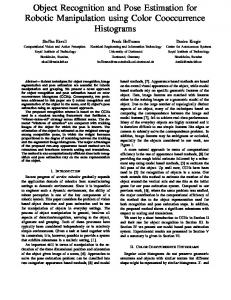
(calibration patterns). Therefore, for this work we focused on the measurement of the errors specifically in 3D pose estimation and tracking. The accuracy of the tracking algorithm was measured in two ways. First, we measured how the tracking algorithm performs the stereo reconstruction and pose estimation when the object is stationary. The second error measurement was regarding the pose estimation for a moving object. 1) Error Measurement for Stationary Target: The goal here was to measure the effects that algorithms such as binarizing, ellipse detection, etc. have in the pose estimation using 3D reconstruction as described in section II-B. Therefore, we ran the tracking algorithm and fixed both object and camera positions while we measured the uncertainties in pixel coordinates of the object features as well as the object pose in the world reference frame. These uncertainties reflect the errors of the algorithms above over a 5-minute sampling period, at 60fps. In Table II we show the experimental results. For this experiment, the pose of the object was calculated at three different relative distances between object and cameras. For each of these distances, four positions of the camera were chosen with respect to the object: top, left, right, and bottom. Each position is about 20cm from the center position. From the table above we notice that the uncertainty (σ ) in the object pose is highly dependent on the uncertainty in the pixel coordinates of the features. Also from the table, the uncertainty in the position of the features seems to be unexpectedly independent of the distance between camera and target object, since at 70cm the error is smaller than at 60 or 80 cm. However, we attribute this behavior to other factors that may also affect the pose estimation, such as the proximity of the object to the vergence point of the cameras, the quality of the tracking for different sizes of the features as perceived in the image, and the illumination conditions (shade and reflectance for different angles/positions). 2) Error Measurement for Moving Target: For this experiment, measuring the error is more difficult than is the case for a stationary target. That is, it is not possible to calculate the ground truth for the object pose if the object is moving. Therefore, instead of measuring the error for a moving target, we fixed the target object and moved the camera (end-effector). The camera/end-effector moved along an arbitrary path, while the pose of the robot endeffector was monitored at each instant when an image was digitized. Fig. 7 depicts plots of the estimated and the actual values for each of the six components of the object pose – x, y, z, yaw, pitch, and roll – as the camera moves along the path. Finally, in Table III, we summarize the statistics of the error in x, y, z, yaw, pitch, and roll. As one may
The X axis is along the vector defined by the cross ¡¡→ ¡¡→ product of the vectors OP1 and OP3 . † The Z axis lies on the plane of the three features and is calculated by the cross product of the X axis and the Y axis. Since P1 , P2 , P3 represent three vectors in the end-effector reference frame, the homogeneous transformation with respect to the object reference frame comes directly from the axes above. Model Features
P3
Z
P2 X
Y O
P1 Object Reference Frame
Fig. 6.
Definition of object reference frame
III. E XPERIMENTAL R ESULTS Before we describe our error measurements, we must present the workspace on which the experiments were carried out. Our workspace consists of a target object placed in front of two stereo cameras mounted on a Kawasaki UX-120 robot end-effector as depicted in Fig. 1. Our system was implemented on a Linux environment running on a Pentium-III 800MHz with 512Mb of system memory. Two externally synchronized Pulnix TMC-7DSP cameras were connected to two Matrox Meteor image grabbers, which can grab pairs of stereo images at 30fps. The system can track all three object features at exactly 60fps (30fps per camera.) In a system such as this one – for assembly of parts on the fly – the various errors in the tracking algorithm ultimately translate into how accurately the tracker positions the end-effector with respect to the target object. These errors originate mainly from: 1) the various calibration procedures such as hand-eye calibration, camera calibration, etc.; 2) the pose estimation using 3D reconstruction of the feature points; and 3) the ability of the system to detect and keep track of the target object. In [6], we have already presented a comprehensive calibration procedure that, for the same workspace, provided an accuracy of 1mm in 3D reconstruction of special objects
3476
TABLE II S TATISTICS OF POSE ESTIMATION UNCERTAINTY FOR A STILL OBJECT; σ :
Distance to object (mm)
σ among all six features (pixel) 0.15 0.29 0.27 0.24 0.22 0.13 0.04 0.30 0.31 0.17 0.30 0.15
Pose with respect to object top left right bottom top left right bottom top left right bottom
600
700
800
Translational uncertainty (mm) σ range 0.495 2.077 0.566 2.918 0.581 2.028 0.280 2.450 0.099 0.301 0.059 1.544 0.076 1.368 0.363 3.102 0.576 5.162 0.160 1.993 0.867 3.694 0.539 3.948
Mean X(mm) Y Z Yaw(degree) Pitch Roll
Yaw
X
0.3
0.2
−0.12
0.1 −0.13
0
Degree
Meter
−0.14
−0.15
Rotational uncertainty (degree) Yaw Pitch Roll σ range σ range σ range 0.033 0.232 0.069 1.824 0.254 0.924 0.035 0.270 0.448 3.005 0.264 1.389 0.032 0.258 0.338 1.947 0.294 1.066 0.077 0.414 0.314 3.360 0.109 1.047 0.077 0.255 0.390 2.629 0.019 0.138 0.038 0.245 0.470 1.287 0.033 0.713 0.008 0.370 0.080 1.294 0.035 0.559 0.058 0.416 0.706 4.084 0.160 0.836 0.052 0.440 0.860 5.053 0.280 2.406 0.026 0.314 0.827 5.414 0.077 0.904 0.102 0.443 0.912 4.994 0.380 1.525 0.076 0.708 0.206 3.586 0.253 2.414
TABLE III M EAN AND STANDARD DEVIATION OF THE ERRORS BETWEEN ACTUAL AND ESTIMATED POSE .
observe, despite the occurrence of a few “off-the-curve” values (large max abs error’s in the table), the translational uncertainty is less than 2.5 mm, while the rotational uncertainty is less than 1.5 degree.
−0.11
STD , RANGE : MAX - MIN
−0.1
-0.094 0.190 -0.703 0.202 -0.162 0.240
Std σ 2.418 1.630 2.210 1.397 0.894 1.497
Max abs error 7.158 5.396 9.298 5.136 3.067 5.540
−0.2
−0.16
−0.3 −0.17
−0.4
−0.18
−0.19
−0.5
0
50
100
150
200
250
300
350
400
−0.6
450
0
50
100
150
200
250
300
350
400
IV. C ONCLUSION AND F UTURE W ORKS
450
Frame number
Frame number
Pitch Y
A real-time stereo tracking algorithm which can estimate the 6-DOF pose of an industrial object with high accuracy was presented. Integrated with the visual servoing system in [1], this tracking algorithm exposes a new frontier in automation of moving assembly lines. In the future, we intend to study the effect of any changes in the vergence angle of the cameras on the target object’s estimated pose. Also, because of the initialization phase, the application of this algorithm is currently constrained to a controlled environment with, for example, distinctive backgrounds, and consistent lighting conditions. While these constraints are not relevant to the tracking phase of the algorithm, these limitations need to be addressed in future work.
0.01
0
−0.01
Degree
Meter
−0.02
−0.03
−0.04
1
−0.05
−0.06
−0.07
−0.08
0 0
50
100
150
200
250
300
350
400
50
100
450
150
200
250
300
350
400
450
300
350
400
450
Frame number
Frame number
Z
Roll
0.9
0.4
0.3
0.88 0.2
0.86 0.1
Degree
Meter
0.84
0.82
0
−0.1
−0.2
0.8 −0.3
0.78
−0.4
−0.5
0.76 0
50
100
150
200
250
Frame number
300
350
400
450
−0.6
0
50
100
150
200
250
Frame number
ACKNOWLEDGEMENT
Fig. 7. Actual (blue plot) and estimated (red plot) values for the X, Y, Z, Yaw, Pitch, and Roll components of the object pose
The authors would like to thank Ford Motor Company for supporting this project.
3477
V. REFERENCES [1] G. N. DeSouza and A. C. Kak. A subsumptive, hierarchical, and distributed vision-based architecture for smart robotics. IEEE Transactions on Robotics and Automation, submitted, 2002. [2] E. Ersu and S. Wienand. Vision system for robot guidance and quality measurement systems in automotive industry. Industrial Robot, 22(6):26–29, 1995. [3] O. D. Faugeras. Three-Dimensional Computer Vision. MIT Press, 1993. [4] J. T. Feddema and O. R. Mitchell. Vision-guided servoing with feature-based trajectory generation. IEEE Transactions on Robotics and Automation, 5(5):691–700, October 1989. [5] C. Harris. Tracking with rigid models. In A. Blake and A. Yuille, editors, Active vision, pages 59–73, Chapter 4, 1992. MIT Press. [6] R. Hirsh, G. N. DeSouza, and A. C. Kak. An iterative approach to the hand-eye and base-world calibration problem. In Proceedings of 2001 IEEE International Conference on Robotics and Automation, volume 1, pages 2171–2176, May 2001. Seoul, Korea. [7] S. Hutchinson, G. D. Hager, and P. I. Corke. A tutorial on visual servo control. IEEE Trans. on Robotics and Automation, 12(5):651–670, Oct. 1996. [8] I. Incorporated. Faceit(tm) face recognition technology. In http://www.identix.com/products/pro faceit.html http://www.cnn.com/2001/US/09/28/rec. airport.facial.screening, 2002. [9] E. Marchand, P. Bouthemy, F. Chaumette, and V. Moreau. Robust real-time visual tracking using a 2d-3d model-based approach. In Proceedings of the 1999 IEEE International Conference on Computer Vision, pages 262–268, Sept. 1999. [10] T. B. Moeslunt and E. Granum. A survey of computer vision-based human motion capture. Computer Vision and Image Understanding, 81(3):231–268, 2001. [11] T. Park and B. Lee. Dynamic tracking line: Feasible tracking region of a robot in conveyor systems. IEEE Transactions on Systems, Man and Cybernetics, 27(6):1022–1030, Dec. 1997. [12] V. I. Pavlovic, R. Sharma, and T. S. Huang. Visual interpretation of hand gestures for human-computer interaction: a review. IEEE Transactions on Pattern Analysis and Machine Intelligence, 19(7):677–695, July 1997. [13] Y. Rui, T. Huang, and S. Chang. Digital image/video library and mpeg-7: standardization and research issues. In Proceedings of ICASSP 1998, 1998.
3478