Realistic and Responsive Network Traffic Generation - UCSD CSE

Realistic and Responsive Network Traffic Generation Kashi Venkatesh Vishwanath and Amin Vahdat University of California, San Diego 9500 Gilman Drive, La Jolla, CA 92093

{kvishwanath,

vahdat}@cs.ucsd.edu

ABSTRACT This paper presents Swing, a closed-loop, network-responsive traffic generator that accurately captures the packet interactions of a range of applications using a simple structural model. Starting from observed traffic at a single point in the network, Swing automatically extracts distributions for user, application, and network behavior. It then generates live traffic corresponding to the underlying models in a network emulation environment running commodity network protocol stacks. We find that the generated traces are statistically similar to the original traces. Further, to the best of our knowledge, we are the first to reproduce burstiness in traffic across a range of timescales using a model applicable to a variety of network settings. An initial sensitivity analysis reveals the importance of capturing and recreating user, application, and network characteristics to accurately reproduce such burstiness. Finally, we explore Swing’s ability to vary user characteristics, application properties, and wide-area network conditions to project traffic characteristics into alternate scenarios.

Categories and Subject Descriptors C.4. [Computer Communication Networks]: Modeling techniques

General Terms Measurement, Design, Experimentation.

Keywords Modeling, Traffic, Generator, Internet, Burstiness, Wavelets, Energy plot, Structural Model

1. INTRODUCTION

The goal of this work is to design a framework capable of generating live network traffic representative of a wide range of both current and future scenarios. Such a framework would be valuable in a variety of settings that includes: capacity planning [27], high-speed router design, queue management studies [23], worm

Permission to make digital or hard copies of all or part of this work for personal or classroom use is granted without fee provided that copies are not made or distributed for profit or commercial advantage and that copies bear this notice and the full citation on the first page. To copy otherwise, to republish, to post on servers or to redistribute to lists, requires prior specific permission and/or a fee. SIGCOMM’06, September 11–15, 2006, Pisa, Italy. Copyright 2006 ACM 1-59593-308-5/06/0009 ...$5.00.

propagation models [37], bandwidth measurement tools [15, 18], network emulation [39, 40] and simulation [30]. We define traffic generation to result in a time-stamped series of packets arriving at and departing from a particular network interface with realistic values for at least the layer 3 (IP) and layer 4 (TCP/UDP) headers. This traffic should accurately reflect arrival rates and variances across a range of time scales, e.g., capturing both average bandwidth and burstiness. Packets should further appropriately map to flow and packet-size distributions, e.g., capturing flow arrival rate, length distributions, etc. We consider two principal challenges to achieving this goal. First, we require an underlying model with simple, semantically meaningful parameters that fully specify the characteristics of a given trace. By semantically meaningful, we mean that it should be straightforward to map high-level application and network conditions to the model. For example, changing network conditions, application mix, or individual application behavior should result in appropriate and realistic effects on the generated traffic. Second, we require techniques to populate the model from existing packet traces to validate its efficacy in capturing trace conditions. That is, traffic based on a model populated from a given packet trace should reproduce the essential characteristics of the original trace. Of course, the model can be populated from a designer’s “first principles” as well, enabling traffic generation corresponding to a variety of scenarios, both real and projected. In this paper, we present the design, implementation, and evaluation of Swing, a traffic generation tool that addresses these challenges. The principal contribution of our work is an understanding of the requirements for matching the burstiness of the packet arrival process of an original trace at a variety of timescales, ranging from fine grained (1 ms) to coarse grained (multiple minutes). Swing matches burstiness for: i) both bytes and packets, ii) both directions (arriving and departing) of a network interface), iii) a variety of individual applications within a trace (e.g., HTTP, P2P, SNMP, NNTP, etc.), and iv) original traces at a range of speeds and taken from a variety of locations. Critical to the success of this effort is our ability to both measure and reproduce in our traffic generation infrastructure the prevailing wide-area network characteristics at the time of the trace. Earlier work shows that it is possible to recreate aggregate trace characteristics (e.g., average bandwidth over a period of minutes) without reproducing wide-area network conditions [36]. We show that reproducing burstiness at a range of timescales (especially sub-RTT) requires recreating network conditions for the transmitting/receiving hosts in the original trace. Of course, extracting wide-area network conditions from a single packet trace is a difficult problem [20, 44]. Thus, a contribution of this work is an understanding of the extent to which existing techniques for

passively measuring wide-area network conditions are sufficient to accurately reproduce the burstiness of a given trace and whether changing assumptions about prevalent network conditions result in correspondingly meaningful changes in resulting traces (e.g., based on halving or doubling the prevalent round trip time). In the Sections that follow we first describe our methodology (§ 2.3) to parameterize (§ 3.1) a given trace and use it to generate (§ 3.3) live traffic and the corresponding packet trace. We first validate (§ 5) Swing’s ability to faithfully reproduce trace characteristics, critically examine (§ 5.3) the sensitivity of generated traces to individual model parameters and finally explore Swing’s ability to project (§ 5.4) traffic characteristics into the future.

2. THE SWING APPROACH 2.1 Requirements

This section describes our goals, assumptions, and approach to packet trace generation. We extract bi-directional characteristics of packets traversing a single network link, our target. Before we describe our approach to trace generation, we present our metrics for success: realism, responsiveness, and maximally random. Packet trace generation is not an end in itself, rather a tool to aid higher-level studies. Thus, the definition of realism for a trace generation mechanism must be considered in the context of its usage. For instance, generating traces for capacity planning likely only requires matching aggregate trace characteristics such as bandwidth over relatively coarse timescales. Trace generation for high-speed router design, queue management policies, bandwidth estimation tools, or flow classification algorithms has much more stringent requirements. We aim to generate realistic traces for a range of usage scenarios and hence our goal is to generate traces that accurately reflect the following characteristics from an original trace: i) packet inter-arrival rate and burstiness across a range of time scales, ii) packet size distributions, iii) flow characteristics including arrival rate and length distributions, and iv) destination IP address and port distributions. In this paper, we present our techniques and results for the first three of these goals. To be responsive, a trace generation tool must flexibly and accurately adjust trace characteristics by allowing the user to change assumptions about the ambient conditions of the original trace, for example the: i) bandwidth capacity of the target link, ii) round trip time distributions of the flows traversing the link, iii) mix of applications sharing a link, e.g., if P2P traffic were to grow to 40% of the traffic on a link or UDP-based voice traffic were to double, and iv) changes in application characteristics, e.g., if average P2P file transfer size grew to 100MB. By maximally random, we mean that a trace generation tool should be able to generate a family of traces constrained only by the target characteristics of the original trace and not the particular pattern of communication in the trace. Thus, multiple traces generated to follow a given set of characteristics should vary (perhaps significantly) across individual connections while still following the appropriate underlying distributions. This requirement eliminates the trivial solution of simply replaying the exact same connections in the exact same order seen in some original trace. While quantifying the extent to which we are successful in generating maximally random graphs is beyond the scope of this paper, this requirement significantly influences our approach to, and architecture for, trace generation.

2.2 Overview

Our hypothesis is that our goals for realistic and responsive packet generation must be informed by accurate models of: i) the users and programs initiating communication across the target link, ii) the hardware, software, and protocols hosting the programs, and iii) the large space of other network links responsible for carrying packets to and from the target link. Without modeling users, it is impossible to study the effects of architectural changes on end users or to capture the effects of changing user behavior (e.g., if user patience for retrieving web content is reduced). Similarly, without an understanding of a wide mix of applications and protocols, it is difficult to understand the effects of evolving application popularity on traffic patterns at a variety of timescales. Finally, the bandwidth, latency, and loss rate of the links upstream and downstream of the target affect packet inter-arrival characteristics and TCP transmission behavior of the end hosts communicating across the target link (see § 5.3). We first describe our methodology for trace generation assuming perfect knowledge of these three system components. In the following sections we describe how to relax this assumption, extracting approximate values for all of these characteristics based solely on a packet trace from some target link. § 5 qualitatively and quantitatively evaluates the extent to which we are able to generate packet traces matching a target link’s observed behavior given our approximations for user, end host, and network characteristics. To generate a packet trace we initiate (non-deterministically) a series of flows in a scalable network emulation environment running commodity operating systems and hardware. Sources and sinks establish TCP and UDP connections across an emulated large-scale network topology with a single link designated as the target. Simply recording the packets and timestamps arriving and exiting this link during a live emulation constitutes our generated trace. The characteristics of individual flows across the target link, e.g., when the flow starts, the pattern of communication back and forth between the source and the sink, is drawn from our models of individual application and user behavior in the original trace. Similarly, we set the characteristics of the wide-area topology, including all the links leading to and from the target link, to match the network characteristics observed in the original trace. We employ ModelNet [39] for our network emulation environment, though our approach is general to a variety of simulation and environment environments. Assuming that we are able to accurately capture and play back user, application, and network characteristics, the resulting packet trace at the target would realistically match the characteristics of the original trace, including average bandwidth and burstiness across a variety of timescales. This same emulation environment allows us to extrapolate to other scenarios not present when the original packet trace was taken. For instance, we could modify the emulated distribution of round trip times or link bandwidths to determine the overall effect on the generated trace. We could similarly modify application characteristics or the application mix to determine effects on the generated trace. A family of randomly generated traces that match essential characteristics of an original trace or empirical distributions for user, application, and network characteristics (that may not have been originally drawn from any existing packet trace) serves a variety of useful purposes. These traces can serve as input to higher level studies, e.g., appropriate queueing policies, flow categorization algorithms, or anomaly detection. Just as interesting however would be employment of the trace generation facility in conjunction with other application studies. For instance, bandwidth or capacity measurement tools may be studied while subject to

a variety of randomly-generated but realistic levels of competing/background traffic at a given link in a simulated or emulated environment. The utility of systems such as application-layer multicast or other overlay protocols could similarly be evaluated while subjecting the applications to realistic cross traffic in emulation testbeds. Most current studies typically: i) assume no competing traffic in an emulated/simulated testbed, ii) subject the application to ad hoc variability in network performance, or iii) deploy their application on network testbeds such as PlanetLab that, while valuable, do not easily enable subjecting an application to a variety of (reproducible) network conditions.

2.3 Structural model

Earlier work [41] shows that realistic traffic generators must use structural models that account for interactions across multiple layers of the protocol stack. We follow the same philosophy and divide our task of finding suitable parameters for Swing’s structural model into four categories: Users: End users determine the communication characteristics of a variety of applications. Important questions include how often users become active, the distribution of remote sites visited, think time between individual requests, etc. Note that certain applications (such as SNMP) may not have a human in the loop, in which case we use this category as a proxy for any regular, even computer-initiated behavior. Sessions: We consider individual session characteristics. For instance, does an activity correspond to downloading multiple images in parallel from the same server, different chunks of the same mp3 file from different servers, etc. An important question concerns the number and target of individual connections within a session. Connections: We also consider the characteristics of connections within a session, such as their destination, the number of request/response pairs within a connection, the size of the request and corresponding response, wait time before generating a response (e.g., corresponding to CPU and I/O overhead at the endpoint), spacing between requests, and transport (e.g., TCP vs. UDP). We characterize individual responses with the packet size distribution, whether it involves constant bit rate communication, etc. Network characteristics: Finally, we characterize the widearea characteristics seen by flows. Specifically, we extract link lossrates, capacities, and latencies for paths connecting each host in the original trace to the target-link. Using these observations, we developed a parameterization of individual application sessions, summarized in Table 1. A set of values for these parameters constitutes an application’s signature. For instance HTTP, P2P, and SMTP will all have different signatures. To successfully reproduce packet traces, we must extract appropriate distributions from the original trace to populate each of the parameters in Table 1. If desired, it is also possible to individually set distribution values for these parameters to extrapolate to a target environment. While we do not claim that our set of parameters is either necessary or sufficient to capture the characteristics of all applications and protocols, in the experiments that we conducted we found each of the parameters to be important for the applications we considered. § 5 quantifies the contribution of a subset of our model parameters to accurately reproduce trace characteristics through an initial sensitivity analysis.

3. ARCHITECTURE

In this section, we present our approach to populating the model outlined above for individual applications, extracting wide-

area characteristics of hosts communicating across the target link, and then generating traces representative of these models.

3.1 Parameterization methodology

We begin with a trace to describe how we extract application characteristics from the target link. While our approach is general to a variety of tracing infrastructures, we focus on tcpdump traces from a given link. The first step in building per-application communication models is assigning packets and flows in a trace to appropriate application classes. Since performing such automatic classification is part of ongoing research [22, 28, 42] and because we do not have access to packet bodies (typically required by existing tools) for most publicly available traces, we take the simple approach of assigning flows to application classes based on destination port numbers. Packets and flows that cannot be unambiguously assigned to an appropriate class are assigned to an “other” application class; we assign aggregate characteristics to this class. While this assumption limits the accuracy of the models extracted for individual applications, it will not impact our ability to faithfully capture aggregate trace characteristics (see § 5). Further, our per-application models will improve as more sophisticated flowclassification techniques become available. After assigning packets to per-application classes, our first task is to group these packets into flows. We use TCP flags (when present) to determine connection start and end times. Next, we use the sequence number and acknowledgment number advancements to calculate the size of data objects flowing in each direction of the connection. Of course, there are many vagaries in determining the start and end of connections in a noisy trace. We use the timestamp of the first SYN packet sent by a host as the connection start time. Unless sufficient information is available in the trace to account for unseen packets for connections established before the trace began, we consider the first packet seen for a connection as the beginning of that connection when we do not see the initial SYN. Similarly, we account for connections terminated by a connection reset (RST) rather than a FIN. Due to space constraints, we omit additional required details such as: out-oforder packets, retransmitted packets, lost packets, and packets with bogus SYN/ACK values. Rather, we adopt strategies employed by earlier efforts faced with similar challenges [32, 35, 20]. Given per-flow, per-application information, we apply a series of rules to extract values for our target parameters. The first step is to generate session information from connection information. We sort the list of all connections corresponding to an application in increasing order of connection establishment times. The first time a connection appears with a given source IP address we designate a session initiation and record the start time. A session consists of one or more RREs (Request-Response-Exchanges). An RRE consists of one or more connections. For instance, 10 parallel connections to download images in a web page constitutes a single RRE. Likewise, the request for the base HTML page and its response will be another RRE. We also initialize the start time of the first connection as the beginning of the first RRE and set the number of connections in this session to 1. Finally, we record the FIN time for the connection. Upon seeing additional connections for an already discerned IP address, we perform one of the following actions. i) If the SYN time of this new connection is within an RREtimeout limit (a configurable parameter), we conclude that the connection belongs to the same RRE (i.e., it is a parallel or simultaneous connection), and update our number of connections parameter. We also update the RREEnd (termination time of all connections) of the RRE as the max of all connection termination times. Finally,

Layer Users RRE Connection Packet Network

Variable in our Parameterization model : Description ClientIP ; numRRE: Number of RREs ; interRRE think time numconn: Number of Connections ; interConn: Time between start of connections numpairs: number of Request/Response exchanges per connection ; Transport: TCP/UDP based on the application ; ServerIP ; RESPonse sizes ; REQuest sizes ; reqthink: User think time between exchanges on a connection packet size: (MTU); bitrate: packet arrival distribution (only for UDP right now) Link Latency ; Delay; Loss rates

Table 1: Structural Model of Traffic. For each new HTTP session, for instance, we pick a randomly generated value (from the corresponding distribution) for each of the variables. First we pick a client and then decide how many RREs to generate along with their interRRE times. For each RRE we decide how many parallel connections (separated by interConn times) to open and to whom (server). Within a connection we decide the total number of request response exchanges along with the request, response sizes and the request think time (reqthink) separating them.

we record the difference in start times of this new connection from the previous connection (interConn) in the same RRE. ii) If the SYN time of this new connection is not within the RREtimeout limit, we declare the termination of the current RRE and mark the beginning of a new RRE. We also calculate the time difference in the max FIN of the previous RRE and the start of this RRE. If that time difference is within the SESStimeout limit (another configurable parameter), we associate the new RRE with an existing session. Otherwise, we conclude that a new session has started. For each connection we also record the request think time as the time difference between a response from the server and the subsequent request from the client. We have analyzed a variety of values for our configurable thresholds such as RREEnd and SESStimeout. While we omit the details for brevity, using RREtimeout = 30sec and SESStimeout = 5min works well for a range of scenarios. In summary, each session consists of a number of RREs, which in turn consist of a number of protocol connections. Given information on individual sessions and their corresponding RREs, we extract a frequency distribution for each to generate empirical cumulative distribution functions (CDF). At this stage, we have the choice of either stopping with the empirical distributions or performing curve-fitting to analytical equations [31]. For this work, we choose the former approach for simplicity and because it accurately represents observed data (for instance, capturing outliers), and leave the derivation and use of analytic distributions to future work.

3.2 Extracting network characteristics

Given models of individual flows crossing a target network link, we next require an understanding of the characteristics of the network links responsible for transmitting data to and from the target link for the hosts communicating across the link. Of course, we can only approximate the dynamically changing bandwidth, latency and loss rate characteristics of all links that carry flows that eventually arrive at our target from a single packet trace. While we developed a number of techniques independently and while it is impossible to determine the extent to which our approach differs from techniques in the literature (where important details may be omitted and source code is often unavailable), we do not necessarily innovate in our ability to passively extract wide-area network conditions from an existing packet trace. Rather, our contribution is to show that it is possible to both capture and replay these network conditions with sufficient fidelity to reproduce essential characteristics of the original trace. § 5 quantifies the extent to which we are successful. Likewise, we assume that the modeled parameters (CDFs) are stationary for the duration of the trace.

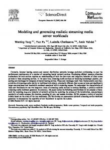
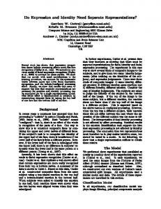
Augmenting our models to account for the changing nature [45] of these (for instance, changing bandwidth) is part of ongoing work. For the traces we consider, non-stationarity has not been a significant obstacle. We extract network characteristics as follows. For each host (unique IP address) communicating across the target link we wish to measure the delays, capacities and loss rates of the set of links connecting the host to the target link as shown in Figure 1. For simplicity, we aggregate all links from a source to the target and the links from the target to the destination into single logical links with aggregate capacity, loss rate, and latency corresponding to the links that make up this aggregate. Thus, in our model we employ four separate logical links (assuming assymetric link characteristics) responsible for carrying traffic to and from the target link for all communicating hosts. For cases where sufficient information is not available—for instance if we do not see ACKs in the reverse direction—we approximate link characteristics for the host as the mean of the observed values for all other hosts on its side of the target link for the same application. Link delays: Consider a flow from a client C initiating a TCP connection to a server S as shown in Figure 1. We use each flow in the underlying trace between these hosts as samples for the four sets of links responsible for carrying traffic between the flow endpoints. We record four quantities for packets arriving at the target link in both directions. First, we record the time difference between a SYN (from C) and the corresponding SYN+ACK (from S) as a sample to estimate the sum of link delays l2 and l3 (Figure 2). Next, we measure the difference between the SYN+ACK and the corresponding ACK packet as samples to estimate the sum of delays l4 and l1 (not shown). We use the difference between a response packet and its corresponding ACK (from C) to estimate the sum of delays l4 and l1 as shown in Figure 3. Finally, we measure the time between a data packet and its corresponding ACK (from S) as further samples for l2 + l3 (not shown). For this analysis, we only consider hosts that have 5 or more sample values in the trace. We use the median (per host) of the sample values to approximate the sum of link delays (l1+l4 or l2+l3). We chose the median because in our current configuration we assign static latency values to the links in our topology and the median should be representative of the time it takes for a packet to reach the target link once it leaves hosts on either end. One assumption behind our work is that flows follow symmetric paths in the forward and reverse direction, allowing us to assign values for l1 and l4 from samples of l1 + l4. Figure 5 for instance shows the two-way delay for hosts on either side of the target link in the Auck trace (§5).

CLIENT C C1,l1,p

1

C4, l4,

p4

SERVER S

TARGET LINK

CLIENT C SERVER S SYN TARGET /ACK LINK SYN

p2 C2, l2, C3, l3,

p3

Figure 1: Approximating wide-area characteristics.

Figure 2: Time difference between a SYN and the corresponding SYN+ACK is an estimate of l2+l3.

Path from C to the target link approximated as a single link with capacity C1, delay l1 and loss rate p1.

HTTP GENERATOR

P2P

SMTP LISTENER

HTTP LISTENER 10 Mbps, 100 ms, 2% loss rate

HTTP LISTENER HTTP GENERATOR

TARGET LINK

FTP GENERATOR

UDP LISTENER

P2P

100 Mbps, 20 ms delay 1% link loss rate 1Gbps, 1ms delay 0.1 % loss rate

SMTP GENERATOR

UDP GENERATOR FTP LISTENER

FTP LISTENER

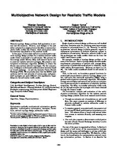
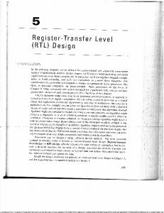
Figure 4: Target link modeled as a Dumb-bell. Link Capacities: We employ the following variant of packetpair techniques to estimate link capacities. We extract consecutive data packets not separated by a corresponding ACK from the other side. The time difference between these packet-pairs gives an estimate [11, 31] of the time for the packets to traverse the bottleneck link from the host to the target link. It is then straightforward to calculate the bottleneck capacity using the formula: LinkCapacity * TimeDifference = PacketSize. With widespread use of delayed ACKs in TCP, half of the packets are sent as packet-pairs. To account for this shortcoming, we sort the packet-pair time separation values in ascending order and ignore the bottom half. Of course, it is known that packet-pair techniques overestimate the bottleneck capacity [11] and moreover doing passive estimation means that we cannot control which packets are actually sent in pairs. To account for this, we use the 50th percentile of the sample values to approximate path capacity from a given host to the target link. For instance, in Figure 3, we can estimate c1 and c3 in this fashion. We assume the incoming link to a host has capacity at least as large as the outgoing link and hence we approximate c4 and c2 to the values c1 and c3 respectively. However, post bottleneck link queueing may reduce packet spacing, inflating our capacity estimates. Likewise, packets sent in pairs might not arrive at the bottleneck in pairs [19]. Improving our capacity estimates based on these recent studies is part of our ongoing work. Loss Rates: We measure loss rates using retransmissions and a simple algorithm based on [5]. The algorithm starts by arranging TCP sequence numbers corresponding to packets of a flow, based on the timestamps. Next, if there is a missing sequence number in the timestamp sequence, it usually means that the corresponding packet was lost en-route to the target link. This is established if the packet (and the corresponding TCP sequence number) is seen at a later time indicating retransmission. Such a missing sequence number is called a “hole” and we count it as a loss event for estimating p1 in Figure 1. Likewise, if there is an out-of-order TCP

CLIENT C

SERVER S

ACK TARGET

LINK

RSP

Figure 3: Time difference between a response packet and the corresponding ACK is an estimate of l4+l1.

packet (retransmission) with no corresponding hole, it is then likely that the packet arrived at the target but was lost en-route to the destination. We use this loss event to estimate p2. p3 and p4 are estimated in a similar manner when we see flows in the opposite direction. Of course the naive algorithm described above needs to be improved to account for spurious timeouts, correlated losses, routing changes, etc., and we refer the reader to [5] for a detailed explanation. Figure 7 shows the loss rate values extracted for both directions of traffic of a trace. We assume that losses experienced by a flow are typically not caused by the traffic we measure directly, i.e., losses on upstream and downstream links are caused by ambient congestion elsewhere in the network and not at some other congestion point shared by multiple hosts from our trace. Using this assumption, we assign distinct loss rates for links connecting each host to the target rather than attempting to account for such shared congestion.

3.3 Generating Swing packet traces

Given application and network models, we are now in position to generate the actual packet trace based on these characteristics. Our strategy is to generate live communication among endpoints exchanging packets across an emulated network topology. We implement custom generators and listeners and pre-configure each to initiate communication according to the application characteristics extracted in the previous step. We also configure the network topology to match the bandwidth, latency, and loss rate characteristics of the original trace as described below. We designate a single link in the configured topology as the target. Our output trace then is simply a tcpdump of all packets traversing the target during the duration of a Swing experiment. We run Swing for 5 minutes more than the duration of the target trace and then ignore the first 5 minutes to focus on steady state characteristics. For each application in the original trace, we generate a list of sessions and session start times according to the distribution of inter-session times measured in the original trace. We then randomly assign individual sessions to generators to seed the corresponding configuration file. For each session, we set values for number of RREs, inter-RRE times, number of connections per RRE, etc., from the distributions measured in the original trace. At startup, each generator reads a configuration file that specifies: i) its IP address, ii) a series of relative time-stamps designating session initiation times (as generated above), iii) the number of RREs for each session, iv) the destination address and communication pattern for each connection within an RRE, and v) the packet size distribution for each connection. For our target scenarios, we typically require thousands of generators, each configured to generate traffic matching the characteristics of a single application/host pair. We create the necessary configuration files for all generators according to our extracted application characteristics. We similarly configure all listeners with their IP

addresses and directives for responding to individual connections, e.g., how long to wait before responding (server think time) and the size of the response. We run the generators and listeners on a cluster of commodity workstations, multiplexing multiple instances on each workstation depending on the requirements of the generated trace. To date, we have generated traces up to approximately 200Mbps. For the experiments in this paper, we use 11 2.8 Ghz Xeon processors running Linux 2.6.10 (Fedora Core 2) with 1GB memory and integrated Gigabit NICs. For example, for a 200Mbps trace, assuming an even split between generators and listeners (five machines each), each generator would be responsible for accurately initiating flows corresponding to 40Mbps on average. Each machine can comfortably handle the average case though there are significant bursts that make it important to “over-provision” the experimental infrastructure. Critical to our methodology is configuring each of the machines to route all packets to a single ModelNet [39] core responsible for emulating the hop-by-hop characteristics of a userspecified wide-area topology. The source code for ModelNet is publicly available and we run version 0.99 on a machine identical to those hosting the generators and listeners. Briefly, ModelNet subjects each packet to the per-hop bandwidth, delay, queueing, and loss characteristics of the target topology. ModelNet operates in real time, meaning that it moves packets from queue to queue in the target topology before forwarding it on to the destination machine (one of the 11 running generators/listeners) assuming that the packet was not dropped because it encountered a full queue or a lossy link. Earlier work [39] validates ModelNet’s accuracy using a single core at traffic rates up to 1Gbps (we can generate higher speed traces in the future by potentially running multiple cores [43]). Simple configuration commands allow us to assign multiple IP addresses (for our experiments, typically hundreds) to each end host.

3.3.1

Creating an emulation topology

The final question revolves around generating the network topology with appropriate capacity, delay, and loss rate values to individual links in the topology. We begin with a single bidirectional link that represents our target link (Figure 4). We assign a bandwidth and latency (propagation delay) to this link based on the derived characteristics of the original traced link. The next step is to add nodes on either side of this target to host generators and listeners. Ideally, we would create one node/edge in our target topology for every unique host in the original trace. However, depending on the size of the trace and the capacity of our emulation environment, it may be necessary to collapse multiple sources from the original trace onto a single IP address/generator in our target topology 1 . For the experiments described in the rest of the paper, we typically collapse up to 10,000 endpoints (depending on the size of the trace) from the original trace onto 1,000 endpoints in our emulation environment. Our mapping process ensures that the generated topology reflects characteristics of the most active hosts. We base the number of generators we assign to each application on the bytes contributed by each application in the original trace. For instance, if 60% of the bytes in the original trace is HTTP, then 60% of our generators (each with a unique IP address) in the emulation topology will be responsible for generating HTTP traffic. 1 Such a collapsing impacts the IP address distribution of flows crossing the target link (i.e., it reduces the number of unique IP addresses in our generated trace relative to the original trace). However, as shown in § 5, this does not affect aggregate trace characteristics, such as bandwidth, packet inter-spacing etc.

We discuss the limitations of this approach in § 6. Next, we assign hosts to both sides of the target link based on the number of bytes flowing in each direction in the original trace for that application. For instance, if there is twice as much HTTP traffic flowing in Figure 4 from left to right as there is from right to left, we would then have twice as many HTTP hosts on the left as on the right in the emulated topology.

3.3.2

Assigning link characteristics to the topology

Given baseline graph interconnectivity consisting of an unbalanced dumb-bell, we next assign bandwidth and latency values to these links. We proceed with the distributions measured in the original trace (§ 3.2) and further weigh these distributions with the amount of traffic sent across those links in the original trace. Thus, if a particular HTTP source in the original trace were responsible for transmitting 20% of the total HTTP bytes using a logical link with 400 kbps of bandwidth and 50 ms of latency, a randomly chosen 20% of the links (corresponding to HTTP generators) in our target topology would be assigned bandwidth/latency values accordingly. We also assign per-link MTUs to each link based on distributions from the original trace. The topology we have at the end of this stage is not one that accurately represents the total number of hosts with the same distribution of wide-area characteristics as in the original trace, but one that is biased towards hosts that generate the most traffic in the original trace. One alternative is to assign sessions to generators based on the network characteristics of the sources in the original trace. We have implemented this strategy as well and it produces better results with respect to matching trace characteristics, but we found that it did not offer sufficient randomness in our generated traces, i.e., the resulting traces too closely matched the characteristics of the original trace making it less interesting from the perspective of exploring a space or extrapolating to alternative scenarios.

4. VALIDATION

We now describe our approach for extracting and validating our parameter values for our model from a number of available packet traces. In particular, we focus on Mawi [26] traces, a transPacific line (18Mbps Committed Access Rate on a 100Mbps link), CAIDA [6] traces from a high-speed OC-48 MFN (Metropolitan Fibre Network) Backbone 1 link (San Jose to Seattle) as well as OC3c ATM link traces from the University of Auckland, New Zealand [2]. These traces come from different geographical locations and demonstrate variation in application mix and individual application characteristics (Table 2). For each trace 2 , we first extract distributions of user, network and application using the methodology outlined in § 3. Next we generate traffic using Swing and during the live emulation record each packet that traverses our target link. From the generated Swing-trace we re-extract parameter values and compare them to the original values in Table 3. Specifically, we compare: i) application breakdown, ii) aggregate bandwidth consumption, iii) packet and byte arrival burstiness, iv) per-application bandwidth consumption, and v) distributions for our model’s parameter values. To compare distributions we use various techniques ranging from visual tests to comparing the median values and Inter-Quartile 3 ranges. To determine whether we capture the burstiness characteristics of the original trace, we employ wavelet-based multi-resolution 2 3

UDP traffic (∼ 10% by bytes) was filtered out. IQR is the difference in the 75th and 25th percentile values.

Table 2: Comparing aggregate bandwidth (Mbps) and packets per second (pps) (Trace/Swing) for Auck, Mawi and CAIDA traces. Trace ↓ Auck Mawi Mawi2 CAIDA

Length Secs 599 899 299 300

TOTAL Mbps pps 5.53 979 17.79 2229 21.96 2907 184.17 22786

Date 2001-06-11 2004-09-23 2004-03-18 2003-04-24

Application 1 - HTTP Mbps pps 3.33 / 3.24 591 / 509 9.90 / 9.04 1209 / 1101 13.88 / 12.24 1779 / 1567 134.93 / 127.56 17404 / 14625

Name SQUID TCPOTHER TCPOTHER KAZAA

Application 2 Mbps 0.55 / 0.55 5.58 / 4.96 7.51 / 7.63 49.24 / 45.97

pps 58 / 57 720 / 609 972 / 890 5382 / 4523

Table 3: Median and IQR parameter values (Trace/Swing) for Auck, Mawi and CAIDA traces. Model Parameters→ (Trace)Application(Statistic)↓ (Auck) HTTP (Median) (Auck) HTTP (IQR) (Auck) SQUID (Median) (Auck) SQUID (IQR) (Mawi) HTTP (Median) (Mawi) HTTP (IQR) (Mawi) TCPOTHER (Median) (Mawi) TCPOTHER (IQR) (CAIDA) HTTP (Median) (CAIDA) HTTP (IQR) (CAIDA) KAZAA (Median) (CAIDA) KAZAA (IQR)

REQ (Bytes) 420 / 421 201 / 203 535 / 536 178 / 181 415 / 414 406 / 408 36 / 36 1014 / 642 341 / 341 446 / 464 57 / 57 319 / 316

RSP (Bytes) 747 / 735 3371 / 3357 1649 / 1523 5224 / 5225 462 / 438 2956 / 2947 68 / 80 516 / 755 361 / 355 6705 / 6649 100 / 96 317 / 324

numconn

analysis (MRA) [1, 17, 21] to compare byte and packet-arrival rates at varying time scales. Intuitively, wavelet scaling plots, or energy plots, show the variance (burstiness) in the traffic arrival process at different timescales. It enables visual inspection of the complex structure in traffic processes. For example, consider the top pair of curves in Figure 8. The x-axis represents increasing time scales (on a log scale) beginning at 1 ms and the y-axis is the Energy of the traffic at a given time scale. A sharp dip in the curve, for instance, one that happens at time scale of 9 (256ms) suggests a strong periodicity (and hence lower variance and Energy) around that time scale. The presence of a dip at the time scale of the dominant RTT of flows is well understood [12, 21, 41] and results from the selfclocking nature of TCP. Likewise, if all flows arriving at a target link are bottle-necked upstream at a link whose capacity is 10Mbps, then we would expect a dip at 1.2ms (the time to transmit a 1500 byte packet across a 10Mbps link). For more detailed analysis and interpretation, we refer the reader to [1, 12]. For our purposes, if the energy plot for a generated trace closely matches the energy plot for the original trace, then we may conclude that the burstiness of the packet or byte arrival process matches at a variety of timescales for the two traces. Such matching is important if the generated traces are to be successfully employed for scenarios sensitive to burstiness, e.g., high-speed router design, active queue management, or flow classification. Matching the energy plot of a given plot at both fine- (sub-RTT) and coarsetimescales has proven difficult. To the best of our knowledge, our work is the first to show such a match across a range of timescales.

5. APPLICATION STUDIES

Given our general validation approach, we now present the results of case studies for: i) capturing the fine-grained behavior of individual application classes in our packet traces, ii) validating

1/1 1/1 2/2 6/6 1/1 0/0 1/1 0/0 1/1 1/1 1/1 0/0

interconn (Secs) 0.4 / 0.4 1.0 / 0.9 1.0 / 1.0 2.7 / 2.2 0.7 / 0.7 2.2 / 2.0 1.5 / 1.5 4.9 / 3.3 0.5 / 0.6 1.8 / 1.8 1.3 / 1.4 2.7 / 2.6

numpairs

numrre

1/1 0/0 1/1 2/2 1/1 0/0 1/1 5/5 1/1 0/0 1/1 0/0

1/1 0/1 1/1 1/1 1/1 0/0 1/1 0/0 1/1 0/1 1/1 0/0

interRRE (Secs) 10.9 / 10.5 8.8 / 8.4 8.6 / 7.7 7.6 / 4.1 10.6 / 10.2 9.4 / 8.4 10.7 / 11.4 9.5 / 10.3 10.2 / 10.5 8.9 / 9.0 12.0 / 16.2 14.9 / 12.2

reqthink (Secs) 0.1 / 0.1 0.8 / 0.8 0.6 / 0.6 1.4 / 1.4 0.2 / 0.2 2.0 / 1.9 0.1 / 0.1 0.3 / 0.3 0.1 / 0.0 0.6 / 0.5 0.2 / 0.1 0.6 / 0.5

macro properties of our generated traces, and iii) matching burstiness of traffic across a range of time granularities.

5.1 Distribution parameters

We first measure Swing’s ability to accurately capture the distributions for the structural properties of users and applications. We present results for three representative applications taken from our three traces: KAZAA from CAIDA, SQUID from Auck, and HTTP from Mawi. Importantly, our model is generic to each of these application classes and requires no manual configuration for the various traces/applications. Results for other application classes/trace combinations are similar. Table 3 compares the distribution of our parameters relative to the original trace (Trace/Swing), with the median values and IQR. Matching IQR values and the median indicates similar distributions for both the extracted and generated values. While the required level of accuracy is application-dependent, based on these results we are satisfied with our ability to reproduce application and user characteristics. We have found that model parameters that attempt to reproduce human/machine think time are the most difficult to accurately extract and reproduce. For instance, the IQR of interconn times for Auck/SQUID differs by 500ms. However, our sensitivity experiments (§ 5.3) reveal that it is important to consider these characteristics to reproduce trace properties and that our approximations appear sufficient based on the quality of the generated traces. On the other hand, we achieve near perfect accuracy for more mechanistic model parameters such as request and response size (see Table 3). Given validation of our application and user models, we next consider wide-area network conditions. Figure 5 shows the extracted values of the two-way latencies of hosts on either side of the target link in the Auck trace. More than 75% of the hosts see

AuckDir0 SwingDir0 AuckDir1 SwingDir1

0.2 0

0.6

0

26 24

Smallest time scale = 1 msec

25

AuckDir0 AuckDir1 SwingDir0 SwingDir1

22 20 18 16 0

5

10 Time Scale j

15

Figure 8: HTTP/Auck Energy plot (bytes).

0

50 100 150 Link Capacities of hosts (mbps)

20

0.4 0.2

5

10 Time Scale j

15

Figure 9: SQUID/Auck Energy plot (bytes).

Figure 8 compares the wavelet scaling plots for byte arrivals for HTTP/Auck and corresponding Swing traces. In both plots, the top pair of curves corresponds to the scaling plots for one traffic direction (labeled 0) and the bottom curves are for the opposite direction (labeled 1). A common dip in the top curve corresponds

Auck Swing

0

0

5 10 15 Loss rate of links (percentage)

20

Figure 7: Loss rates for feeding links

5

AuckDir0 AuckDir1 SwingDir0 SwingDir1

a delay of greater than 200ms on one side of the link (Direction 1) matching our expectation for a cross-continental link. Figure 6 compares Auck’s link capacities for the path connecting the hosts to the target-link. While in one direction the capacities range from 1 − 100Mbps, hosts appear to be bottlenecked upstream at approximately 3.5Mbps in the other direction. These values match our understanding of typical host characteristics on either side of the Auck link (we had similarly good results for Mawi and CAIDA). Finally, Figure 7 presents the loss rate for the trace. For validation, we also plot the extracted values for delay, capacity, and loss rate for our Swing-generated traces. We obtain good matches in all cases. The discrepancy in loss rate behavior results from the difficulty of disambiguating between losses, retransmissions, and multi-path routing in a noisy packet trace. Finally, Table 2 presents aggregate per-application characteristics of Swing-generated traces compared to the original Auck, Mawi, and CAIDA traces. In all cases, we are satisfied with our ability to reproduce aggregate trace characteristics, especially considering that we are performing no manual tuning on a per-trace or per-application basis. While we focus on our ability to reproduce per-application characteristics in this paper, our results are typically better when reproducing aggregate trace characteristics because of the availability of more information and less discretization error.

5.2 Wavelet based analysis

0.6

Smallest time scale = 1 msec

15

10 0

0.8

200

Figure 6: Upstream and downstream Capacities.

log2(Energy(j))

28

AuckDir0 SwingDir0 AuckDir1 SwingDir1

0.2

0 200 400 600 800 Delay from host to the target link (msec)

Figure 5: Two-way delay for hosts.

log2(Energy(j))

0.8

0.4

Comparing CDFs of loss rates

1

log2(Energy(j))

0.6

Cumulative fraction

Cumulative fraction

0.8

0.4

Comparing CDFs of link capacities

1

Cumulative fraction

Comparing CDFs of host delays

1

0

Smallest time scale = 1 msec AuckDir0 AuckDir1 SwingDir0 SwingDir1

−5

−10 0

5

10 Time Scale j

15

Figure 10: SQUID/Auck Energy plot (packets).

to the dominant RTT of 200ms (scale 9) as shown in Figure 5. Likewise, the common dip seen for the bottom pair at a scale of 3 (8ms) corresponds to the bottleneck upstream capacity of 3.5Mbps (see Figure 6). Figure 9 compares the scaling plots for byte arrivals for SQUID for the same trace. The relatively flat structure in Direction 1 relative to the HTTP plot results because most of the data flows in Direction 0. The significant difference in SQUID’s behavior relative to HTTP shows the importance of capturing individual application characteristics, especially if using Swing to extrapolate to other network settings, e.g., considering trace behavior in the case when SQUID becomes the dominant application. Figure 10 shows the corresponding plot for packet arrivals. The close match confirms our ability to reproduce burstiness at the granularity of both bytes and packets. Figure 11 shows the scaling plot for HTTP byte arrivals in the Mawi trace. The plot differs significantly from the corresponding Auck plot (see Figure 8) but Swing can accurately reproduce it without manual tuning. Consider another trace from the Mawi repository taken six months earlier as shown in Figure 12. Application burstiness changes over time in this trace and Swing accurately captures this evolving behavior. Finally, Figure 13 shows the energy plot for both directions of HTTP traffic in the CAIDA trace as validation of our ability to generalize to a higher-bandwidth trace as well as to a trace taken from a fundamentally different network location. To the best of our knowledge, we are the first to reproduce observed burstiness in generated traces across a range of time scales. While our relatively simple model cannot capture all relevant trace conditions (such as the number of intermediate hops to the target link), an important contribution of this work demonstrates

26 log2(Energy(j))

25

20 0

5

10 Time Scale j

LatencyCapacityLossRates LatencyCapacities LinkLatencies NoNetwork Mawi

5 10 Time Scale j

30

Smallest time scale = 1 msec CAIDADir0 CAIDADir1 SwingDir0 SwingDir1

25

25

HTTP NoInterrreHTTP SQUID NoInterconnSQUID

5

10 Time Scale j

15

Figure 14: Energy plot sensitivity to network characteristics.

0

15

24

Smallest time scale = 1 msec SwingDir0AvgOf10Runs AuckDir0 SwingDir1AvgOf10Runs AuckDir1

22 20 18 16

5

10 Time Scale j

15

Figure 15: Energy plot sensitivity to interconn, interRRE parameters.

that capturing and reproducing a relatively simple set of trace conditions is sufficient to capture burstiness, at least for the traces we considered. Earlier work [12] shows that global scaling (at time scales beyond the dominant RTT) can be captured by modeling, for instance, response sizes as a heavy-tailed distribution. Our work on the other hand, shows how to extract appropriate distributions from the underlying trace (rather than assuming particular distributions for individual parameters), reproduces burstiness at a variety of time scales (including those smaller than the dominant RTT), and considers both the bytes and packet arrival processes for traffic in two directions.

5.3 Sensitivity

28 26

20

5 10 Time Scale j

Figure 13: HTTP/CAIDA Energy plot (bytes).

Smallest time scale = 1 msec

15

20

20 0

15

Figure 12: HTTP/Mawi2 Energy plot (bytes).

log2(Energy(j))

log2(Energy(j))

20

30

25

0

22

16 0

15

Smallest time scale = 1 msec

30

35

18

Figure 11: HTTP/Mawi Energy plot (bytes). 35

24

Smallest time scale = 1 msec MawiDir0 MawiDir1 SwingDir0 SwingDir1

log2(Energy(j))

log2(Energy(j))

30

28

log2(Energy(j))

Smallest time scale = 1 msec MawiDir0 MawiDir1 SwingDir0 SwingDir1

One question is whether our model parameters are necessary and sufficient to reproduce trace characteristics. Similarly, it would be interesting to quantify the relative importance of individual parameters under different settings. While a detailed analysis is beyond the scope of this paper, we have investigated trace sensitivity to our parameters and have found that all aspects of our model do indeed influence resulting accuracy to varying extents. We present a subset of our findings here. We start with the importance of capturing and reproducing wide-area network conditions as it appears to be the biggest contributor to burstiness in the original trace. Consider the case where we omit emulating wide-area network conditions and simply play back modeled user and application characteristics across an unconstrained network (switched Gigabit Ethernet). While we roughly maintain aggregate trace characteristics such as bandwidth (not shown), Figure 14 shows that we lose the rich structure present at sub-RTT scales and the overall burstiness characteristics. This result shows that two generated traces with the same average-case

0

5

10 Time Scale j

15

Figure 16: Cross-run Energy plot variability.

behavior can have vastly different structure. Hence, it is important to consider network conditions to reproduce the structure in an original trace. This figure also shows that capturing any single aspect of wide-area network conditions is likely insufficient to reproduce trace characteristics. For instance, only reproducing link latencies (with unconstrained capacity and no loss rate) improves the shape of the plot relative to an unconstrained network but remains far from the original trace characteristics. Likewise, having both latency and capacity is also insufficient though progressively better. Accurate network modeling alone is insufficient to reproduce burstiness. As one example, the top two curves in Figure 15 show the degradation when we omit interRRE from our model for HTTP/Auck. Similarly, the bottom pair of curves show the increase in burstiness at large time scales when we omit interconn for SQUID/Auck. As in § 2, one of our goals is to generate a family of traces starting from a given trace using indepedent model and parameters. While this approach allows us to introduce more variability in Swing-generated traces, it is important to consider the resulting deviation from the original trace. To address this question we perform the following experiment. We start with the Auck trace and vary the initial random seed to our traffic generator and generate 10 Swing traces. Figure 16 shows the variability across the different runs. For Swing curves, we plot average values across the 10 runs for each time scale and show the standard deviation using error bars. While the average curves closely follow Auck, at large time scales we see a few examples where the energy plot does not completely overlap with the baseline. While it is feasible to reduce variability, overall we prefer the ability to explore the range of possible behavior starting with an original trace.

5.4 Responsiveness

Smallest time scale = 1 msec

log2(Energy(j))

28

Swing RSPDouble LatencyDouble

26 24 22 20 0

5

10 Time Scale j

26 24

SwingWithSQUID*20 AuckBaseline SwingBaseline AuckOnlySQUID

22 20 18 16 0

5

10 Time Scale j

15

Figure 18: Energy plot responsiveness to varying application mix (Auck).

Smallest time scale = 1 msec 30

28 log2(Energy(j))

We now explore Swing’s ability to project traffic into alternate scenarios. Figure 17 shows the effect of doubling the link latencies (all other model parameters remain unchanged) for HTTP/Mawi. Once again, while aggregate trace characteristics are roughly maintained (8.17mbps vs. 9mbps), burstiness can vary significantly. Overall, we find that relatively accurate estimates of network conditions (at least within a factor of two) are required to capture burstiness and that, encouragingly, changing estimates for network conditions match expectations for the resulting energy plot. For instance, doubling the RTT moves the significant dip to the right by one unit as the X-axis is on a log2 scale. We also consider the

15

Figure 17: Energy plot responsiveness to doubling response size and link latency (Mawi). effects of doubling request and response sizes for the same trace. Once again, the energy plot shows the expected effect: the relative shape of the curve remains the same, but with significantly more energy at all time scales. The average bandwidth increases from 9mbps to 19mbps. Finally, we explore Swing’s ability to project to alternate application mixes during traffic generation. For the Auck trace (Table 2), we increase the number of SQUID sessions by a factor of 20 while leaving all other model parameters (for different applications and network conditions) identical. The average bandwidth of the trace increased to 15mbps. Earlier figures 8 and 9 highlighted the difference in burstiness characteristics of the two applications. SQUID has a much more pronounced dip at time scale 9 and the curve in smaller time scales is more convex in shape. The energy plot of the overall trace is a function of the burstiness of individual applications and hence increasing the percentage of SQUID should make the overall energy plot resemble SQUID. Figure 18 shows the curves that verify this hypothesis. For comparison we also show the energy plot corresponding to SQUID in the original trace.

6. LIMITATIONS AND FUTURE WORK

In addition to the discussion in the body of the paper, we identify a number of additional limitations with methodology in this section. First, we model application behavior based on the information we can glean from the available packet traces containing only packet headers. A number of efforts have studied application behavior by tracing full application-level information for peer-to-peer [14], multimedia [38], and HTTP [3] workloads. In ongoing work, we aim to show that our model can be populated from such application-level traces and workload generators. Our initial results are encouraging. Swing’s accuracy will be limited by the accuracy of the models it extracts for user, application, and network behavior.

The quality of our traces also impacts our results. For instance, we have found inter-packet timings in pcap traces that should not be possible based on the measured link’s capacity. Pervasive routing asymmetry also means that bi-directional model extraction can introduce errors in some cases. Finally, using homogeneous protocol stacks on end hosts limit our ability to reproduce the mix of network stacks (e.g., TCP flavors) seen across an original trace. Because we are generating traffic for a dumbbell topology and we focus on producing accurate packet traces in terms of bandwidth and burstiness we only focus on a subset of our initial parameters. In particular we do not currently model the distribution of requests and responses among particular clients and servers and we do not model server think time. We split the total number of hosts in the emulation topology weighed by the number of bytes transmitted per-application in the original trace. One problem with this approach is that we lose the spatial locality of the same host simultaneously engaging in, e.g., HTTP, P2P and SMTP sessions. Finally, in this paper we only consider TCP applications. Our implementation does support UDP but we leave a detailed analysis of our techniques and accuracy to future work. In this work, we focus on generating realistic traces for a single network link. For a variety of studies, it may be valuable to simultaneously generate accurate communication characteristics across multiple links in a large topology. We consider this to be an interesting and challenging avenue for future research though it will likely require access to simultaneous packet traces at multiple vantage points to accurately populate some extended version of our proposed model.

7. RELATED WORK

Our work benefits from related efforts in a variety of disciplines. We discuss a number of these areas below. Application-specific workload generation: There have been many attempts to design application-specific workload generators. Examples include Surge [3], which follows empirically-derived models for web traffic [25] and models of TELNET, SMTP, NNTP and FTP [31]. Cao et.al [7] perform source-level modeling of HTTP. However, they attempt to parameterize the round-trip times seen by the client rather than capture it empirically. Relative to these efforts, Swing attempts to capture the packet communication patterns of a variety of applications (rather than individual applications) communicating across wide-area networks. Applicationspecific workload generators are agnostic to particular network bandwidths and latencies, TCP particularities, etc. Although recent efforts characterize P2P workloads at the packet [14] and flow

level [34] we are not aware of any real workload generator for such systems. Synthetic traffic trace generation: One way to study statistical properties of applications and users is through packet traces from existing wide-area links, such as those available from CAIDA [6] and NLANR [29]. However, these traces are based on past measurements, making it difficult to extrapolate to other workload and topology scenarios. RAMP [8] generates high bandwidth traces using a simulation environment involving source-level models for HTTP and FTP only. We, on the other hand advocate a single parameterization model with different parameters (distributions) for different applications. Rupp et. al [33] introduce a packet trace manipulation framework for testbeds. They present a set of rules to manipulate a given network trace, for instance, stretch the duration of existing flows, add new flows, change packet size distributions, etc. Our approach is complementary as we focus on generating the traces using a first-principles approach by constructing real packetexchanging sources and sinks. Structural model: The importance of structural models is well documented [13, 41], but a generic structural model for Internet applications does not exist to date. Netspec [24] builds source models to generate traffic for Telnet, FTP, voice, video and WWW but the authors do not show whether the generated traffic is representative of real traffic. There is also a source model for HTTP [7]. However, it consists of both application-dependent and network-dependent parameters (like RTT), making it difficult to interpret the results and apply them to different scenarios. There are a number of other available traffic generators [10], however, none attempt to capture realistic Internet communication patterns, leaving parameterization of the generator to users. To the best of our knowledge, we present the first unified framework for structural modeling of a mix of applications. Capturing communication characteristics: There have been attempts to classify applications based on their communication patterns [22, 28, 35, 42]. Generating traffic based on clusters of applications grouped according to an underlying model is part of our ongoing effort. Harpoon [36] is perhaps most closely related to our effort. However, there are key differences in the goals of the two projects, with corresponding differences in design choices and system capabilities. Harpoon models background traffic starting with measured distributions of flow behavior on a target link. Relative to their effort, we consider the characteristics of individual applications enabling us to vary the mix of, for instance, HTTP versus P2P traffic in projected future settings. More importantly, Harpoon is designed to match distributions from the underlying trace at a coarse granularity (minutes) and thus does not either extract or playback network characteristics. Swing, on the other hand, extracts distributions for the wide-area characteristics of flows that cross a particular link, enabling us to reproduce burstiness of the packet-arrival process at sub-RTT time scales. This further allows us to predict the effects, at least roughly, on a packet trace of changing network conditions. Relative to recent work investigating the causes for sub-RTT burstiness [21], we focus on extracting the necessary characteristics from existing traces to reproduce such burstiness in live packet traces. As part of future work, we hope to corroborate their findings regarding the causes of sub-RTT burstiness. Felix et. al [16] generate realistic TCP workloads using a one-to-one mapping of connections from the original trace to the test environment. Our effort differs from theirs in a number of ways. We develop a session model on top of their connection model and this is crucial since the termination time of previous

connections determine the start duration of future connections for a user/session, thereby making any static connection replay model essentially unresponsive to changes in the underlying model. As described earlier, we also advocate a common parameterization model for various application classes instead of grouping them all under one class. Passive estimation of wide-area characteristics: Our effort builds upon existing work on estimating wide-area network characteristics without active probing. Jaiswal et. al [20] use passive measurement to infer round trip times by looking at traffic flowing across a single link. Our methodology for estimating RTTs is closely related to this effort, though we extend it to build distinct distributions for the sender- versus receiver-side. Our approach to measuring RTT distributions is more general than the popular approach of measuring a single RTT distribution and dividing it by two to set latencies on each side of the target link [9]. Such techniques assume that the target link is close to the border router of an organization, an assumption that is clearly not general to arbitrary traces (including Mawi). Our techniques for estimating link capacity measure the mean dispersion of packet pairs sent from the sender to the target link, as in [11, 19]. Finally, we resolve ambiguities in loss rate estimates using techniques similar to [5]. Our approach to measuring RTT and loss rates is also similar to T-RAT [44]. However, our goals are different: while T-RAT focuses on analyzing the cause for slowdowns on a per-flow basis, we are interested in determining the distribution of network characteristics across time for individual hosts. In [4] the authors profile various delay components in Web transactions by tracing TCP packets exchanged between clients and servers. This work assumes the presence of traces at both the client and server side and focuses on a single application. For our work, we utilize a single trace at an arbitrary point in the network and extract information on a variety of applications. Further, while we focus on generating realistic and responsive packet traces based on the measured application, network, and user behavior at a single point in the network, their effort focuses on root-cause analysis— determining the largest bottleneck to end-to-end performance in a particular system deployment.

8. CONCLUSIONS

In this paper, we develop a comprehensive framework for generating realistic packet traces. We argue that capturing and reproducing essential characteristics of a packet trace requires a model for user, application, and network behavior. We then present one such model and demonstrate how it can be populated using existing packet header traces. Our tool, Swing, uses these models to generate live packet traces by matching user and application characteristics on commodity operating systems subject to the communication characteristics of an appropriately configured emulated network. We show that our generated traces match both aggregate characteristics and burstiness in the byte and packet arrival process across a variety of timescales when compared to the original trace. Further, we show initial results suggesting that users can modify subsets of our semantically meaningful model to extrapolate to alternate user, application, and network conditions. Overall, we hope that Swing will enable quantifying the impact on traffic characteristics of: i) changing network conditions, such as increasing capacities or decreasing round trip times, ii) changing application mix, for instance, determining the effects of increased peer-to-peer application activity, and iii) changing user behavior, for example, determining the effects of users retrieving video rather than audio content. Similarly, Swingwill enable the evaluation of a variety of higher-level application studies, such as

bandwidth/capacity estimation tools and dynamically reconfiguring overlays, subject to realistic levels of background traffic and network variability.

ACKNOWLEDGEMENTS

We would like to thank Vern Paxson for his insightful and detailed comments in the early days of this work, and Daryl Veitch for making available the code for creating wavelet scaling plots. Credits are due to the anonymous reviewers who made valuable suggestions to improve the work, and finally to thank NLANR, WIDE, and CAIDA, who have made this research possible by allowing access to a large repository of network traces.

9. REFERENCES [1] A BRY, P., AND V EITCH , D. Wavelet analysis of long-range-dependent traffic. IEEE Transactions on Information Theory 44, 1 (1998), 2–15. [2] Auckland-VI trace archive, University of Auckland, New Zealand. http://pma.nlanr.net/Traces/long/auck6.html. [3] BARFORD , P., AND C ROVELLA , M. Generating representative web workloads for network and server performance evaluation. In MMCS (1998), pp. 151–160. [4] BARFORD , P., AND C ROVELLA , M. Critical path analysis of TCP transactions. In ACM SIGCOMM (2000). [5] B ENKO , P., AND V ERES , A. A passive method for estimating end-to-end tcp packet loss. In IEEE Globecom (2002). [6] CAIDA. http://www.caida.org. [7] C AO , J., C LEVELAND , W., G AO , Y., J EFFAY, K., S MITH , F. D., AND W EIGLE , M. Stochastic models for generating synthetic http source traffic. In IEEE INFOCOMM (2004). [8] CHAN L AN , K., AND H EIDEMANN , J. A tool for rapid model parameterization and its applications. In MoMeTools Workshop (2003). [9] C HENG , Y.-C., H OELZLE , U., C ARDWELL , N., S AVAGE , S., AND VOELKER , G. M. Monkey see, monkey do: A tool for tcp tracing and replaying. In USENIX Technical Conference (2004). [10] DANZIG , P. B., AND JAMIN , S. tcplib: A library of TCP/IP traffic characteristics. USC Networking and Distributed Systems Laboratory TR CS-SYS-91-01 (October, 1991). [11] D OVROLIS , C., R AMANATHAN , P., AND M OORE , D. Packet dispersion techniques and capacity estimation. In IEEE/ACM Transactions in Networking, Dec (2004). [12] F ELDMANN , A., G ILBERT, A. C., H UANG , P., AND W ILLINGER , W. Dynamics of IP traffic: A study of the role of variability and the impact of control. In ACM SIGCOMM (1999). [13] F LOYD , S., AND PAXSON , V. Difficulties in simulating the internet. In IEEE/ACM Transactions on Networking (2001). [14] G UMMADI , K. P., D UNN , R. J., S AROIU , S., G RIBBLE , S. D., L EVY, H. M., AND Z AHORJAN , J. Measurement, modeling, and analysis of a peer-to-peer file-sharing workload. In Symposium on Operating Sytems Principles (SOSP) (2003). [15] H ARFOUSH , K., B ESTAVROS , A., AND B YERS , J. Measuring bottleneck bandwidth of targeted path. In IEEE INFOCOM (2003). [16] H ERNANDEZ -C AMPOS , F., S MITH , F. D., AND J EFFAY, K. Generating realistic tcp workloads. In CMG2004 Conference (2004). [17] H UANG , P., F ELDMANN , A., AND W ILLINGER , W. A non-intrusive, wavelet-based approach to detecting network performance problems. In Internet Measurement Workshop (2001). [18] JAIN , M., AND D OVROLIS , C. End-to-end available bandwidth: Measurement methodology, dynamics, and relation with tcp throughput. In ACM SIGCOMM (2002). [19] JAIN , M., AND D OVROLIS , C. Ten fallacies and pitfalls in end-to-end available bandwidth estimation. In Internet Measurement Conference (2004). [20] JAISWAL , S., I ANNACONE , G., D IOT, C., K UROSE , J., AND T OWSLEY, D. Inferring tcp connection characteristics through passive measurements. In IEEE INFOCOM (2004). [21] J IANG , H., AND D OVROLIS , C. Why is the internet traffic bursty in short (sub-rtt) time scales? In SIGMETRICS (2005).

[22] K ARAGIANNIS , T., PAPAGIANNAKI , K., AND FALOUTSOS , M. Blinc: Multilevel traffic classification in the dark. In ACM SIGCOMM (2005). [23] L E , L., A IKAT, J., J EFFAY, K., AND S MITH , F. D. The Effects of Active Queue Management on Web Performance. In ACM SIGCOMM (2003). [24] L EE , B. O., F ROST, V. S., AND J ONKMAN , R. Netspec 3.0 source models for telnet, ftp , voice, video and WWW traffic. In Technical Report ITTC-TR-10980-19, University of Kansas (1997). [25] M AH , B. A. An empirical model of HTTP network traffic. In IEEE INFOCOM (2) (1997). [26] Mawi working group traffic archive. http://tracer.csl.sony.co.jp/mawi/. [27] M EDINA , A., TAFT, N., S ALAMATIAN , K., B HATTACHARYYA , S., AND D IOT, C. Traffic Matrix Estimation: Existing Techniques and New Directions. In ACM SIGCOMM (2002). [28] M OORE , A., AND Z UEV, D. Internet traffic classification using bayesian analysis techniques. In ACM SIGMETRICS (2005). [29] The national laboratory for applied network research (nlanr ) http://www.nlanr.net. [30] The network simulator ns-2. http://www.isi.edu/nsnam/ns. [31] PAXSON , V. Empirically derived analytic models of wide-area TCP coections. IEEE/ACM Transactions on Networking 2, 4 (1994), 316–336. [32] PAXSON , V. End-to-end internet packet dynamics. In IEEE/ACM Transactions on Networking, Vol.7, No. 3 (June, 1999), pp. 277–292. [33] RUPP, A., D REGER , H., F ELDMANN , A., AND S OMMER , R. Packet trace manipulation framework for test labs. In Internet Measurement Conference (2004). [34] S EN , S., AND WANG , J. Analyzing peer-to-peer traffic across large networks. In ACM SIGCOMM Internet measurement workshop (2002). [35] S MITH , F. D., H ERNANDEZ -C AMPOS , F., J EFFAY, K., AND OTT, D. What TCP/IP protocol headers can tell us about the web. In SIGMETRICS/Performance (2001), pp. 245–256. [36] S OMMERS , J., AND BARFORD , P. Self-configuring network traffic generation. In Internet Measurement Conference (2004). [37] S TANIFORD , S., PAXSON , V., AND W EAVER , N. How to 0wn the Internet in Your Spare Time. In USENIX Security Symposium (2002). [38] TANG , W., F U , Y., C HERKASOVA , L., AND VAHDAT, A. Medisyn: a synthetic streaming media service workload generator. In 13th International workshop on NOSSDAV (2003). [39] VAHDAT, A., YOCUM , K., WALSH , K., M AHADEVAN , P., KOSTIC , D., C HASE , J., AND B ECKER , D. Scalability and accuracy in a large-scale network emulator. In Operating Systems Design and Implementation (OSDI) (2002). [40] W HITE , B., L EPREAU , J., S TOLLER , L., R ICCI , R., G URUPRASAD , S., N EWBOLD , M., H IBLER , M., BARB , C., AND J OGLEKAR , A. An Integrated Experimental Environment for Distributed Systems and Networks. In Operating Sytems Design and Implementation (OSDI) (2002). [41] W ILLINGER , W., PAXSON , V., AND TAQQU , M. S. Self-similarity and Heavy Tails: Structural Modeling of Network Traffic. In A Practical Guide to Heavy Tails: Statistical Techniques and Applications (1998). [42] X U , K., Z HANG , Z.-L., AND B HATTACHARYA , S. Profiling internet backbone traffic: Behavior models and applications. In ACM SIGCOMM (2005). [43] YOCUM , K., E ADE , E., D EGESYS , J., B ECKER , D., C HASE , J., AND VAHDAT, A. Toward scaling network emulation using topology partitioning. In Eleventh IEEE/ACM International Symposium on Modeling, Analysis, and Simulation of Computer and Telecounication Systems (MASCOTS) (2003). [44] Z HANG , Y., B RESLAU , L., PAXSON , V., AND S HENKER , S. On the characteristics and origins of internet flow rates. In ACM SIGCOMM (2002). [45] Z HANG , Y., PAXSON , V., AND S HENKER , S. The stationarity of internet path properties: Routing, loss, and throughput. ACIRI Technical Report (2000).