Recent developments in finite element simulations of the deep

Recent developments in finite element simulations of the deep drawing process T. Meinders*, B.D. Carleer*, H. Vegter#, J. Huétink* #

* University of Twente, Faculty of Mechanical Engineering, P.O. box 217, 7500 AE Enschede Hoogovens Research & Development, Product Application Centre, P.O. Box 10000, 1970 CA IJmuiden

Keywords Stribeck friction, Vegter yield criterion, equivalent drawbead Abstract Some new developments in a finite element code for the deep drawing process are presented in this paper. First the phenomenon of friction is treated. A Stribeck friction model has been developed which accounts for the dependency of the friction coefficient on the local contact conditions. Secondly a new yield criterion has been developed by Vegter. This Vegter yield criterion is based on multi-axial stress states. Finally attention will be paid to reduce the CPUtime of a simulation when drawbeads are used. An equivalent drawbead model has been developed to avoid an enormous increase in calculation time. 1.

Introduction

The deep drawing process is commonly used in the packaging and automotive industry. From these branches of industry there is a demand for numerical predictions of the manufacturability of specific products. However, the accuracy and reliability of numerical methods, such as the finite element method, do not yet satisfy the industrial requirements. This gap between the current state of numerical methods and industrial requirements is due to the limitations in numerical procedures as well as the lack of detailed knowledge of the material physics. In this paper some new developments are presented which can be used to decrease the gap between the work-floor and the numerical solutions. First the phenomenon of friction is treated. A commonly used friction model in numerical methods is the Coulomb friction model in which the friction coefficient µ is an overall constant parameter. However this constant value of µ does not represent the reality because µ depends on the local contact conditions. Therefore a Stribeck friction model has been developed which accounts for this dependency. The Hill yield criterion is often used to describe the yielding of a material. The parameters in this function are determined with uni-axial tensile tests. However this description is not always sufficiently accurate. To achieve a better numerical material description a new yield function has been developed by Vegter. In contrast to the Hill yield criterion, Vegter uses the experimental results at multi-axial stress states in his yield function. In the last part of the paper attention will be paid to reduce the calculation time of a simulation when drawbeads are used. An equivalent drawbead model is developed in which

the real drawbead geometry is replaced by a line on the tool surface to avoid the use of small elements. 2.

Stribeck friction model

A blank and a tool can slide along each other during the deformation operation. To describe this sliding in an numerical model the Coulomb model is often used, see equation (1). In this model the coefficient of friction µ is an overall constant parameter. F f = µ Fn

(1)

with Ff the friction force and Fn the normal force. From a tribological point of view this constant value of µ is not satisfying since in reality it depends on the local contact conditions. According to Schey [1] there are several different contacts between the sheet and the tools for each sheet metal forming process. Therefore an accurate friction model needs a coefficient of friction which depends on these local contact conditions. The use of a model which describes the frictional behaviour in this way would be a large improvement for the simulations. In the work of Schipper [2] the coefficient of friction is presented as a function of the dimensionless lubrication number L:

L=

η ⋅v

(2)

p ⋅ Ra

with: η

ν

p Ra

: the dynamic lubricant viscosity : the sum velocity of the contact surfaces : the mean contact pressure : the CLA surface roughness

In figure 1 the friction coefficient is depicted as a function of the lubrication number. This graph is called the generalised Stribeck curve. µbl Transition points

µ BL

ML

Lbl

HL

Lhl

µhl

L (logarithmic)

Figure 1. Generalised Stribeck curve In this figure three different zones can be distinguished. On the left hand side of the graph µ has a constant high value. This is called the boundary lubrication regime, BL. Under these conditions the load on a contact is completely carried by the interacting surface asperities. On the right hand side the value of µ is low. Now the load on the contact is fully carried by the

lubricant; the lubricant separates the surfaces totally. This is called the hydrodynamic lubrication regime, HL. The region in between is called the mixed lubrication regime, ML. The load is partly carried by the surface asperities and partly by the pressurised lubricant. According to the operational contact condition µ can have a varying value during the process. A curve fit is defined [3] to describe this frictional behaviour, see equation (3).    L2      log   1   Lbl ⋅ Lhl    µ ( L) =  ( µbl + µhl ) + ( µbl − µhl ) tanh  2     log Lbl       Lhl     

with: µbl

µhl Lbl Lhl

(3)

: BL value of µ : HL value of µ : L at BL to ML transition : L at ML to HL transition

With this expression the value of µ depends on the local contact conditions. This curve fit has been implemented and used as a pragmatic friction model. Since the determination of the transition points is necessary, experimental date representative for sheet metal forming has to be available. Therefore experiments were carried out on a testing device which was especially designed for measuring the coefficient of friction for contacts operating under sheet metal forming conditions. The results of these experiments serve as an input for the Stribeck friction model. To show the effects of the more physically based friction model a simulation of the deep drawing of a square cup is performed. The used parameters for the Stribeck friction model are listed below:

η 0.6

Ra 1.03⋅10−6

µhl

µbl

0.01

0.144

Lhl 5.09⋅10−3

Lbl 2.78⋅10−4

Table 2. Parameters for the Stribeck friction model Four simulations were performed. One with the Coulomb friction model (µ = 0.144) and three with the Stribeck friction model. For the Stribeck friction model three different punch velocities were used i.e. 1 [mm/s], 10 [mm/s] and 100 [mm/s]. Because of symmetry only a quarter of the cup was modelled. The deformed mesh after 40 [mm] deep drawing is depicted in figure 2a. The punch force for the deep drawing of the square cup for the four simulations are presented in figure 2b. The constant friction and the Stribeck friction for 1 [mm/s] give the same punch force. When the punch velocity is increased to 10 [mm/s] or to 100 [mm/s] the punch force decreases. This is caused by the fact that more and more contacts start to operate in the ML regime instead of in the BL regime. It can be seen that the punch force decreases from 14.6 [kN] for constant friction to 12.0 [kN] for Stribeck friction with a punch velocity of 100 [mm/s]. When the strains and the stresses of the blank are compared, only small differences are found in the material which was originally under the blankholder. The sliding velocity in that area increases with the increasing punch speeds. Due to the increasing velocity the friction force

decreases and the material flows into the die easier. This results in a different strain distribution in the blank [4].

punch force [N]

16000 12000 8000

Coulomb Stribeck 1 [mm/s] Stribeck 10 [mm/s] Stribeck 100 [mm/s]

4000 0 0

10 20 30 punch displacement [mm]

b.

a.

40

Figure 2a. Deformed mesh after 40 [mm] deep drawing. Figure 2b. Punch force versus punch displacement for four simulations. 3.

Vegter yield criterion

A commonly used yield criterion to describe plastic deformation is the Hill yield criterion. The parameters in the Hill yield function are determined with uni-axial tensile tests. This description is not always sufficient to accurately describe the material behaviour. To achieve a better material description a new yield function has been developed by Vegter. Vegter [5] proposed a description which directly uses the experimental results at multi-axial stress states. The yield criterion is based on the pure shear point, the uni-axial point, the plane strain point and the equi-biaxial point. These four reference points are depicted in the plane stress space of the principal stress space, see figure 3a. σ2

Second order Bezier interpolation

D

H p r1

C

ph p r1 : first reference point

H B

A

a.

H

p r 2 : second reference point

σ1

A: pure shear point B: uni-axial point C: plane strain point D: equi-biaxial point H: hinge point

p

r2

p h : hinge point

b.

Figure 3a. The four reference points to construct the Vegter yield function. Figure 3b. Second order Bezier interpolation between two reference points and a hinge point. In the case of planar isotropic material behaviour the gradient dσ2 / dσ1 at the reference points is known. The gradient in the uni-axial point is a function of the R-value, where in the other reference points the gradient has a fixed value. For the uni-axial point the R-value is defined

according to equation (4) and can be expressed in terms of ε& 1 and ε& 2 because of the plastic incompressibility:

R=

ε& 2 ε& 2 = ε& 3 − (ε& 1 + ε& 2 )

(4)

With equation (4) the gradient can be expressed as follows:

∂φ ε& 1 + R dσ 2 ∂σ =− 1 =− 1 = ∂φ ε&2 dσ 1 R ∂σ 2

(5)

An overview of the gradients in the case of a planar isotropic material behaviour is given in table 1. Reference point pure shear uni-axial plane strain equi-biaxial

dσ 2

dσ 1 1 (1 + R) R ∞ -1

Table 1. The gradient of the reference points in case of isotropic material behaviour. A yield surface is constructed using the reference points and the gradients in the reference points. This construction is performed with the help of Bezier interpolations, see figure 3b. The hinge points, ph, between the reference points, pr1 and pr2, are defined as the intersection points of the gradients of the respective reference points. Between the reference points a second order Bezier interpolation is used:

σ = (1 − β ) p r1 + 2 β (1 − β ) p h + β 2 p r2 2

(6)

Where β is a scalar increasing from 0 to 1 between two reference points. For the four reference points, three Bezier interpolations are used to describe a quarter of the yield function. The first interpolation is applied between the equi-biaxial point and the plane strain point, the second between the plane strain point and the uni-axial point and the third between the uni-axial point and the pure shear point. Hence this yield function is a multi-faceted yield function. The advantage of using Bezier interpolations is that the gradient of the yield function remains continuous. The major stresses σ1 and σ2 are defined in a way that σ1 ≥ σ2. So only half a yield surface underneath the line σ1 = σ2 needs to be modelled. The material is assumed to behave identical under compression as under tension because of the lack of reliable compression tests. Hence the yield surface is completed, mirroring the descriptions of the yield function in the line

σ1 = −σ2, see figure 4. The construction of the yield surface can easily be extended to more points. The only condition is that the tangent must be known in that point. It is obvious that the yield surface must always remain convex. σ2 1

2

σ1 3 4 6

σ1 = -σ2

5

Figure 4. The six areas in the stress space of the Vegter yield function.

The stress definition of the yield surface, equation (6) is used to develop a yield function φ . The Vegter yield function is defined as:

φ = σ bez − σ y

(7)

with σbez a kind of equivalent stress and σy the yield stress. In order to find a suitable expression for σbez, equation (6) is normalised with σbez. For both stress components the following expression is found:

σ1

r1 h r2 2 σ bez = (1 − β ) p1 + 2 β (1 − β ) p1 + β p1

σ2

= (1 − β ) p2r 1 + 2 β (1 − β ) p2h + β 2 p2r 2

2

σ bez

(8)

2

The result is a system of two equations with the two unknowns σbez and β. Solving this system yields:

σ bez =

(1− β )

σ1

2

p1r 1 + 2β (1− β ) p1h + β 2 p1r 2

=

(1− β )

σ2

2

p2r 1 + 2 β (1− β ) p2h + β 2 p2r 2

(9)

and a quadratic function for β:

(

)

β 2 σ 2 ( p1r 2 − 2 p1h + p1r 1 ) − σ 1 ( p2r 2 − 2 p2h + p2r 1 ) +

(

)

+ β 2σ 2 ( p1h − p1r 1 ) − 2σ 1 ( p2h − p2r 1 ) + σ 2 p1r 1 − σ 1 p2r 1 = 0

(10)

Only one value of β satisfies the boundary condition of lying between 0 and 1. The expression for σbez is found by substituting this value in one of the equations of (8). The yield surface can be described with six Bezier interpolations because of the definition that σ1 ≥ σ2, see figure 4. The ratio σ1 / σ2 determines an area where an Bezier interpolation is

valid. Depending on the area the reference points and the hinge points are defined. By substitution of the right reference and hinge points into equation (8) the yield function can be determined. It is noticed that σbez must be determined for every Bezier interpolation. The four reference points define the yield function. The experiments to obtain the reference points must be performed at various angles with the rolling direction. When the reference points do not vary with the angle, the material behaves planar isotropic. Then the above mentioned description of the yield function is satisfactory. However when the reference points do vary, the material shows planar anisotropic behaviour. For that case the yield function is extended for anisotropy [6], [7].

4.

Drawbeads

In the deep drawing process the flow of the material is restrained by the friction conditions and the blankholder force. In practice the material flow can hardly be controlled by the blankholder due to its global behaviour. An impose of the controllability of the material flow is the use of drawbeads. A drawbead influences the flow of the material locally during the deformation operation. In the drawbead the material is forced to flow along a sort of threshold, see figure 5. As a result the material flow is restrained, the strain distribution in the blank changes and thinning occurs [8], [9].

Figure 5. Deep drawing scheme including drawbeads To take these effects into account in a finite element simulation of the deep drawing process it is necessary to model the drawbead accurately. However modelling the real drawbead geometry requires a large number of elements due to the small radii in the drawbead which results in an enormous increase in CPU-time. Therefore an equivalent drawbead model is developed in which the real geometry of the drawbead is replaced by a line on the tool surface. When an element of the sheet metal passes this drawbead line an additional drawbead restraining force (D.B.R.F.) and a plastic thickness strain are added to that element. Simultaneously the drawbead lift force is subtracted from the total blankholder force.

4.1.

2D plane strain drawbead model

A 2D plane strain drawbead model is used to serve the required data for the equivalent drawbead model. This model uses the Arbitrary Lagrangian Eulerian formulation. In this formulation the material displacements and the grid displacements are uncoupled. In the 2D

-0.12

Force [N/mm]

100

-0.10

75

-0.08 -0.06

50

-0.04

restraining force plastic thickness strain

25

-0.02 0.00

0 0

10

20 30 displacement [mm]

40

plastic thickness train

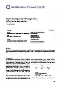
plane strain drawbead model the mesh is fixed in flow direction; perpendicular to the flow direction the mesh is free to move. The main advantages of this A.L.E.-formulation are that the grid refinements remain at their place and that the effects of sheet thinning can be described as well. For the grid is fixed in flow direction, there is no need to model a large mesh in contrast to the Lagrangian formulation where the sheet can be pulled out of the drawbead. In [9] it is proven that this 2D-model is a reliable tool to predict the effects of a drawbead. For one specific drawbead geometry the calculated D.B.R.F. and plastic thickness strain are printed as a function of the material displacement in figure 6.

50

Figure 6. Numerical results of the 2D analysis The plastic thickness strain and the D.B.R.F. reach their stationary value when a particle has been pulled through the entire drawbead [10]. For this specific drawbead geometry the steady state is reached after about 37 [mm] material displacement. The steady state value for the D.B.R.F. amounts 83 [N/mm] and for the plastic thickness strain -0.086. The steady state value of the lift force is 72 [N/mm].

4.2.

Equivalent drawbead model

In the equivalent drawbead model the geometry of the drawbead is replaced by a line on the tool surface, see figure 7. When an element passes this ‘drawbead line’ an additional D.B.R.F. and a plastic thickness strain are added to that element. At the same time the lift force is subtracted from the total blankholder force.

Figure 7. Principle of the equivalent drawbead

In the drawbead only the material flow in normal direction ‘n’ is responsible for all the appearing drawbead strain and force. The tangential component ‘t’ of the material flow does not give any contribution to the drawbead strain and force. Therefore the material flow will be split in a normal and a tangential component. For the equivalent drawbead model only the normal component will be taken into account. The equivalent drawbead co-ordinate system is defined with the xdb-axis normal to the drawbead and the ydb-axis parallel to the drawbead. The ydb-axis is also the plane strain direction of the 2D-drawbead analysis. Firstly the implementation of the lift force is looked at. The direction of this lift force is opposite to the direction of the blankholder force. When the blankholder is lifted by the drawbead lift force, the whole blankholder is lifted. From this it can be concluded that the appearing drawbead lift force is not a phenomenon on a local level but it influences the total deep drawing process. Therefore the lift force is subtracted from the total blankholder force in action. Secondly the implementation of the D.B.R.F. is focused on. The D.B.R.F. is history dependent, its value is a function of the material which already passed the drawbead. The force fdbrf to be added is a curve fit from this drawbead restraining force which is gained from a 2D-drawbead analysis or from experimental data. The fitted force increases exponentially until the steady state value is reached. When an element passes the equivalent drawbead the D.B.R.F. must be added to that element. This additional force is taken into account in the right hand side of the finite element equations as an extra body force, as can be seen in equation (11):

K ⋅ ∆u = ∆ f + f

dbrf

(11)

In this equation K is the stiffness matrix, ∆u is the incremental displacement vector, ∆f is the incremental force vector and fdbrf is the drawbead restraining force vector. Finally the implementation of the plastic thickness strain is described. When an element passes the equivalent drawbead a proportional plastic thickness strain is also added to that element. This plastic thickness strain is history dependent too. The strain to be added is also a curve fit from the drawbead thickness strain, which is gained from a 2D-drawbead analysis or from experimental data. To implement this additional strain in the equivalent drawbead model an extra stiffness term is added to the finite element equations:

(K − K ) ⋅ ∆u = ∆ f db

(12)

The additional stiffness term can be expressed in stresses:

K ⋅ ∆ u = ∆ f + ∫ B T ⋅ ∆σ db dV

(13)

V

The drawbead stress σdb must be estimated to solve equation (13). This estimation of the stresses can be calculated out of the prescribed plastic thickness strain and the boundary conditions [11], [12].

Two sets of simulations are performed to test the equivalent drawbead model. In the first set the equivalent drawbead algorithm is tested by pulling a strip material through a flat die and blankholder. An equivalent drawbead is placed on the tool surface. The outline of this test is depicted in figure 8. The applied D.B.R.F. and the plastic thickness strains are curve fits of the data depicted in figure 6. Three simulations are performed, in one simulation only the D.B.R.F. is prescribed, in one only the plastic thickness strain is prescribed and in the last simulation both the drawbead force and strain are prescribed. The results of these simulations are also depicted in figure 8. From the appearing strain in the material due to the prescribed D.B.R.F. it can be concluded that indeed the material is restrained by the equivalent drawbead. Also the changes in strain distribution due to a prescribed plastic thickness strain are well incorporated. From these results it can be concluded that the equivalent drawbead model works satisfactory for this test. 0

50

100

thickness strain

0.00 force -0.08

-0.16

strain force & strain original co-ordinate [mm]

Figure 8. Results of the simple strip test In the second set the deep drawing of a rectangular cup is simulated. An equivalent drawbead is placed at the long side of the cup. The applied D.B.R.F. and the plastic thickness strains are curve fits of the data depicted in figure 6. Four simulations are done. In the first simulation no drawbead is used. In the second simulation only a D.B.R.F. is applied. In the third simulation both the D.B.R.F. and the plastic thickness strain are prescribed. In the fourth simulation also the lift force is taken into account. The deformed mesh of the rectangular cup after 80 [mm] deep drawing is shown in figure 9a. The flange shapes of the four simulations are shown in figure 9b. The initial blank shape is also depicted in this figure. Applying a prescribed D.B.R.F. in the equivalent drawbead model results in a decrease in the draw-in at the long side, as was expected. When also the plastic thickness is prescribed the draw-in hardly differs from the simulation with only a prescribed D.B.R.F.. Also the strain changes are small. However it can be concluded that the effect of prescribing the plastic thickness strain is small which is caused by the very slow convergence behaviour. In the fourth simulation also a lift force is applied. The blankholder force becomes lower as a result of this lift force, and hence the material is less restrained to flow into the die. However the effect of adding a lift force is very small.

coordinates y-axis [mm]

200

drawbead

100

initial blank no drawbead force force & strain also lift force

0 0

b.

a.

100 200 coordinates x-axis [mm]

300

Figure 9a. Deformed mesh after 80 [mm] deep drawing Figure 9b. Results of the rectangular cup simulations 5.

Conclusions

In sheet metal forming the friction coefficient is not a constant, it depends on the local contact conditions. To achieve an accurate description of the friction a new friction model has been developed which accounts for this dependency. Applying the Stribeck friction model in a deep drawing simulation gives different results compared to the commonly used Coulomb friction model. The material behaviour is commonly described with the Hill yield criterion. Unfortunately this criterion is not always sufficient to accurately describe the material behaviour. To achieve a better material description a new yield function has been developed. This Vegter yield function directly uses the experimental results at multi-axial stress states. An equivalent drawbead model is developed which replaces the real drawbead geometry by a line on the tool surface to avoid an enormous increase in CPU-time. The model works satisfactory when only a D.B.R.F is prescribed, the model does not give the desired result when also the plastic thickness strain is prescribed. This is caused by the very slow convergence behaviour.

Acknowledgements The authors thank Hoogovens Research & Development for performing the drawbead experiments and their support in this research.

References [1] Schey J.A., “Tribology in Metalworking, Friction, Lubrication and Wear”, ASM, Metals Park, Ohio, USA, 1983 [2] Schipper D.J., “Transition in the lubrication of concentrated contacts”, Ph.D. thesis, University of Twente, Enschede, 1988 [3] Haar R. ter, “Friction in Sheet Metal Forming, the influence of (local) contact conditions and deformation”, Ph.D. thesis, University of Twente, Enschede, 1996

[4] Carleer B.D., J. Huétink, “Closing the Gap between the Workshop and Numerical Simulations in Sheet Metal Forming” Computational methods in applied sciences (proceedings eccomas ’96), J.-A. Désidéri, C. Hirsch, P. Le Tallec, E. Oñate, M. Pandolfi, J. Périaux and E. Stein, 1996, p. 554-560 [5] Vegter H., P. Drent, J. Huétink, “A planar isotropic yield criterion based on mechanical testing at multi-axial stress states”, Numiform ’95, S.F. Shen & P.R. Dawson, 1995, p. 345-350 [6] Carleer B.D., “Finite element analysis of the deep drawing process”, Ph.D. thesis, University of Twente, Enchede, 1997 [7] Pijlman H.H., “Implementation of the Vegter yield criterion in the Finite Element Program DIEKA”, master thesis, University of Twente, Enchede, 1996 [8] Wouters P., G. Montfort, J. Defourny, “Numerical simulations and experimental evaluation of the modifications of material properties in a drawbead”, Recent developments in Sheet Metal Forming Technology, M.J.M. Barata Marques, Lisbon, 1994, p. 389-401 [9] Carleer B.D., P.T. Vreede, M.F.M. Louwes, J. Huétink, ”Modelling Drawbeads with Finite Elements and Verification”, J. Mat. Proc. Tech., Vol. 45/1-4, 1994, p. 63-68 [10] Cao J., M.C.Boyce, “Drawbead penetration as a control element of material flow”, SAE 930517, Sheet Metal and Stamping Symposium, Detroit, 1993 [11] Meinders T., “Drawbead modelling in 3D deep drawing processes”, master thesis, University of Twente, Enschede, 1996 [12] Carleer B.D., T. Meinders, J. Huétink, “Equivalent drawbead model in finite element simulations”, conference proceedings Numisheet ’96, Detroit, 1996, p. 25-31