A major chal- lenge for these systems today is the limited radio frequency ... communication systems, the spatial structure is poorly de- ..... 8] Simon S. Haykin.
Recursive Algorithms for Estimating Multiple Co-Channel Digital Signals Received at an Antenna Array Shilpa Talwar
Arogyaswami Paulraj
Scienti c Computing Bldg. 460, Stanford University Stanford, CA 94305
Information Systems Lab. 133 Durand, Stanford University Stanford, CA 94305
Abstract We have recently proposed a new maximum likelihood approach for separating multiple co-channel digital signals received at an antenna array. This approach exploits the nite alphabet property of digital signals to simultaneously estimate the array response matrix A and symbol matrix S, given the data matrix X = AS. In [1, 2], we presented two e�cient block algorithms for computing the estimates: Iterative Least-Squares with Projection (ILSP) and Iterative Least-Squares with Enumeration (ILSE). These algorithms are based on the alternating projections technique whereby the ML criterion is minimized successively, rst with respect to the variable A, and then with respect to S. In this paper, we consider the recursive extensions of these algorithms. We also present a new approach which minimizes the ML criterion directly, assuming that the previous symbols have been estimated correctly. Simulation demonstrate the promising performance of these recursive techniques.
or special array geometry. Common high-resolution techniques for DOA estimation include MUSIC and ESPRIT [3, 4]. An optimum beamformer is then constructed from the corresponding array responses to extract the desired signals from interference and noise [5]. Although this twostep approach is quite successful, its performance depends strongly on the reliability of prior spatial information. In many situations of practical interest, this information is known imprecisely or unknown. For example, in wireless communication systems, the spatial structure is poorly de ned due to a highly variable propagation environment. However, prior knowledge of the temporal structure of the signals is available for these systems, and can be exploited for signal separation.
We have recently proposed a blind temporal approach that exploits the nite alphabet property of digital signals to simultaneously estimate the array response and symbol sequence of each signal. This approach is termed blind since it does not require prior knowledge of array responses or training signals for signal demodulation. The idea is to revisit data received at the array iteratively until a best t 1 Introduction of the array response and signal model is obtained. Two Wireless communication systems are witnessing rapid computationally e�cient block iterative algorithms, ILSP advances in volume and range of services. A major chal- and ILSE, are used to converge rapidly to array response lenge for these systems today is the limited radio frequency and signal estimates. spectrum available. Approaches that increase spectrum ef ciency are therefore of great interest. One promising apIn this paper, we consider the recursive extensions of proach is to use antenna arrays at the cell sites. Array pro- the block algorithms: Recursive Least-Squares with Processing techniques can then be used to receive and transmit jection (RLSP) and Recursive Least-Squares with Enumermultiple signals that are separated in space. Hence, multi- ation (RLSE). The recursive algorithms are used to estiple co-channel users can be supported per cell to increase mate the signals and track the array response matrix in a capacity. In this paper, we consider the separation problem time-varying environment. These algorithms require a good for digital signals received at an antenna array. The ar- initial estimate of A, which can be obtained from the block ray output consists of a superposition of signal waveforms algorithms or from a short set of training signals. We also plus additive noise. Our goal is to reliably demodulate each present a new recursive technique, Recursive Projection Upsignal in the presence of other co-channel signals and noise. date (RPU), that minimizes the ML criterion directly. This The traditional approach to this problem exploits the technique assumes that the previous symbols have been despatial structure of the antenna array. The signals are es- modulated correctly or with a low error rate. Simulation timated by a two-step procedure. First, the directions of results show that the proposed direct approach is more roarrival (DOAs) of the signals are determined using prior bust that alternating projections approach used in RLSP knowledge of the array response structure : calibration data and RLSE.
2 Problem Formulation
f�j; �j3; : : :; �j(L ? 1)g for complex signals. These corre-
spond to the important cases of PAM and QAM modulation Consider d narrowband signals impinging at an array of formats. Now, assuming that the signals are symbol-synchronous, m sensors with arbitrary characteristics. It is well known that the m � 1 vector of sensor outputs, x� (t), in the absence we perform matched ltering on (3) over each symbol period T, to obtain the following equivalent discrete representation of multipath, is given by of the data d X d X x�(t) = pka(�k )sk (t) + v� (t) (1) x (n) = pk ak bk (n) + v(n): (6) k=1 where pk is the amplitude of the kth signal, a(�k ) is the array response vector to a signal from direction �k , sk (�) is the kth signal waveform, and v� (�) is white complex symmetric Gaussian noise. However, in a wireless scenario, there are usually multiple re ected and di�racted paths from the source to the array. These paths arrive from di�erent angles, and with di�erent attenuations and time delays. Hence, the array output becomes
k=1
The noise term, v(n), is a discrete white complex symmetric Gaussian process. Using the techniques of [6], it is easily shown that the output of the matched lter is a su�cient statistic for determining the transmitted symbols. We can rewrite (6) in matrix form x(n) = As(n) + v(n) (7) where x(n) is the ltered data, s(n) = [b1(n) : : : bd (n)]T , q d k XX (n) is additive white noise, and A is an m � d matrix of a(�kl ) pk �kl sk (t ? �kl ) + v�(t) (2) varray x� (t) = responses scaled by the signal amplitudes k=1 l=1 A = [p1 a1 : : : pd ad ]: where qk is number of subpaths for the kth signal, and �kl and �kl are, respectively, the attenuation and time delay The problem addressed in this paper is the estimation of corresponding to lth subpath. We assume that the propa- the symbol vector s(n), given the ltered array output x(n), gation delays associated with these paths is much smaller and a good estimate of A. than the inverse bandwidth of the signals. The delays can thus be modeled as phase-shifts under the narrowband assumption. The new data model can be written as 3 Block Algorithms d X
Assuming that the channel is constant over N symbol periods, we can obtain a block formulation of the data k=1 X(N) = AS(N) + V(N) (8) where ak is now the total array response vector where X(N) = [x(1) : : : x(N)], S(N) = [s(1) : : : s(N)], Dk X ? j! c �kl ak = �kle a(�kl ); (4) and V(N) = [v(1) : : : v(N)]. The objective in block estimation is to jointly estimate A and S(N), given only X(N). l=1 Since the array response matrix is assumed to be completely and !c is the carrier frequency. The only di�erence between unknown, the block approach is termed blind. Equations (1) and (3) is that the spatial structure of the From Equation (7), we see that the digital signals can array response vector ak cannot be exploited if the number be modeled as unknown deterministic sequences corrupted of paths is larger than the number of sensors. However, the by white Gaussian noise. The log likelihood function of the signal structure can still be exploited, ltered data is given as N N X X (5) sk (t) = bk (n)g(t ? nT) L = ?const ? mN ln(2�2 ) ? 2�1 2 kx(n) ? As(n)k2 : n=1 n=1
x� (t) =
pk ak sk (t) + v� (t)
(3)
where N is the number of symbols in a data batch (burst), fbk (�)g is the symbol sequence of the kth user, T is the symbol period, and g(�) is the unit-energy signal waveform of duration T. For simplicity, we assume that the symbols belong to the alphabet = f�1; �3; : : :; �(L ? 1)g for real signals, and = f�1; �3; : : :; �(L ? 1)g �
In maximumlikelihood estimation, we maximizes L with respect to the unknown parameters A and s(n); n = 1 : : :N;. This yields the following separable least-squares minimization problem min kX(N) ? AS(N)k2F (9) A;S(N )2
in variables A and S(N) which are respectively continuous and discrete. It is proved in [7] that the minimization can be carried out in two steps. First, we minimize (9) with respect to A since it is unconstrained A^ = X(N)S(N)y = X(N)S(N)� (S(N)S(N)�)?1 : (10) Then, substituting A^ back into (9), we obtain a new criterion which is a function of S(N) only ? � k2 ; min k X (N) P (11) S(N ) F S(N )2
where P?S (N )� = IN ? S(N)� (S(N)S(N)� )?1S(N). The global minimum of (11) can be obtained by enumerating over all possible choices of S(N). But, this search has an exponential complexity in the number of symbols N (and the number of signals d), and can be computationally prohibitive, even for modest size problems. Thus, it is desirable to consider sub-optimal algorithms that have a lower computational complexity. The algorithms, ILSP and ILSE, are e�cient iterative algorithms that minimize (9) by taking advantage of the estimator being separable in its unknowns. Given an initial estimate of A, we iterate using an alternating minimization technique: minimize the ML criterion with respect to S(N) and then with respect to A, at each step. We continue this iterative process until we converge to a local or global minimum. We see that minimization with respect to A, holding S(N) xed, is a standard least-squares problem. The rst algorithm, ILSP, minimizes with respect to S(N) using least-squares, and then projecting each element of the solution to its closest discrete value. It performs very well with little or no a priori spatial information, and can be used to initialize the second algorithm. Dropping the index N, the algorithm is summarized as follows.
Iterative Least-Squares with Projection (ILSP) 1. Given A0 , k = 0
2. k = k + 1 � Sk = (A�k?1Ak?1)?1 A�k?1X � Project [Sk ]ij to closest discrete values � Ak = XS�k (Sk S�k )?1 3. Continue until (Ak ? Ak?1) = 0 The second algorithm, ILSE, exploits the data model more fully at the expense of higher computational complexity. Minimization with respect to S is done by enumerating over each column independently since 2 min min kx(1) ? As(1)k2 + : : : S2 kX(N) ? AS(N)kF = s(1) 2
For a su�ciently good initialization, this algorithm converges rapidly to the ML estimate of the array responses and signal symbol sequences.
Iterative Least-Squares with Enumeration (ILSE) 1. Given A0 , k = 0 2. k = k + 1 � Minimize (12) for Sk (Enumeration) � Ak = XS�k (Sk S�k )?1 3. Continue until (Ak ? Ak?1) = 0
4 Recursive Algorithms In this section, we consider two classes of recursive algorithms for estimating the received signals. In recursive estimation, we are interested in solving the following minimization problem at symbol period n 2
min k(X(n) ? AS(n))B(n) 12 kF
A;s(n)2
(13)
where X(n) = [X(n ? 1) x(n)], S(n) = [S(n ? 1) s(n)], and B(n) = diag(�n?1; �n?2; : : :; 1) is a diagonal weighting matrix for some 0 < � < 1. Our objective is to compute s(n) and A(n), assuming that a good estimate of S(n ? 1) (or equivalently A(n ? 1)) is available. For convenience, we consider the real alphabet = f�1; �3; : : :; �(L ? 1)g. It is easily shown that the detection of d complex signals is equivalent to 2d real signals. The exponential weighting is used to de-emphasize old data in a time-varying environment. The \fading memory" least-squares solution for A(n) is given by
A(n) = X(n)B(n)S�(n)(S(n)B(n)S� (n))?1
(14)
which can be updated recursively (see [8]), � A(n) = A(n ? 1) + �(x+(n)s�?(n)AP(n(n??1)1)ss(n)) (n) � s (n)P(n ? 1): (15) In the above Equation, P(n), de ned as P(n) = (S(n)B(n)S� (n))?1 , can also be expressed recursively as � s(n)s�(n)P(n ? 1) � ; P(n) = �1 P(n ? 1) ? P(n� +? s1)�(n) P(n ? 1)s(n) P(0) = I:
In addition, we de ne H(n) = X(n)B(n)S� (n), so that we can rewrite A(n) = H(n)P(n) in Equation (14). Using this we are now ready to consider the two classes of 2 + s(min kx(N) ? As(N)k (12) framework, recursive algorithms. N )2
4.1 Class A
We can equivalently maximize
2
1 2P (19) max k X (n) B (n) The rst class of recursive algorithms includes the natB(n) 21 S(n)� kF s(n)2
ural extensions of the two block algorithms presented in Section 3. The algorithms in this class alternate between which can be expressed in terms of the trace operator estimating s(n), and then updating A(n), at each symbol max tr[B(n) 21 PB(n) 21 S(n)� B(n) 21 X(n)� X(n)]: (20) period. For each data vector x(n), we rst estimate s(n) s(n)2
by minimizing Using X(n) = [X(n ? 1) x(n)], we can partition 2 � � � ^s(n) = s(min k x (n) ? A (n ? 1) s (n) k (16) � F n)2
X� (n)X(n) = X x(�n(n?)X1)(Xn(?n ?1) 1) X x(�n(n?)x1)(nx)(n) : (21) using either the least-squares with projection approach (RLSP) or the enumeration approach (RLSE). This step re- From Equation (18), we can write quires O(md2 ) ops for least-squares or O(mdLd ) ops for B(n) 21 PB(n) 21 S(n)� B(n) 21 = B(n)S(n)� P(n)S(n)B(n); enumeration. Then, A(n) is computed using Equation (15), (22) which requires O(md) ops. The enumeration approach is more robust for low SNR's, and is thus recommended when- and by noting that the weighting matrix can be expressed � � ever computationally feasible (for small values of d). The as (23) B(n) = �B(n0 ? 1) 01 ; following recursive algorithmhas complexity O(mdLd ) ops per snapshot: and S(n) = [S(n?1) s(n)], we can partition (22) in a similar Recursive Least Squares with Enumeration (RLSE) fashion as (21). Multiplying Equations (21) and (22), and using proper1. Given A(n ? 1) ties of the trace, we can rewrite the argument of the trace operator in (20) as 2. n = n + 1 �2H(n ? 1)P(n)H� (n ? 1) + �H(n ? 1)P(n)s(n)x� (n) � Minimize (16) for ^s(n) (Enumeration) +�P(n)H� (n ? 1)x(n)s� (n) + P(n)s(n)x� (n)x(n)s� (n): � Update A(n) using (15) (RLS) (24) It is easily seen that H(n) can be updated recursively 3. Continue with the next snapshot H(n) = �H(n ? 1) + x(n)s(n)� ; (25) 4.2 Class B and thus, (20) reduces to In this class of algorithms, we minimize Equation (13) max tr[H(n)P(n)H� (n)]: s(n)2
jointly over A(n) and s(n). This is achieved by substituting the weighted least-squares solution for A(n), given by Since A(n) = H(n)P(n), we estimate s(n) by maximizing Equation (14), back into the original minimization criterion to yield a new criterion ^s(n) = smax tr[A(n)H� (n)]: (26) (n)2
2 F
min kX(n)B(n) 21 P?B(n) 21 S(n)� k ;
Substituting H� (n) = S(n)B(n)X� (n) in (26), it follows that we choose1 s(n) to maximize the correlation between 1 2 and X(n)B(n) 2 . A (n) S (n) B (n) ? where PB(n) 21 S(n)� = In ? PB(n) 12 S(n)� , and PB(n) 12 S(n)� is In Equation (26), we compute A(n) and H(n) for each of a d-dimensional projection matrix de ned by the rows of the Ld possible vectors s(n) 2 . This is done recursively 1 S(n)B(n) 2 using Equations (15) and (25), and hence the computation requires O(mdLd ) ops. Next, we compute the diagonal 1 1 PB(n) 12 S(n)� = B(n) 2 S(n)�(S(n)B(n)S(n)� )?1 S(n)B(n) 2 : entries of A(n)H� (n) since we are only interested in the (18) trace of the product. Computing the trace for all possible Note that the main di�erence between the criterion in Equa- vectors s(n) also requires O(mdLd ) ops. Hence, this retion (17) and the block ML criterion in Equation (11) is that cursive approach has computational complexity O(mdLd ), the minimization in (17) is over s(n) only, since S(n ? 1) which is the same as RLSE for large d. However, we obtain is assumed to be known. Hence, recursive minimization of better signal estimates using this approach. The algorithm can be summarized as follows. the ML criterion is computationally more tractable. s(n)2
(17)
Recursive Projection Update (RPU) 1. Given A(n ? 1) and H(n ? 1)
0.055 0.05
2. n = n + 1 � Maximize (26) for ^s(n) � Update A(n) and H(n) 3. Continue with the next snapshot
0.045 0.04
SER
0.035 0.03 0.025
5 Simulation Results
0.02
In this section, we study the performance of the algorithms presented in this paper via two sets of simulatons. In the rst set, we consider the block algorithms for a block size of N = 100. We assume an array of m = 4 sensors, with 2 digitally modulated BPSK signals of equal powers, arriving from [0; 5]� relative to array broadside. Starting with A0 = Im�d , we rst estimate A^ and S^ using ILSP. The estimate A^ is then used to initialize ILSE for improved array response and signal estimates. This blind estimation process is repeated 104 times, each time over a di�erent noise realization. Hence, a total of 106 bits are estimated for each signal. We see from Equation (12) that in ILSE, we make a joint decision on all d bits in each snapshot s(n); n = 1 : : :N. Hence, it is convenient to consider the Snapshot Error Rate (SER), which is the probability that s(n) does not equal ^s(n). 0
10
−1
10
0.015 1.14e−2 0.01 0.005 0
50
100 150 Symbol Period (n)
200
250
Figure 2: Snapshot Error Rate Pro le for RPU SER attainable by any algorithm. The `�' and `�' indicate the SER performance of the blind algorithms, initialized with A0 = Im�d . The plot shows that there is virtually no di�erence in the performance of the blind algorithms as compared to the non-blind approach. In the next set of simulations, we study the performance of recursive algorithms. We use d training signals, de ned by the columns of the full-rank matrix Sd , 2 +1 +1 +1 : : : +1 3 66 +1 ?1 +1 : : : +1 77 Sd = 66 +1. +1. ?.1 : :. : +1. 77 ; 4 . . . . . 5 .
.
.
+1
+1
+1
.
.
: : : ?1
to obtain an initial estimate A0 . For simplicity, we choose � = 1. As in the previous set, we rst consider the simple scenario with 2 BPSK signals arriving from 0 and 5 degrees. At 3 dB SNR, we estimate N = 250 snapshots using RLSE and RPU. We average the results over 104 such runs, so that a total of 2:5 � 106 bits per signal are estimated. The BERs achieved by both the algorithms are equal: 1:45 � 10?2 for each signal, although the number of bits in error is slightly larger for RLSE. The SER for the two algorithms is also 1:45�10?2. In Figure 2, we plot the SER using RPU at each symbol period n; n = 1 : : :N. The SER plot using RLSE is virtually identical for this scenario. We observe that the Figure 1: Snapshot Error Rate for ILSP and ILSE SER is high initially since the estimate of A is poor. But as In Figure 1, we compare the performance of blind algo- n increases, this estimate improves and the SER decreases. rithms to the case where the array response matrix is com- After n = 120, the SER converges to about 1:14 � 10?2, pletely known. The dashed and the solid lines indicate the the theoretical SER for known A, as shown in Figure 1. theoretical SER for ILSP and ILSE respectively, assuming Finally, we make the current scenario more di�cult scenario that A is known (see [9]). For the ML minimization cri- by adding another signal at 10 degrees with 3 dB SNR. Also, terion (9), the SER curve for ILSE represents the lowest we reduce N = 100 to ease the computational burden. The ILSP
−2
ILSE
SER
10
−3
10
−4
10
−5
10
0
1
2
3
4 SNR (dB)
5
6
7
8
BERs achieved by RLSE and RPU are given in Table 1. [6] H.L. Van Trees. Detection, Estimation and Modulation We see that RPU yields lower BERs than RLSE. Theory, volume I. Wiley, New York, 1968. [7] G. Golub and V. Pereyra. The Di�erentiation of Pseudo-Inverses and Nonlinear Least Squares ProbBit Error Rate lems Whose Variables Separate. SIAM J. Num. Anal., Alg. s1 s2 s3 10:413{432, 1973. RLSE 2:88 � 10?2 5:26 � 10?2 2:59 � 10?2 RPU 2:66 � 10?2 4:92 � 10?2 2:39 � 10?2 [8] Simon S. Haykin. Introduction to Adaptive Filters. Macmillan, New York, 1984. Table 1: Bit Error Rate for RLSE and RPU [9] S. Talwar and A. Paulraj. Performance Analysis of Blind Digital Signal Copy Algorithms. In Proc. MILCOM, volume I, pages 123{128, 1994.
6 Conclusions
We have presented a new approach for estimating of synchronous co-channel digital signals received at an antenna array. This approach exploits the nite alphabet property of digital signals to compute signal estimates in a timevarying propagation environment. The extension of these algorithms to the asynchronous case is straighforward. In ILSP (or RLSP) and ILSE (or RLSE) respectively, the projection and enumeration steps are replaced by a sequence estimation step, which can be solved via the Viterbi algorithm. An important direction for future work is extending this approach to multipath channels with large delay spread, which are more realistic in a wireless setting.
References [1] S. Talwar, M. Viberg, and A. Paulraj. Blind Estimation of Multiple Co-Channel Digital Signals Arriving at an Antenna Array. In Proc. 27th Asilomar Conference on Signals, Systems and Computers, volume I, pages 349{ 353, 1993. [2] S. Talwar, M. Viberg, and A. Paulraj. Blind Estimation of Multiple Co-Channel Digital Signals Using an Antenna Array. IEEE Signal Processing Letters, (1)2:29{31, Feb 1994. [3] R. O. Schmidt. A Signal Subspace Approach to Multiple Source Location and Spectral Estimation. PhD thesis, Stanford University, Stanford, CA, 1981. [4] A. Paulraj, R. Roy, and T. Kailath. Estimation of Signal Parameters via Rotational Invariance Techniques - ESPRIT. In Proc. Nineteenth Asilomar Conf. on Circuits, Systems and Comp., 1985. [5] B. Ottersten, R. Roy, and T. Kailath. Signal Waveform Estimation in Sensor Array Processing. In Proc. Twenty-Third Asilomar Conf. on Signals, Systems and Computers, pages 787{791, 1989.