Reducing Uncertainty of Low-Sampling-Rate Trajectories - CiteSeerX

Reducing Uncertainty of Low-Sampling-Rate Trajectories Kai Zheng 1 , Yu Zheng 2 , Xing Xie 2 , Xiaofang Zhou 1,3 1

School of Information Technology and Electrical Engineering, The University of Queensland, Brisbane 4072, Australia, {kevinz,zxf}@itee.uq.edu.au 2 Microsoft Research Asia, Beijing, China, {yuzheng, xingx}@microsoft.com 3 School of Information, Renmin University of China, China Key Lab of Data Engineering and Knowledge Engineering, Ministry of Education,China

Abstract—The increasing availability of GPS-embedded mobile devices has given rise to a new spectrum of location-based services, which have accumulated a huge collection of location trajectories. In practice, a large portion of these trajectories are of low-sampling-rate. For instance, the time interval between consecutive GPS points of some trajectories can be several minutes or even hours. With such a low sampling rate, most details of their movement are lost, which makes them difficult to process effectively. In this work, we investigate how to reduce the uncertainty in such kind of trajectories. Specifically, given a low-sampling-rate trajectory, we aim to infer its possible routes. The methodology adopted in our work is to take full advantage of the rich information extracted from the historical trajectories. We propose a systematic solution, History based Route Inference System (HRIS), which covers a series of novel algorithms that can derive the travel pattern from historical data and incorporate it into the route inference process. To validate the effectiveness of the system, we apply our solution to the map-matching problem which is an important application scenario of this work, and conduct extensive experiments on a real taxi trajectory dataset. The experiment results demonstrate that HRIS can achieve higher accuracy than the existing map-matching algorithms for low-sampling-rate trajectories.

I. I NTRODUCTION The proliferation of GPS-enabled devices has given rise to a boost of location-based services, by which users can acquire their present locations, search interesting places around them and find the driving route to a destination. Meanwhile, location-based online services such as Google Latitude and Foursquare allow users to upload and share their locations are getting popular. These services and products have accumulated huge amount of location trajectory data, which inspires many applications such as route planner [1], hot route finder [2], traffic flow analysis [3], etc, to leverage this rich information to achieve better quality of services. A location trajectory is a record of the path of a variety of moving objects, such as people, vehicles, animals and nature phenomena. But in practice, a large portion of these trajectory data is of low-sampling-rate, i.e., the time interval between consecutive location records is large. For instance, most taxis in big cities are equipped with GPS sensors which enable them to report time-stamped locations to a data center periodically. However, to save energy and communication cost, these taxis usually report their locations at low frequency. According to our statistical analysis on the GPS data collected from 10,000+

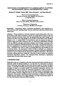
taxies in a large city, more than 60% of the taxi trajectories are of low-sampling-rate (the average sampling interval exceeds 2 minutes). Besides, low-sampling-rate trajectories can also be generated from web applications. In Flickr a set of geotagged photos can be regarded as a location trajectory because each photo has a location tag and a timestamp respectively corresponding to where and when the photo was taken. The average time intervals of this kind of trajectories can be tens of minutes or even hours. With such a low sampling rate, most detail information about the exact movement of objects is lost and great uncertainty arises in their routes. Consider the trajectories of vehicles in Figure 1 as an example. If the sampling rate of the trajectory Ta is high, we can tell the route it travelled unambiguously. However, when the sampling rate is low (i.e., only solid points can be seen), how Ta travels between the consecutive GPS observations is not certain any more. In some other kinds of trajectories, such as the one from geotag photos or migratory birds, where the location records are very sparse, uncertainty becomes even more significant. This kind of uncertainty will severely affect the effectiveness and efficiency of subsequent process such as indexing [4][5][6], querying and mining [7]. Motivated by this, in this paper we aim at reducing uncertainty for low-sampling-rate trajectories. Specifically, given a low-sampling-rate trajectory, our goal is to infer its possible routes. The results of our work can be beneficial for a lot of practical applications, such as traffic management [3], trip mining from geo-tap photos [8], scientific study of animal behaviors or hurricane movement [9], etc. The methodology adopted in this work is to take full advantage of the information in the historical trajectory data. Real spatial databases usually archive a huge amount of historical trajectories, which can exhibit patterns on how moving objects usually travel between certain locations. Therefore, given a low-samplingrate trajectory as the query, it is possible to discover some routes which are more popular than others. Then we suggest these popular routes as our estimation of its real path. In this way, the enormous possible routes of the query are cut down to a few popular routes, and consequently the uncertainty is reduced.

• Ta Tb Tc

a

b c

Fig. 1: Uncertainty in low-sampling-rate trajectories

A. Motivational Observations Why is it feasible to reduce the uncertainty of low-samplingrate trajectories by leveraging historical data? At the heart of the motivation for this work, there are two important observations based on our analysis on real datasets. Observation 1: Travel patterns between certain locations are often highly skewed. Though the possible routes between two locations far away to each other are usually enormous, only a few of them are travelled frequently. This is due to the fact that, when people travel, they often plan the route based on the experience of their own or others, rather than choosing a path randomly. The skewness of travel pattern distribution makes it feasible to distinguish the possible routes based on their popularity. Observation 2: Similar trajectories can often complement each other to make themselves more complete. Trajectories are samples of objects’ movement, which are inherently incomplete. Given a set of low-sampling-rate trajectories that travel along the similar routes, there is no way to tell their exact path if we look at them in an isolated manner, since each of them is incomplete. Yet an interesting observation is that, if we consider these trajectories collectively, they may reinforce each other to form a more complete route. Consider Figure 1 as an example, in which there are another two lowsampling-rate trajectories Tb , Tc that travel on the same route as Ta . As we can see, their sample locations interleave with each other, which makes it possible to know their complete route if we can find a way to aggregate them together.

For a more practical solution, we propose to process a given query in three steps. Firstly, we divide the whole query into a sequence of sub-queries and search for the reference trajectories that can give hints on how each subquery travels. Then we infer the local routes for each subquery by considering the reference trajectories in a collective manner. At last, we connect consecutive local routes to form the global routes and return the ones with the highest scores to the users. As a summary, the essence of the route inference approach in this paper is to extract the travel pattern from history, and infer the possible paths of the query by suggesting a few popular routes. Compared to the original number of possible routes, the uncertainty existing in the query trajectory is reduced significantly in this way. To summarize, the major contributions of this paper lie in the following aspects: •

•

•

•

•

B. Challenges and Contributions Intuitively, given a low-sampling-rate query trajectory, one can simply search for the historical trajectories that pass by all the points of the query. Then we find the routes that have been travelled by the most historical trajectories. However, this method cannot work well in practice for two reasons. • Data sparseness. Since the query can have arbitrary locations, we usually cannot find any historical trajectory that matches the whole part of the query very well. Even if we can, the amount may not be enough to support the inference. Hence if we simply group the trajectories by their routes, none of them can fall in the same group in most cases, which results in a set of non-distinguishable possible routes.

Data quality. In a real moving object database, the quality of historical data cannot be guaranteed, i.e., highsampling-rate and low-sampling-rate trajectories co-exist. As a consequence, the exact routes of many historical trajectories are also unknown. So how to deal with the historical data with varies quality is a difficult problem we need to address.

•

We present a new methodology of inferring the possible route for a low-sampling-rate trajectory by leveraging the information from historical trajectories. We develop a systematic solution, history based route inference system (HRIS), which covers the whole process of transforming a given query to a set of possible routes. We introduce the concept of reference trajectories, which are obtained from the historical data, either natively existing or artificially constructed, and could give hints on how moving objects usually travel between certain locations. We propose two local route inference algorithms, traverse graph based approach and nearest neighbor based approach, which considers all the reference trajectories in a collective way. A hybrid approach that combines the merits of the two algorithms is also proposed so as to achieve better performance when the distribution of historical data fluctuates significantly. We define a reasonable scoring function for the global routes which incorporates the popularity of each local route as well as the confidence of the connections between them. We build our system based on a real-world trajectory dataset generated by 33,000+ taxis in a period of 3 months, and evaluate the effectiveness of our system by using map-matching as a case study. The results show that the routes suggested by our system is more similar with the ground truth than the existing map-matching algorithms for low-sampling-rate trajectories.

The remainder of this paper is organized as follows. In Section II we introduce the necessary background and give an overview of our whole system. Then we detail the route inference component in Section III, followed by our exper-

TABLE I: A list of notations Notation R r T T Tq , qi Ci Pi Ri f (Ri ) g(Ri , Rj ) s(R)

Definition A route on the road network A road segment A trajectory A set of trajectories The query trajectory and its i-th point The set of reference trajectories between qi and qi+1 The set of reference points between qi and qi+1 The set of local routes between qi and qi+1 the popularity of local route Ri The transition confidence from local route Ri to Rj The score of global route R

Problem Statement: Given an archive of historical GPS trajectories A, an underlying road network G, a low-samplingrate query trajectory Tq , we aim to suggest K possible routes of Tq by leveraging the information learned from A. B. Architecture Figure 2 shows the architecture of our system, which is comprised of two components: preprocessing and route inference. The first component operates offline and only needs to be performed once unless the trajectory archive or road network is updated. The second component is the key part of our system, and should be conducted on-line based on the query specified by a user.

imental observations in Section IV. Finally we position our work with respect to the related literature in Section V and draw a conclusion in Section VI. A partial list of notations used in this paper are summarized in Table I.

Low-sampling-rate Query Trajectory

Reference Search Indexing

R-tree Index

II. S YSTEM OVERVIEW In this section, we first clarify some terms used in this paper, and then briefly introduce the architecture of our system.

Map Matching

Simple Reference Search

Spliced Reference Search

Reference Trajectories

Trajectory Archive Local Route Inference Candidate Edges

A. Preliminaries In this subsection, we will gather the preliminaries necessary for the development of our main results, and state our problem. Definition 1 (GPS Trajectory): A GPS trajectory T is a sequence of GPS points with the time interval between any consecutive GPS points not exceeding a certain threshold ∆T , i.e., T : p1 → p2 → · · · → pn , where 0 < pi+1 .t − pi .t < ∆T (1 ≤ i < n). ∆T is called the sampling interval. This paper focuses on low-sampling-rate trajectories, of which ∆T is large. But the concept of ’high/low sampling rate’ is very subjective and cannot be defined in a strict form. Based on our observations and experiments on real datasets, we consider a trajectory with ∆T > 2min as low-samplingrate trajectory, since most traditional map-matching algorithms become less effective on such kind of trajectories. Definition 2 (Road Segment): A road segment r is a directed edge that is associated with two terminal points (r.s, r.e), and a list of intermediate points describing the segment using a polyline. Each road segment has a length r.length and a speed constraint r.speed which is the maximum speed allowed on this road segment. Definition 3 (Road Network): A road network is a directed graph G(V, E), where V is a set of vertices representing the intersections and terminal points of the road segments, and E is a set of edges representing road segments. Definition 4 (Route): A route R is a set of connected road segments, i.e., R : r1 → r2 → ... → rn , where rk+1 .s = rk .e, (1 ≤ k < n). The start point and end point of a route can be represented as R.s = r1 .s and R.e = rn .e. Definition 5 (Candidate Edge): The candidate edges of point p is the set of road segments whose distance with p is below a certain threshold ε, where the distance between a point p and a road segment r is defined as dist(p, r) = minc∈r d(p, c).

Graph based Approach

Nearest Neighbor based Approach

Trip Partition Route Scoring GPS Logs Global Route Inference

Preprocessing

Route Inference

Fig. 2: System overview 1) Preprocessing Component: To improve the quality of trajectory archive and facilitate the subsequence process, we perform some preprocessing before it is utilized by the route inference component. Trip Partition. In practice, a GPS log may record an object’s movement for a long period, during which it could travel from multiple sources to multiple destinations. Therefore to better utilize these historical data, we segment the GPS trajectories into effective trips, which is a route having one specific source and destination. If the object is stationary over a relatively long time, it usually implies the end of one trip and also the start of the next trip. This phenomenon can be well captured by the concept of stay point [10], which is a geographical region where a moving object stays over a certain time interval. So for each historical trajectory in the archive, we detect its stay points and then remove the GPS point belonging to the stay points, after which the trajectory will be naturally split into several trips. Map Matching. Due to GPS measurement error, the observation of a GPS point does not reflect its true position accurately. In this step, we align the observed GPS points onto the road segments by applying existing map-matching techniques. Indexing. A real moving object database usually archives tens of thousands of trajectories and millions of GPS points,

which prohibits us to search them sequentially. To enhance the performance of our system, we utilize R-tree to organize all the GPS points. 2) Route Inference Component: This is the key component of our system, which will process a given query in three phases: Reference Trajectory Search. Apparently not all the historical trajectory are relevant to the query. In this phase, we use the concept of reference trajectory to describe those historical trajectories that are useful for inferring the possible routes of the query. Ideally, the reference trajectories should travel by similar path with the query. However, due to data sparseness, normally we cannot find enough trajectories that are similar with the whole query. For this reason, we propose to partition the query into a sequence of consecutive location pairs, and search for the reference trajectories in each local area. Local Route Inference. In this step, we perform the local route inference based on the reference trajectories for each consecutive location pair of the query. To this end, two independent approaches are proposed. The traverse graph based approach constructs a conceptual graph by using the road segments travelled by some reference trajectories, and perform the inference based on this graph. The nearest neighbor based approach algorithm adopts a heuristic way to transfer from one reference point to its nearest neighbors until the destination (i.e., qi+1 ) is reached. Besides, to achieve better effectiveness and efficiency, a hybrid approach combining the advantages of the two methods is also presented. Global Route Inference. In the last step, we infer the global possible routes for the whole query by connecting consecutive local routes. To distinguish the global routes, we propose a scoring function by incorporating the popularity of each local route as well as the confidence for connecting them. Finally, we devise a dynamic programming algorithm to get the top-K global routes in terms of their scores efficiently. III. ROUTE I NFERENCE In this section, we detail the three phases of route inference component. A. Reference Trajectory Search Though spatial databases archive a large amount of trajectories, it is neither effective nor efficient to use them all for a specific query. Intuitively, we only need to utilize the ones in the surrounding area of the query since the relationship between two trajectories faraway from each other is usually weak. In this paper, we use the notion of reference trajectory to model those historical trajectories that can be useful for the route inference. Simple reference trajectories natively exist in the archive while spliced reference trajectories are constructed from two historical trajectories. In the rest of this paper, we use reference and reference trajectory interchangeably. 1) Simple Reference Trajectory: Formally, the simple reference trajectory is defined as follows. Definition 6 (Simple Reference Trajectory): Let nn(q, T ) denote the nearest point of trajectory T with respect to point q, i.e., nn(q, Tk ) = arg minp∈T {d(p, q)}. Given

a radius φ > 0, trajectory Tk is a simple reference trajectory with respect to the pair hqi , qi+1 i, where qi , qi+1 ∈ Tq , if there exits a sub-trajectory Tik = (pm , pm+1 , ..., pn ) ⊆ Tk such that, 1) pm = nn(qi , Tk ) and pn = nn(qi+1 , Tk ). 2) d(pm , qi ) ≤ φ and d(pn , qi+1 ) ≤ φ. 3) ∀p ∈ Tik , d(p, qi ) + d(p, qi+1 ) ≤ (qi+1 .t − qi .t) · Vmax , where Vmax is the maximum allowed speed of the road network. In the above definition, the first and second conditions require the trajectory to be close enough to qi and qi+1 , while the third condition guarantees that the query object is able to travel from qi to qi+1 via the route of the reference. We use Figure 3a to illustrate the intuition of this concept. T1 and T2 are simple reference trajectories with respect to hqi , qi+1 i as they satisfy all the conditions of Definition 6. T3 is not a reference trajectory as it does not fall inside the circle centered at qi+1 (i.e., does not satisfy the condition 2). T4 is not a simple reference trajectory either, since there is a point a ∈ T4 that violates the condition 3. T1 T2

qi

qi 1 T3

T4

a

(a) Simple reference trajectory T4 1

qi

qi 1

2

e

T3

T2

T1

(b) Spliced reference trajectory

Fig. 3: Reference trajectory Given a pair hqi , qi+1 i, we can search for the simple reference trajectories efficiently with the help of R-tree index that is already built in the preprocessing component. First, we issue two range query with radius of φ at qi and qi+1 respectively to retrieve all the trajectories that pass by either qi or qi+1 . Then by joining the two sets of range query results, we get a list of candidate trajectories that pass by both qi and qi+1 . Finally, the simple reference trajectories can be obtained by checking these candidates against the condition 3. 2) Spliced Reference Trajectory: In some cases such as an area with sparse historical data, the requirement for a trajectory to qualify a simple reference is too strict, which makes the number of obtained reference trajectories too small to support our inference. To address this problem, in this part we extend the concept of reference to include another kind of trajectories. Consider Figure 3b where neither T1 nor T2 is a simple reference. But if we splice them together, a virtual trajectory T3 will be formed, which actually is a good reference for estimating the true path of the query. Based on

this observation, we propose the notion of spliced reference trajectory. Definition 7 (Spliced Reference Trajectory): Given two trajectories Ta , Tb which are not simple reference trajectories w.r.t. hqi , qi+1 i, trajectory T = (p1 , ..., pm , pm+1 , ..., pn ) is a spliced reference trajectory w.r.t. hqi , qi+1 i, if 1) T satisfies all the conditions of Definition 6. 2) (p1 , ..., pm ) ⊆ Ta , (pm+1 , ..., pn ) ⊆ Tb . 3) d(pm , pm+1 ) ≤ e, where e is a user-specified threshold, and hpm , pm+1 i is called the splicing pair of T . Apparently, T3 in Figure 3b is a spliced reference. Essentially, a spliced reference is the mixture of two trajectories T1 (coming from qi ) and T2 (heading towards qi+1 ) which have some overlap. Even though neither T1 nor T2 pass by both qi and qi+1 , joining them together can still give hints on how people usually travels between qi and qi+1 . On the first sight, one may ask why we do not simply use a very large search radius to include as many simple reference trajectories as possible. However, it may include too many irrelevant trajectories, the ones far away from both qi and qi+1 . This kind of trajectories is very unlikely to be useful, and even worse, they may interfere the inference process. As we can see from Figure 3b, T4 will be regarded as a reference if we expand the radius from φ1 to φ2 , but it is unreasonable to leverage T4 to estimate the route from qi to qi+1 as it is too far away from them. The search for spliced reference trajectories can be performed as follows. First, the same as the reference search, we obtain two sets of candidate trajectories by issuing two range queries and removing the simple reference trajectories. Then we find all the splicing pairs by performing on-line spatial join on the two candidate sets [11][12]. Finally we remove all the spliced trajectories that do not satisfy the Definition 7. Note that we may get multiple splicing pairs for the same pair of trajectories, denoted by (Ta , Tb ). In this case we just choose the one (pa , pb ) that minimizes the distance d(pa , qi ) + d(pb , qi+1 ). In the sequel, these two types will not be distinguished and are both called reference trajectories. B. Local Route Inference In this subsection, we will discuss the techniques used to infer the local possible routes between qi and qi+1 based on the reference set Ci derived in the last phase. In the sequel, for each reference Tk ∈ Ci , we refer to its sub-trajectory in between qi and qi+1 as Tik , i.e., Tik = (pm , ..., pn ), where pm = nn(qi , Tk ) and pn = nn(qi+1 , Tk ) and the GPS points of all the reference trajectories in Ci as reference points, denoted by Pi . Then, how to leverage these reference trajectories to do the inference? Recall the two key observations made in Section I. First, though there are a huge amount of possible routes between qi and qi+1 if we just consider the topological structure of the road network, most of them are unlikely to be travelled as the travel preference trajectories are often skewed towards a few routes (Observation 1). Second, as the

points from different trajectories can complement each other (Observation 2), there is a better chance to estimate the route more accurately if we consider multiple reference trajectories collectively. In this light, we propose two algorithms, Traverse Graph based Inference and Nearest Neighbor based Inference, for the local route inference. The first one constructs a conceptual graph by using the road segments that have been traversed by some reference trajectories, and perform the inference based on this graph. The second algorithm adopts a heuristic way to transit from one reference point to another until the destination (i.e., qi+1 ) is reached. Finally, on top of them, we also propose a hybrid approach which combines the advantages of the two methods. 1) Traverse Graph based Approach: A basic assumption behind our work is that historical data can reflect the popularity of routes. With this assumption, if a road segment is not travelled by any reference, there is a high chance that the query object did not pass by it either. More specifically, given two routes Ra , Rb between certain locations, if Ra is the shortest path but is not travelled by any reference while Rb is heavily traversed but longer than Ra , we have more confidence that Rb is travelled by the query. This motivates us to focus on the road segments traversed by some reference trajectories rather than all the edges in the road network. Before detailing our algorithm, we need to introduce the following concepts. Definition 8 (λ-neighborhood): The λ-neighborhood of a road segment r, denoted by Nλ (r), is defined as Nλ (r) = {s ∈ E|h(r, s) < λ}, where h(r, s) is the number of hops needed at least for an object moving from r to s. To get the λ-neighborhood of an edge r, we can perform two depth-first search (one for each vertex of r). All the edges that can be reached with the depth of less than λ will be included. Definition 9 (Traverse Graph): A road segment r is called a traverse edge with respect to hqi , qi+1 i, if it is travelled by some reference trajectories, i.e.,∃p ∈ Tik such that r is a candidate edge of p. The traverse graph is a directed graph Gi = (Vi , Ei ), where Vi represents the set of all traverse edges w.r.t. hqi , qi+1 i, and Ei is the set of links from each node to its λ-neighborhood, i.e.,Ei = {(r → s)|s ∈ Vi , r ∈ Vi , s ∈ Nλ (r)}. Essentially, the traverse graph is a conceptual graph (i.e., it does not exist physically) that incorporates the topological structure of the underlying road network as well as the distribution of reference trajectories. Compared to the original road network, the traverse graph is more concise since it only consists of the edges that have been traversed by some reference. The main structure of this approach is illustrated by Algorithm 1. First, we scan all the reference trajectories once to get the set T E of the traverse edges. Then, we build the traverse graph by finding the λ-neighborhood for each edge r ∈ T E. If there exists a traverse edge s ∈ Nλ (r), we create a directed link from r to s. Once it is done, we set the candidate edges of qi , qi+1 as the sources and destinations, and find the topK shortest paths [13][14] on this traverse graph. Finally we

project these paths to the original road network and get their physical routes.

removing redundant edges, the traverse graph is constructed as shown in Figure 4(b), where we use indirected link to keep the illustration concise.

Algorithm 1: Traverse Graph based Inference (TGI)

1 2 3 4 5 6 7 8 9 10 11 12 13 14 15

r3

Input: G, Ci , λ, K Output: Ri T E ← ∅; // traverse edge set; for each Tik ∈ Ci do for each pj ∈ Tik do insert the candidate edges of pj to T E;

r5

Ri ← get the physical route on G for each R ∈ Ri ; return Ri ;

There are two subroutines, graph augmentation (line 9) and graph reduction (line 10), in Algorithm 1 which are important for this algorithm to be effective and efficient. Graph Augmentation. In some cases we may not find a path from qi to qi+1 since the derived traverse graph is not strongly connected. This can be caused by various reasons such as the specified value of λ and/or the distribution of reference points. To address this issue, we need to increase the connectivity of the traverse graph to make it strongly connected. This is actually the special case of the k-connectivity graph augmentation problem, i.e., add a minimum number (cost) of edges to a graph so as to satisfy a given connectivity condition, which has been studied for long time [15][16]. Though it is a hard problem for arbitrary k, it can be transformed to the min-cost spanning tree problem when k = 1, which has been solved nicely. Hence this subroutine can proceed as follows. First, we test if the traverse graph is strongly connected. If not, we assign two links (one for each direction) to the closest pair of nodes (va , vb ) from different components, after which the traverse graph will be strongly connected. Graph Reduction. Note that the traverse graph contains some redundant edges. Specifically, if rj ∈ Nλ (ri ), rk ∈ Nλ (ri ), rk ∈ Nλ (rj ), and h(ri , rk ) = h(ri , rj )+h(rj , rk )+1, then the link ri → rk is redundant. The existence of these redundant edges increases the complexity of the traverse graph, which makes the K-shortest path algorithm less efficient. To improve the efficiency of the algorithm, we can adopt transitive reduction algorithms [17] to remove the redundant edges. Figure 4 exemplifies the construction of a traverse graph. There are 4 local reference trajectories between qi and qi+1 , whose GPS points have been matched on their corresponding road segments. Traverse edges are given different colors to distinguish various reference trajectories . By setting λ = 2, each traverse edge is connected to the ones within one hop. After

r4

r1

r2 r1 r4 r8 r6 r7

Vi ← create nodes for all r ∈ Ei ; for r ∈ T E do for s ∈ T E ∩ Nλ (r) do Ei .add(r → s); Gi ← graphAugmentation(Vi , Ei ); Gi ← graphReduction(Vi , Ei ); for each candidate edge ri of qi do for each candidate edge ri+1 of qi+1 do Ri .add(KShortestPath(ri , ri+1 , K));

r3

q1

(a)

r2 r9

r11

r10 q2 r12

r5 r6

r8 r9

r11

r10

r12

r7 (b)

Fig. 4: Traverse graph construction 2) Nearest Neighbor based Approach: In the traverse graph based approach, choosing an appropriate λ is very important. If λ is too small, the connectivity of the traverse graph will be so low that the effectiveness of the inference is affected. On the other hand, a too large λ will make the algorithm inefficient, since searching for the λ-neighborhood for each traverse edge is costly. This issue becomes more severe when the average distance of the reference points is large as we have a dilemma that either effectiveness or efficiency will be lost. To address this issue, we propose another inference algorithm, NNI (Nearest Neighbor based Inference) that is more adaptive to the distance of reference points. The basic idea of this approach is that, since the goal is to find a way to travel from qi to qi+1 via the reference points, we can start from qi and search for its nearest neighbor pn which is promising to lead a way to qi+1 . Then we set pn as the new start point and repeat this process until the destination qi+1 is reached. Algorithm 2 generalizes this idea to search for the constrained k nearest neighbor at each position so that it has multiple choices for the next hop in each recursion. As the recursion continues, we use a list trace to keep the reference points which have been chosen in previous steps. Once the destination is reached, we can derive a route from the points in trace by applying the map-matching techniques, whose accuracy is higher as there are more intermediate points in between qi and qi+1 now. Now we make some explanations for two parameters α and β, which are used to control the way of choosing the reference points for the next hop. Generally, we expect the next point to satisfy two requirement, based on the heuristics when we travel in real life: 1) its distance to the destination is usually smaller than that of the current position, 2) it should not cause a long distance detour. •

It is too strict to require the next point to be always closer to the destination due to the constraint of road network. So we use α as a tolerance threshold, which allow the next point to be a little further from the destination than the current position. If the next point is indeed further, we deduct this deviation from α and use more strict requirement for the next recursion (line 20). The purpose of this operation is to guarantee we will eventually reach

•

the destination rather than keep heading towards the opposite direction. For the second requirement, we use β to control the tolerance of the detour distance for the next point. If selecting the next point makes the total travel distance increase significantly compared to the distance between current position and the destination, it will not be chosen by our algorithm.

Finally, with this transite graph, we enumerate all the possible paths from q1 to q2 and infer the route based on the reference points of each path, the result of which is shown in Figure 5(c). q1 q1

p3

p2

Algorithm 2: Nearest Neighbor based Inference (NNI)

4 5

else

1 2 3

6 7 8 9 10 11

N N ← ∅; // the point set for next recursion while |N N | < k do p ← next nearest neighbor of pc ; if d(p, qi+1 ) − α > d(pc , qi+1 ) then continue; if

d(pc ,p)+d(p,qi+1 ) d(pc ,qi+1 )

12

continue;

13

16

if p = qi+1 then N N .clear(); N N .add(p); break;

17

N N .add(p);

14 15

18 19 20 21

p3

p1 p5

p1

Input: pc , qi , qi+1 , Ci , k, α, β, trace Output: Ri pc ← qi ; // initialize the current point to qi if pc = qi+1 then R ← build route from the points of trace; Ri .add(R);

p4

q2

p2 q2

q2

q2

(a) q1

p4

p2

p5

(b)

q2

q1

p3

p4

p3

p1 p1

p5 q2

p5 p2

p2

p5

p4

q2

(c)

q2 (d)

Fig. 5: Nearest neighbor based inference

> β then

for each p ∈ N N do trace.append(p); α ← α − (d(p, qi+1 ) − d(pc , qi+1 )); NNI(p, qi , qi+1 , Ci , k, α, β, trace);

Sharing common substructures. The NNI approach can become time consuming when the number of referent points gets large. Through analyzing the algorithm, we find the most costly part lies in the constrained KNN search at each recursion. See Figure 5(a) as an example, where the points with different colors belong to different reference trajectories. By tracking all the recursions during the inference, we can get a recursion tree, as shown in Figure 5(b). In total we need to perform 8 KNN search at the branch nodes of the recursion tree. However, some of them can be saved since there are common substructures, i.e., p2 → q2 and p5 → q2 . Since we use the depth-first search strategy, at some point during the recursion, the KNNs of the current point may already have been obtained, in which case it is a waste of time to perform the search again. Therefore we can share these common substructures by keeping all the previous branches. If the next point we are about to examine is already a node in the recursion tree, we just connect the current point to this node and immediately trackback. By this means, we essentially build a transit graph that demonstrates all the heuristic ways to transit from q1 to q2 . As shown in Figure 5(d), only 6 KNN searches are needed after sharing the common substructures.

3) Hybrid Approach: The TGI approach uses a fixed radius λ to search for the neighboring traversed edges. So it will become less effective when the density of reference points is low. On the other hand, NNI finds the k nearest neighbors at each point, hence is not so sensitive to the mutual distance of the reference points. But when the density goes high, NNI will be time consuming due to the recursive search. To make our system more adaptive to the heterogeneous distribution of trajectories in real application, we propose a hybrid approach, which uses a threshold τ to which of the two approaches should be adopted. Before performing the local route inference, we estimate the density of reference points by the ratio between the number of points and the area of the Minimum Bound Box of these points. If the density is lower than τ , the TGI will be selected; otherwise the NNI will be chosen. The values of τ will be tuned through empirical study in the experiments later. C. Global Route Inference The output of the last phase is a set of local routes for each pair hqi , qi+1 i. We need to connect consecutive local routes to obtain the global route for the whole query. Since the number of global possible routes can be huge and it is useless to suggest all those results to the users, measurement for the route quality is also desired so that the final results can be distinguished. In this subsection, we will discuss how to derive global possible routes from the local routes. First we develop a scoring function for global routes by incorporating the popularity of local routes as well as the confidence to connect them. Then we propose a dynamic programming algorithm to compute the top-K global routes with highest scores efficiently. 1) Route Scoring Function: A global route consists of a sequence of local routes, so its quality should consider

Number of reference

Number of reference

two aspects: 1) the quality of the each local route itself, 2) the quality of connections between consecutive local routes. Correspondingly, we propose the popularity function for each local route and the transition confidence function for their connection. Local Route Popularity. The quality of a local route is characterized by a popularity function which is an indicator of how frequently it is travelled by the reference trajectories. Generally, it is influenced by two factors. • Apparently, the more reference trajectories traveling by the route there exist, the greater popularity it has. • Another factor which is not so obvious is the reference distribution on the route. To explain this, consider Figure 6 in which the total numbers of reference trajectories that travel by Ra and Rb are similar. However, we prefer Ra since its traffic is more stable, which implies there are more trajectories continuously travelling on it. On the contrary, the traffic burst of Rb is probably caused by a major road intersection, where many objects actually pass by the road intersection rather than travel on Rb .

r

1

r

2

r

3

r

4

Ra

r

1

r

2

r

3

r

4

Rb

Fig. 6: Reference distribution To capture these factors, we incorporate the concept of entropy to the popularity function, since it can naturally reflect the uniformness of a probability distribution. Let Ci (r) denote the reference trajectories w.r.t. hqi , qi+1 i that travel by the road segment r. The popularity of a local route R = (r1 , ..., rn ) is defined as: f (R) = |

[ r∈R

Ci (r)| ·

X

{−x(r) log x(r)}

(1)

r∈R

where x(r) is the percentage of the reference trajectories on r with respect to the total number of reference trajectories, i.e., x(r) = | P |Ci (r)| . r∈R Ci (r)| Route Transition Confidence. Let Ci (R) denote the set of reference trajectories w.r.t. hqi , qi+1 i that travelled by R, i.e., Ci (R) = ∪r∈R Ci (r). Given two local routes Ra ∈ Ri , Rb ∈ Ri+1 , their transition confidence is defined as: Ci (Ra ) ∩ Ci+1 (Rb ) g(Ra , Rb ) = exp{ − 1} Ci (Ra ) ∪ Ci+1 (Rb )

(2)

The intuition behind this function is that, the more common trajectories that travelled on both Ra and Rb , the more confident we are that Ra and Rb can be connected. g(, ) will get its maximum value 1 when the sets of trajectories on Ra and Rb are identical, and minimum value 1/e when Ra and Rb do not share any common trajectory. Note that sometimes the last edge of Ra and the first edge of Rb may not be identical

since qi+1 can be matched onto several candidate edges. But this is not a big issue since we can always use shortest path to bridge this gap in between them. Now we are in position to introduce the scoring function of a global route. Global Route Score. Let Ri  Rj denote the concatenation of two local routes Ri and Rj . For a global route R = R1  R2  ...  Rn , the score of R is computed as the multiplication of individual route popularity and the transition confidence between them, i.e., s(R) = f (R1 ) · g(R1 , R2 ) · f (R2 ) · ... · f (Rn ) =

n Y

f (Ri ) ·

i=1

n−1 Y

g(Ri , Ri+1 )

i=1

2) Top-K Global Routes: Now the problem becomes to, given a sequence of sets of local routes (R1 , R2 , ..., Rn ), find the top-K global routes in terms of their scores. To answer this query, a naive method is to enumerate all possible global routes and then find the top-K. But it cannot scale well with either the length of query trajectory or the cardinality of the local route set. Assume the average cardinality of each local route set is m, the length of query trajectory is n, the number of combination for global routes will be approximately mn−1 . To address this issue, we propose a dynamic programming algorithm, K-GRI (top-K Global Route Inference) to find the top-K global routes efficiently. The key structure of our method is a matrix M [, ]. The entry M [i, j] maintains K (partial) global routes with the highest scores among the ones ending with Rij , i.e., (∗  Rij ) = {R1  R2  ...  Rij , ∀Rm ∈ Rm , 1 ≤ m < i}. Then the entry M [i + 1, k] can be derived by the following recursion formula. |R |

k M [i + 1, k] = topKj=1i {R|R = R0  Ri+1 , ∀R0 ∈ M [i, j]}

The correctness of this formula is guaranteed by the downward closure property, which is, if a route R1  ...  Ri+1 belongs to the top-K among ∗  Ri+1 , its sub-route R1  ...  Ri must also belong to the top-K among ∗  Ri . For example, in Figure 7 if the global route R4 = R11  R21  R32  R42 is the one with the highest score, then it is for sure that R3 = R11  R21  R32 is also the top-1 among ∗  R32 . Otherwise, we can always replace R3 by the one whose score is higher, denoted by R30 , to get a a better route R40 = R30  R42 , which is contradictory to our presumption. 1 R11

2 R21

3 R31

R12 R13

4 R41 R42

R22

R32

R33

Fig. 7: Global route inference The main procedure of this method is illustrated in Algorithm 3. First we initialize the matrix by adding each local

route R1j ∈ R1 into M [1, j]. Then we perform the induction from i = 2 to n. Finally we scan the entries M [n, ∗] once to get the top-K global routes. Complexity Analysis. Assume the average number of routes in any Ri is m, the length of the query is n. For each iteration of i, there are totally km2 operations, resulting a polynomial complexity of O(knm2 ). Algorithm 3: K-GRI

1 2 3 4 5 6 7 8 9

Input: (R1 , ..., Rn ), K Output: R M [, ] ← empty matrix; for j = 1 to |R1 | do M [1, j].add(R1j ); for i = 2 to n do for j = 1 to |Ri | do for k = 1 to |Ri−1 | do for each R0 ∈ M [i − 1, k] do M [i, j].add(R0  Rij ); M [i, j] ← top(M [i, j], K);

11

for j = 1 to |Rn | do R.add(M [n, j]);

12

return top(R, K);

10

IV. E VALUATION In this section, we apply our solution to map-matching scenario to validate the effectiveness of HRIS. All algorithms in our system are implemented in C# and run on a computer with Intel Xeon Core 4 CPU (2.66GHz) and 8GB memory. A. Settings Road Network: Our evaluation is performed based on the road network of Beijing which has 106,579 road nodes and 141,380 road segments. Taxi Trajectories: We build our system based on a real trajectory dataset generated by 33,000+ taxis of Beijing in a period of 3 months [18], [19]. After the preprocessing, we obtain a trajectory archive containing over 100K trajectories. B. Evaluation Approaches Query: All the query trajectories used in our experiments are re-sampled to the desired sampling rates from trajectories collected from GeoLife project, which are initially highsampling-rate (average sampling interval is 20s). Ground truth: By applying map-matching algorithms to the high-sampling-rate trajectories from which the queries are derived, we can get their routes with high accuracy, and use them as the ground truth in the experiments. Evaluation metrics: We evaluate our system in terms of its efficiency and inference quality. The efficiency is measured using the actual program execution time. The inference quality is measured by the similarity between the inferred route RI and the ground truth RG , i.e., AL =

LCR(RG , RI ).length max{RG .length, RI .length}

where LCR is the longest common road segments of RG and RI . Competitors: Three map-matching algorithms are used as our competitors in the effectiveness test, namely, incremental [20], ST-matching [21] and IVMM [22]. The incremental approach matches a given GPS point by utilizing the geometric information as well as the priori information on the edge that was matched to the previous point. As we target low-samplingrate trajectories, the other two methods that are specially designed for low-sampling-rate trajectories are included for fairness. ST-matching does not only consider the spatial geometric and topological structures of the road network, but also consider the temporal constraints of the trajectories. Based on spatio-temporal analysis, a candidate graph is constructed from which the best matching path sequence is identified. IVMM is an interactive voting-based map-matching algorithm. Basically it leverages three kinds of information: the position context of a GPS point as well as the topological information of road networks, the mutual influence between GPS and the strength of mutual influence weighted by the distance between GPS points. Compared to ST-matching, it does not only consider the spatial and temporal information of a GPS trajectory but also devise a voting-based strategy to model the weighted mutual influences between GPS points. Parameters: The table below lists all the parameters used throughout the experiments. All the parameters are set to be the default values unless specified explicitly. TABLE II: Parameter Settings Notation SR L φ τ λ k1 k2 α β k3

Explanation Sampling rate Length of query trajectory Reference search radius Parameter τ1 in LRI Radius of λ-neighborhood Parameter K in TGI Parameter K in NNI Parameter α in NNI Parameter β in NNI Parameter K in K-GRI

Default value 3 min 20km 500m 200/km2 4 5 4 500m 1.5 1

C. Evaluation Results Effect of sampling rate. First, we compare the overall inference quality of our system with three competitors at different sampling rates: an incremental algorithm that performs matching based on the previous matching result of a point, STmatching approach and IVMM approach which are specially designed for low-sampling-rate trajectories. For fairness, we use the top-1 global route to compute the accuracy of our approach. The comparison results are shown in Figure 8a. Clearly, HRIS outperforms the competitors for all sampling rates significantly. When the sampling interval varies from 3 to 10 minutes, though IVMM and ST-matching also have reasonable effectiveness, HRIS can achieve even higher accuracy, with at least 10% improvement of IVMM constantly. When the sampling rate becomes lower ( 200/km2 . On the other hand, according to Figure 10b, NNI is more efficient than TGI when ρ < 100/km2 but its time cost boosts quickly as the density increases. In contrast, TGI has better scalability with respect to ρ and becomes superior than NNI when ρ > 100/km2 . This set of experiments can also guide us to choose the appropriate threshold τ in the hybrid algorithm for local route inference. As we can see from Figure 10a, the performance of TGI and NNI switch when ρ is about 200/km2 . Therefore, we can set τ = 200/km2 so that the hybrid approach will always adopt a better approach when the density of reference points fluctuates. 7 0 T G I N N I

0 .8

T G I N N I

6 0

R u n n in g tim e ( s )

4

0 .7

L

2

0 .6

A

0 .2

0 .5

5 0 4 0 3 0 2 0 1 0 0

0 .4 5 0

1 0 0

2 0 0

5 0 0

ρ

(a) Accuracy

1 0 0 0

5 0

1 0 0

2 0 0

5 0 0

1 0 0 0

ρ

(b) Running time

Fig. 10: Effect of ρ Effect of λ. In this experiment, we study the effect of λ which defines the radius of λ-neighborhood in the traverse graph based inference algorithm (TGI). As shown in Figure 11a, the accuracy of all queries increases with λ when λ ≤ 4, after which queries with SR = 3, 9, 15 reach their peak performance at λ = 4, 6, 8 respectively. Given a fixed search radius φ, the reference points are relatively sparse when the query sampling interval is large. Hence a greater λ is needed in order to construct a traverse graph with high connectivity. In Figure 11b we compare the running time of TGI algorithm with and without graph reduction. When λ is very small, the derived traverse graphs almost do not have any redundancy. So the algorithm with optimization is even more costly than the simple one, since the optimization itself has time cost. However, with the increase of λ, the advantage of this optimization becomes more obvious, since the traverse graph has more redundant links. Effect of k1 . In this part, we examine the effect of the parameter K in the TGI algorithm, which is the required

5 0

L

0 .6 5 0 .6 0 0 .5 5 0 .5 0

0 .8 5

1 6 0

0 .8 0

1 4 0

0 .7 5

1 2 0

3 , g r a p h r e d u c tio n 9 9 , g r a p h r e d u c tio n

4 0

0 .7 0 0 .6 5

3 0

L

R u n n in g tim e

0 .7 0

3

A

(s )

0 .7 5

A

S R = S R = S R = S R =

0 .6 0

2 0

0 .5 5 S R = 3 S R = 9 S R = 1 5

0 .5 0

1 0

R u n n in g tim e ( s )

6 0 S R = 3 S R = 9 S R = 1 5

0 .8 0

1

2

3

4

5

6

7

8

9

1 0

1

1 1

2

3

4

5

6

7

8

9

1 0

(a) Accuracy

3 , s h a re s u b s tru c tu re 9 9 , s h a re s u b s tru c tu re

1 0 0 8 0 6 0 4 0

0

1 1 2

3

4

λ

λ

3

2 0

0 .4 5

0 .4 5

S R = S R = S R = S R =

k

(b) Running time

2

5

6

3

4

k 2

(a) Accuracy

5

6

2

(b) Running time

Fig. 11: Effect of λ

Fig. 13: Effect of k2

number of shortest paths from each pair of starting edge (candidate edge of qi ) and ending edge (candidate edge of qi+1 ). As demonstrated by Figure 12a, though increasing k1 does no harm to the accuracy of our system, it seems to suffice to use a relatively small k1 (e.g.,k ∈ [4, 8]) for the system to achieve good performance on queries with various sampling rates. On the other hand, choosing a large k1 will make the system less efficient. As we can see from Figure 12b, the running time increases with k1 . We also find that when k1 is larger, the effect of graph reduction is more significant.

usually get higher scores by our system, and have already been suggested by setting a small k3 . Figure 14b compares the efficiency of the K-GRI algorithm with the brute-force method which enumerates all the possible connections of local routes. Clearly, by using the dynamic programming, our proposed algorithm outperforms the brute-force method by at least two orders of magnitude. 1 0 0 0

0 .9 0

R u n n in g tim e ( s )

1 0 0

0 .8 5 0 .8 0

8 0

S R = S R = S R = S R =

7 0

R u n n in g tim e ( s )

0 .7 5 0 .7 0

A

L

0 .6 5 0 .6 0 0 .5 5

3

0 .7 5

3 , g r a p h r e d u c tio n 9

L

0 .8 0

S R = 3 S R = 9 S R = 1 5

9 , g r a p h r e d u c tio n

A

9 0

0 .8 5

0 .7 0 S R = S R = S R = S R =

0 .6 5

6 0

0 .6 0

5 0

3 a v e 3 m a 9 a v e 9 m a

ra g e x

1

ra g e x

0 .5 5

0 .1

1

4 0

b ru te -fo rc e m e th o d K -G R I

1 0

2

3

k

4

5 1

5

1 0

k 3

2 0

5 0

3

3 0

(a) Accuracy

2 0

(b) Running time

0 .5 0

1 0 0 .4 5 2

4

6

8

k

1 0

1 2

1 4

2

4

6

8

k 1

(a) Accuracy

1 0

1 2

1 4

Fig. 14: Effect of k3

1

(b) Running time

Fig. 12: Effect of k1

V. R ELATED W ORK

Effect of k2 . Figure 13 shows the influence of the parameter K in the nearest neighbor based inference algorithm (NNI). From the effectiveness aspect (Figure 13a), the larger sampling intervals of queries, the greater k2 is needed for our system to achieve the highest accuracy. From the efficiency point of view (Figure 13b), our algorithm needs more time to process a query when k2 is larger, since there are more successors on each node of the recursion tree. As expected, by sharing common substructures which has been visited during previous recursions, the efficiency of the system can be improved considerably. Effect of k3 . At last, we investigate the effect of the parameter K in the global route inference algorithm (K-GRI). For the effectiveness test, we find the top-k3 global routes for each query, and record their average and maximum accuracy respectively, the results of which are shown in Figure 14a. Not surprisingly, the maximum accuracy always increases with k3 , which means the uncertainty gets lower if we increase k3 . Mean while, the average accuracy rises a little when k3 is small and then drop quickly. This implies that most possible routes which are similar with the real path of the query

Hot route discovery. Our work is relevant to the hot route discovery problem, which aims to identify routes that are frequently travelled. In [2], Li et al. propose a density-based algorithm FLowScan to extract hot routes according to the definition of “traffic density-reachable”. An on-line algorithm is also developed by Sacharidis et al. [23] for searching and maintaining hot motion paths that are travelled by at least a certain number of moving objects. But these two work are tailored for mining paths with high traffic only. Besides, mining trajectory patterns could potentially help in discovering a popular route. Giannotti et al. [24] study the problem of mining T-pattern, which is a sequence of temporally annotated points, and target to find out all T-patterns whose support is not less than a minimum support threshold. In [1] and [10], existing sequential pattern mining algorithms are adopted to explore frequent path segments or sequences of points of interest, while in [7], mining periodic movements through region is investigated. These pattern can indicate a popular movement between certain locations. Hence if the start and end locations of the query are right on the pattern, we may suggest it to the user as a recommended route. However, we cannot apply these approaches since the query in our work

has arbitrary locations and may not match with any existing pattern. Trajectory similarity search. An important step in our system is to find the reference trajectories that travel similarly with the given query. A considerable amount of work on the similarity search for trajectory/time series has been proposed before. The pioneering work of this area by Agrawal et al. [25] adopts Discrete Fourier Transform (DFT) to transform trajectories to multi-dimensional points, and then compare their Euclidean space in feature space. Faloutsos et al. [26] extend this work to allow subsequence matching. These methods require the trajectories to have the same length. In contrast, DTW [27] removes this restriction by allowing time-shifting in the comparison of trajectories. LCSS [28] allows to skip some points other re-align them, thus is more robust to noises. Chen et al. [29] propose the EDR distance, which is similar to LCSS in using a threshold to determine if two points are matched, while considering penalties to gaps. In [30], ERP distance is proposed aiming to combine the merits of DTW and EDR by using a reference point for computing distance. While those work concern on the shape similarity, [31] propose a new type of query, k-BCT query, which finds trajectories that best connect multiple query locations. However, our work is quite different in that the reference trajectories we find are similar with part of the query. For example, if a trajectory travels on the same route with the query for some time, it will be regarded as a reference since it can be used to infer certain part of the query. VI. C ONCLUSIONS AND F UTURE W ORK In this paper, we investigate the problem of reducing uncertainty for a given low-sampling-rate trajectory, by leveraging travel patterns inferred from the historical data. To achieve this goal, a history based route inference system (HRIS) has been proposed, which includes several novel algorithms to perform the inference effectively. By using the map-matching as an application, we validate the effectiveness of our system, compared with the existing map-matching algorithms which are specially designed for low-sampling-rate trajectories. In the future work, we plan to incorporate more information into the route inference system, such as the time, weather and real time traffic condition, to further enhance the effectiveness of our system. Besides, we will also extend our solution to deal with the case where the road network is not available, which is a more challenging problem. VII. ACKNOWLEDGMENTS We wish to thank the anonymous reviewers for the insightful comments and suggestions that have improved the paper. This work was supported by the ARC grants DP110103423 and DP120102829. R EFERENCES [1] H. Gonzalez, J. Han, X. Li, M. Myslinska, and J. Sondag, “Adaptive fastest path computation on a road network: A traffic mining approach,” in VLDB, 2007, pp. 794–805.

[2] X. Li, J. Han, J. Lee, and H. Gonzalez, “Traffic density-based discovery of hot routes in road networks,” Advances in Spatial and Temporal Databases, pp. 441–459, 2007. [3] R. Kuehne, R. Schaefer, J. Mikat, K. Thiessenhusen, U. Boettger, and S. Lorkowski, “New approaches for traffic management in metropolitan areas,” in Proceedings of IFAC CTS Symposium, 2003. [4] M. Hadjieleftheriou, G. Kollios, V. Tsotras, and D. Gunopulos, “Efficient indexing of spatiotemporal objects,” in EDBT, 2002, pp. 251–268. [5] Y. Tao and D. Papadias, “Mv3r-tree: A spatio-temporal access method for timestamp and interval queries,” in VLDB, 2001, pp. 431–440. [6] D. Pfoser, C. Jensen, and Y. Theodoridis, “Novel approaches to the indexing of moving object trajectories,” in VLDB, 2000, pp. 395–406. [7] N. Mamoulis, H. Cao, G. Kollios, M. Hadjieleftheriou, Y. Tao, and D. Cheung, “Mining, indexing, and querying historical spatiotemporal data,” in SIGKDD, 2004, pp. 236–245. [8] T. Rattenbury and M. Naaman, “Methods for extracting place semantics from flickr tags,” ACM Transactions on the Web (TWEB), vol. 3, no. 1, pp. 1–30, 2009. [9] J. Lee, J. Han, and K. Whang, “Trajectory clustering: a partition-andgroup framework,” in SIGMOD, 2007, p. 604. [10] Y. Zheng, L. Zhang, X. Xie, and W.-Y. Ma, “Mining interesting locations and travel sequences from gps trajectories,” in WWW, 2009, pp. 791– 800. [11] L. Arge, O. Procopiuc, S. Ramaswamy, T. Suel, and J. Vitter, “Scalable sweeping-based spatial join,” in VLDB, 1998, pp. 570–581. [12] J. Patel and D. DeWitt, “Partition based spatial-merge join,” ACM SIGMOD Record, vol. 25, no. 2, pp. 259–270, 1996. [13] J. Yen, “Finding the k shortest loopless paths in a network,” management Science, vol. 17, no. 11, pp. 712–716, 1971. [14] J. Hershberger, M. Maxel, and S. Suri, “Finding the k shortest simple paths: A new algorithm and its implementation,” ACM Transactions on Algorithms (TALG), vol. 3, no. 4, p. 45, 2007. [15] K. Eswaran and R. Tarjan, “Augmentation problems,” SIAM Journal on Computing, vol. 5, p. 653, 1976. [16] A. Frank, “Augmenting graphs to meet edge-connectivity requirements,” in Foundations of Computer Science. IEEE, 2002, pp. 708–718. [17] A. Aho, M. Garey, and J. Ullman, “The transitive reduction of a directed graph,” SIAM Journal on Computing, vol. 1, p. 131, 1972. [18] J. Yuan, Y. Zheng, X. Xie, and G. Sun, “Driving with knowledge from the physical world,” in SIGKDD, 2011. [19] J. Yuan, Y. Zheng, C. Zhang, W. Xie, X. Xie, G. Sun, and Y. Huang, “Tdrive: driving directions based on taxi trajectories,” in ACM GIS, 2010, pp. 99–108. [20] J. Greenfeld, “Matching gps observations to locations on a digital map,” in 81th Annual Meeting of the Transportation Research Board, 2002. [21] Y. Lou, C. Zhang, Y. Zheng, X. Xie, W. Wang, and Y. Huang, “Mapmatching for low-sampling-rate gps trajectories,” in ACM GIS, 2009, pp. 352–361. [22] J. Yuan, Y. Zheng, C. Zhang, X. Xie, and G. Sun, “An interactive-voting based map matching algorithm,” in MDM, 2010, pp. 43–52. [23] D. Sacharidis, K. Patroumpas, M. Terrovitis, V. Kantere, M. Potamias, K. Mouratidis, and T. Sellis, “On-line discovery of hot motion paths,” in EDBT, 2008, pp. 392–403. [24] F. Giannotti, M. Nanni, F. Pinelli, and D. Pedreschi, “Trajectory pattern mining,” in SIGKDD, 2007, pp. 330–339. [25] R. Agrawal, C. Faloutsos, and A. Swami, “Efficient similarity search in sequence databases,” FDOA, pp. 69–84, 1993. [26] C. Faloutsos, M. Ranganathan, and Y. Manolopoulos, “Fast subsequence matching in time-series databases,” ACM SIGMOD Record, vol. 23, no. 2, pp. 419–429, 1994. [27] B. Yi, H. Jagadish, and C. Faloutsos, “Efficient retrieval of similar time sequences under time warping,” in ICDE, 2002, pp. 201–208. [28] M. Vlachos, D. Gunopoulos, and G. Kollios, “Discovering similar multidimensional trajectories,” in ICDE, 2002, p. 0673. ¨ [29] L. Chen, M. Ozsu, and V. Oria, “Robust and fast similarity search for moving object trajectories,” in SIGMOD, 2005, pp. 491–502. [30] L. Chen and R. Ng, “On the marriage of lp-norms and edit distance,” in VLDB, 2004, pp. 792–803. [31] Z. Chen, H. Shen, X. Zhou, Y. Zheng, and X. Xie, “Searching trajectories by locations: an efficiency study,” in SIGMOD, 2010, pp. 255–266.