Bo-Cheng Wei and Fred J. Hickernell. Southeast ... ence of small perturbations of the data. .... Therefore, we derive an approximation to LD( ) for small ;^ and.
Statistica Sinica
6(1996),
433-454
REGRESSION TRANSFORMATION DIAGNOSTICS FOR EXPLANATORY VARIABLES Bo-Cheng Wei and Fred J. Hickernell
Southeast University and Hong Kong Baptist University Abstract: Two types of diagnostics are presented for the transformation of explana-
tory variables in regression. One is based on the likelihood displacement proposed by Cook and Weisberg (1982) for assessing the in uence of individual cases on the maximum likelihood estimate of a transformation parameter. The other is based on the local in uence theory proposed by Cook (1986) for assessing the in uence of small perturbations on the parameter estimates. Computations are performed on two data sets to illustrate the usefulness of these diagnostics. Key words and phrases: Case deletions, likelihood displacement, local in uence, perturbations.
1. Introduction
Transformations are commonly used in regression analysis. When a parametric transformation family, such as the Box-Cox power transformation, is used, the maximum likelihood estimate of the parameter is usually sensitive to perturbations of the data. Many diagnostic methods have been proposed in the literature to estimate this sensitivity (see Cook and Wang (1983), Atkinson (1983, 1986), Carroll and Ruppert (1987), Hinkley and Wang (1988), Lawrance (1988) and Tsai and Wu (1990)). Most authors have been concerned about transformations of the response. In contrast, transformation diagnostics for explanatory variables have been studied to a lesser degree. Box and Tidwell (1962) proposed using constructed variables and added variable plots to guide the selection of transformations of explanatory variables. Their procedure is discussed by Cook and Weisberg (1982). Cook (1987) used the local in uence approach to derive diagnostics for partially linear models, which include transformation of a single explanatory variable as a special case. This paper proposes two types of diagnostics for assessing the in uence of individual cases on the maximum likelihood estimates of transformation parameters for explanatory variables. Section 2 presents a diagnostic based on an approximation to the likelihood displacement (Cook and Weisberg (1982)) when
434
BO-CHENG WEI AND FRED J. HICKERNELL
one or more observations is deleted. Section 3 gives a number of diagnostics based on the local in uence approach (Cook (1986, 1987)) for assessing the in uence of small perturbations of the data. Speci cally, we consider perturbations of case-weights, explanatory variables, and transformed explanatory variables. In Section 4, two numerical examples are presented to illustrate the usefulness of the diagnostics derived. The starting point for this study is the linear model,
Y = X + ";
(1:1)
where Y = (y1 ; : : : ; yn )T denotes the observed response, X is a known full rank n � p data matrix with columns Xj (j = 1; : : : ; p), = ( 1 ; : : : ; p )T is the unknown parameter vector, and " is the random error. In many cases model (1.1) may be improved by transforming one or more explanatory variables. For example, one might replace the rst column of X by (h(x11 ; �1 ); : : : ; h(xn1 ; �1 ))T , where h(u; � ) is a family of transformations indexed by a real parameter � . Without loss of generality we may suppose that the rst q explanatory variables are transformed. The new model can be written as
Y = X (�) + ";
(1:2)
where " � N (0; �2 I ), � is a q � 1 vector parameter, X (�) = (X1 (�1 ); : : : ; Xq (�q ), Xq+1 ; : : : ; Xp ), and Xj (�j ) = (h(x1j ; �j ); : : : ; h(xnj ; �j ))T (j = 1; : : : ; q). We assume that X (�) has full rank and that (1) = ( 1 ; : : : ; q )T 6= 0. For any xed � the maximum likelihood estimates of the regression coe�cient and the variance of the noise are ^(�) = [X T (�)X (�)];1 X T (�)Y; �^ 2 (�) = 1 s(�); (1:3) MLE
n
respectively, where Q(�) = I ; P (�), P (�) is the projection matrix for X (�), and s(�) is the residual sum of squares,
s(�) = Y T Q(�)Y:
(1:4)
The pro le log-likelihood for � is
L(�) = ; n2 log[s(�)];
(1:5)
omitting constant terms. So �^ , the maximum likelihood estimate of �, must minimize the residual sum of squares. The corresponding estimates of and �2 2 2 (� ^ ) respectively. are ^ = ^(�^ ) and �^MLE = �^MLE
REGRESSION TRANSFORMATION DIAGNOSTICS
435
2. Likelihood Displacement
To assess the in uence of individual cases on the transformation parameter
�^ one may consider the case-deletion model,
Y(i) = X(i) (�) + ":
(2:1)
The subscript (i) denotes the quantities with case i deleted. An alternative formulation of (2.1), usually more convenient for calculations, is the mean-shift outlier model, Y = X (�) + di + "; (2:2) where di is an n-vector having 1 in the ith position and 0 elsewhere, and is a scalar parameter. Model (2.2) is equivalent to model (2.1) in the following sense. The residual sums of squares for (2.1) and (2.2) are s(i) (�) = Y(Ti) (I ; P(i) (�))Y(i) and s~(�) = Y T (I ; P~ (�))Y respectively, where P(i) (�) and P~ (�) are the respective projection matrices for X(i) (�) and X~ (�) = (X (�); di ). It can be shown that s(i) (�) = s~(�) for all �. Therefore, the maximum likelihood estimates of � for models (2.1) and (2.2) are the same and can be denoted by �^ (i) . Note that this situation di�ers from that of transformations of the response. In the latter case the maximum likelihood estimates of � for the case-deletion model and mean-shift outlier model are not equal since the Jacobian is involved. This was pointed out by Cook and Wang (1983) and Tsai and Wu (1990). The maximum likelihood estimates for the parameters in the mean-shift outlier model (2.2) satisfy equations analogous to (1.3) and (1.5). For xed � let Q~ (��) = I ; P~ (�) = Q(�) ; Q(�)di [dTi Q(�)di ];1 dTi Q(�); (2.3a) � ~ (�) 2 (�) = 1 Y T Q ~ T (�)X~ (�)];1 X~ T (�)Y; �~MLE ~ (�)Y; (2.3b) = [ X
~ (�) n e~(�) = Y ; X (�) ~(�) ; di ~ (�) = Q~ (�)Y: (2.3c) Then �^ (i) must minimize the residual sum of squares s~(�)=~eT (�)~e(�)=Y T Q~ (�)Y . The di�erence between �^ and �^ (i) can be measured by the likelihood displacement, LD(�^ (i) ), proposed by Cook and Weisberg (1982). This likelihood displacement may be de ned as LD(�) = 2[L(�^ ) ; L(�)]. A large value of LD(�^(i) ) indicates that �^ is highly dependent on case i, which suggests that this case is in uential and may be an outlier. Computing LD(�^ (i) ) exactly involves nonlinear optimization to nd �^ (i) plus some matrix operations involving X (�^ (i) ). The computational time can be considerable if there are many di�erent case deletions to consider. In practice only a rough estimate of the size of LD(�^ (i) ) is needed to determine whether case i is
436
BO-CHENG WEI AND FRED J. HICKERNELL
in uential. Therefore, we derive an approximation to LD(�) for small � ; �^ and an approximation to �^ (i) for small �^ (i) ; �^ . Combining these two approximations gives a diagnostic that can be computed more quickly than the exact value of LD(�^(i) ). For simplicity of presentation consider rst the transformation of a single explanatory variable, i.e. q = 1, � = �1 . The results for transformation of several variables are essentially the same and are given at the end of this section. The likelihood displacement can be rewritten as LD(�) = n log[s(�)=s(�^ )], using (1.5). Since the residual sum of squares, s(�), has a local minimum at �^ , the rst two nontrivial terms in its Taylor expansion are the constant and quadratic terms: " ^ )(� ; �^ )2 # ns(�^ )(� ; �^ )2 s ( � LD(�) � n log 1 + � = ;L (�^ )(� ; �^ )2 : (2:4) 2s(�^ ) 2s(�^ ) Here and below � denotes di�erentiation with respect to �. Note that ^ (2:5) L (�^ ) = ; n2 s(�^) : s(�) Formulas for s_ (�) and s(�^ ) are derived with the help of the Lemma in the Appendix: Q_ = ;QX_ (X T X );1 X T ; X (X T X );1 X_ T Q: (2:6) Letting W = X_ 1 it follows from (1.4) and (2.6) that s_(�) = ;2 ^1 (�)W T (�)Q(�)Y; (2:7) where ^1 (�) is the rst element of ^(�) de ned in (1.3). Since �^ is the maximum likelihood estimate, it must satisfy s_ (�^ ) = 0, which implies either W T (�^ )Q(�^ )Y = 0; (2:8) or ^1 (�^ ) = 0. In the latter case the transformed variable does not enter the regression model. More importantly, straightforward calculations show that ^1 (�^ ) = 0 implies s(�^ ) = ;2 ^_ 1 (�^ )W T (�^ )Q(�^ )Y � 0, i.e. �^ does not minimize the residual sum of squares. Thus, we may assume that ^1 (�^ ) 6= 0. Di�erentiating (2.7) and using (2.6) and (2.8) leads to a formula for s(�^ ). s(�^ ) = 2(^eTw e^w ; e^Tv e^); (2:9) where ^1 = ^1 (�^ ), e^ = Q(�^ )Y , e^w = Q(�^ )W (�^ ) ^1 , e^v = Q(�^ )V (�^ ) ^1 and V = X 1 . The vector e^ contains the residuals for the original regression problem Y =
REGRESSION TRANSFORMATION DIAGNOSTICS
437
X (�^ ) + ". The vectors e^w and e^v are the residuals for the related problems of regressing W (�^ ) ^1 and V (�^ ) ^1 on X (�^ ), respectively. Finally, substituting (2.9) into (2.4) and (2.5) yields
T T 2 � ^ve ; L (�^ ) = ;n[^ewe^e^Twe^; e^v e^] = ;n �^w �; (2:10) 2 ^ 2 � ^ve (� ; �^ )2 ; LD(�) � n �^w �; (2:11) 2 ^ where �^ 2 = ke^k2 =(n ; p), �^w2 = ke^w k2 =(n ; p), and �^ve = e^Tv e^=(n ; p) are variance
and covariance estimates. Having derived an approximation to the likelihood displacement, the next step is to compute an approximation to �^ (i) . Since �^ (i) is the maximum likelihood estimate of � for model (2.2) it must satisfy an equation analogous to (2.8):
W T (�^ (i) )~e(�^(i) ) = W T (�^(i) )Q~ (�^ (i) )Y = 0:
(2:12)
By following Atkinson's (1983) approach e~(�) is approximated by means of a linear Taylor polynomial approximation to X (�):
e~(�) = Y ; X (�) ~(�) ; di ~ (�) � Y ; X (�^ ) ~(�) ; di ~ (�) ; W (�^ ) ^1 (� ; �^ ): Choosing ~(�) and ~ (�) to minimize the approximation to e~T (�)~e(�) yields an expression similar to (2.3): � ~(�) � � [X~ T (�^ )X~ (�^)];1 X~ T (�^)[Y ; W (�^ ) ^ (� ; �^ )]; 1
~ (�) e~(�) � Q~ (�^)[Y ; W (�^ ) ^1 (� ; �^ )]; e~(�^ (i) ) � Q~ (�^)[Y ; W (�^ ) ^1 (�^ (i) ; �^ )]: (2:13) The term W (�^ (i) ) in (2.12) can be approximated in two ways. An approach analogous to Cook and Wang (1983) assumes
W (�^(i) ) � W (�^ ):
(2:14)
Substituting (2.13) and (2.14) into (2.12) then leads to the following approximation of �^ (i) :
�^ (i) ; �^ � [W T (�^ )Q~ (�^ )W (�^ ) ^1 ];1 W T (�^ )Q~ (�^)Y � 2 �;1 e^ e^ ;�^ r^wir^i ; e ^ wi i = T = ; e^w e^w ; 1 ;wip 2 ] 1 ; pii �^w [(n ; p) ; r^wi ii
(2:15)
438
BO-CHENG WEI AND FRED J. HICKERNELL
where pii is the ith diagonal element of the projection matrix P (�^ ), e^i is the ith element of e^, e^wi is the ith element of e^w , and r^i and r^wi are scaled residuals: r^i = e^i =[(1 ; pii )1=2 �^w ], r^wi = e^wi =[(1 ; pii )1=2 �^w ]. Approximation (2.15) above neglects the O(�^ (i) ; �^ ) contribution to W (�^ (i) ) in (2.12) while keeping the O(�^ (i) ; �^ ) contribution to e~(�^ (i) ). An asymptotically more accurate approach is to assume
W (�^ (i) ) � W (�^ ) + V (�^ )(�^ (i) ; �^ ):
(2:16)
Substituting (2.13) and (2.16) into (2.12) and keeping terms up to O(�^ (i) ; �^ ) leads to
�^ (i) ; �^ � [W T (�^ )Q~ (�^)W (�^ ) ^1 ; V T (�^ )Q~ (�^ )Y ];1 W T (�^ )Q~ (�^ )Y � �;1 2 e ^ e ^ e ^ e^wi e^i vi i wi T T = ; e^w e^w ; 1 ; p ; e^v e^ + 1 ; p 1 ; pii ii ii ; � ^ r ^ r ^ wi� i � i; (2:17) = h � ^ 2 + �^v �^ r^vi r^i ve �^w (n ; p) 1 ; �^w2 ; r^wi 2 �^w where e^vi is the ith element of e^v , �^v2 = ke^v k2 =(n;p), and r^vi = e^vi =[(1;pii )1=2 �^v ]. This formula is analogous to that derived by Hinkley and Wang (1988), and it has an error of o(�^ (i) ; �^ ). The approximation of the likelihood displacement in (2.11) can now be combined with either of the two approximations for �^ (i) . The following diagnostics are based on (2.15) and (2.17) respectively. � � h i2 � � LD(�^ (i) ) � n log 1 + 1 ; �^�^ve2 (n ;r^pwi)r^;i r^2 wi w �� �2 � r ^ r ^ � ^ � n 1 ; �^ve2 (n ; pwi) ;i r^2 ; wi w 8 >
1 + 1 ; �^�^ve2 : w �
2
2 � 4
�
(2.18a) 3 9 > = 5 > ;
2
r^wi� r^i
2 + �^v �^ r^vi r^i (n ; p) 1 ; �^�^vew2 ; r^wi �^w2 2
3
� r^wi�r^i 5 : � � n 1 ; �^�^ve2 4 2 + �^v �^ r^vi r^i w (n ; p) 1 ; �^�^ve2 ; r^wi 2 �^ �
w
(2.18b)
w
In Section 4 formulas (2.18) are applied two real data sets and their relative accuracies are compared.
REGRESSION TRANSFORMATION DIAGNOSTICS
439
The previous derivation considered the transformation of a single explanatory variable and deletion of a single case. It is straightforward to generalize (2.18) to the transformation of several explanatory variables and the deletion of multiple cases. Consider model (1.2) where q, the number of transformed variables, is now arbitrary. To allow for deletion of multiple cases the mean-shift outlier model, (2.2), is generalized to Y = X (�) + D + ", where J = fi1 ; : : : ; ik g is the set of indices of deleted cases, D = (di1 ; : : : ; dik ), and is a k � 1 vector. The de nition of the likelihood displacement LD remains unchanged. Its approximation by a quadratic Taylor polynomial is similar to (2.4), but now L is a q � q matrix:
@ 2L ; LD(�) � ;(� ; �^ )T L (�^ )(� ; �^ ): L = @�@� T
(2:19)
The formula for L(�^ ) corresponding to (2.10) is derived using W = (@X1 =@�1 ; : : :, @Xq =@�q ), V = (@X12 =@�21 ; : : : ; @Xq2 =@�2q ), B^ = diag( ^1 (�^ ); : : : ; ^q (�^ )), E^w = Q(�^)W (�^ )B^ , and E^v = Q(�^ )V (�^ )B^ . The matrices B^ , E^w and E^v are generalizations of ^1 , e^w and e^v , respectively. The generalization of (2.10) is
L (�^ ) = ;�^ n2 �^ ww ; �^ ve ; �
�
(2:20)
where �^ ww = E^wT E^w =(n ; p) and �^ ve = diag(E^vT e^)=(n ; p). The approximation to �^ (J ) , the estimated transformation parameter when cases J are deleted, is derived using the same argument as above. This results in an approximation corresponding to (2.15),
�^ (J ) ; �^ � ;[�^ ww ; �^ wJwJ ];1 �^ wJeJ ;
(2.21a)
and another corresponding to (2.17),
�^(J ) ; �^ � [(�^ ve ; �^ vJeJ ) ; (�^ ww ; �^ wJwJ )];1 �^ wJeJ ;
(2.21b)
where PJ = DT P (�^ )D, e^J = DT e^, E^wJ = DT E^w , E^vJ = DT E^v , �^ wJwJ = T (I ; PJ );1 E^wJ =(n ; p), � T (I ; PJ );1 e^J =(n ; p), and � ^ wJeJ = E^wJ ^ vJeJ = E^wJ T (I ; PJ );1 e^J )=(n ; p). ^vJ diag(E These approximations are combined with (2.20) to give the following generalizations of the diagnostics (2.18):
LD(�^(J )) � �^n2 �^ TwJeJ (�^ ww ; �^ wJwJ );1 (�^ ww ; �^ ve )(�^ ww ; �^ wJwJ );1 �^ wJeJ ;
(2.22a)
440
BO-CHENG WEI AND FRED J. HICKERNELL
LD(�^(J ) ) � �^n2 �^ TwJeJ [(�^ ww ; �^ wJwJ ) ; (�^ ve ; �^ vJeJ )];1(�^ ww ; �^ ve ) � [(�^ ww ; �^ wJwJ ) ; (�^ ve ; �^ vJeJ )];1 �^ wJeJ : (2.22b) Although �^ (J ) is a vector, LD is a scalar. Detailed information concerning the in uence of one or more cases on the estimate of a single parameter �^ j is contained in the components of �^ (J ) ; �^ in (2.21). On the other hand, the likelihood displacement, (2.22), provides a convenient overall measure of in uence of one or more cases. Other diagnostic methods based on the above approach can be obtained. In particular, the method given by Atkinson (1986) and the method given by del Rio (1988) can be easily extended to the case of transformation of explanatory variables.
3. Local In uence
The local in uence approach has been successfully applied to many statistical models (see, for example, Thomas (1990) and Weissfeld (1990)). Cook (1987) used this approach to derive regression diagnostics for partially nonlinear models, which include transformations of a single explanatory variable as a special case. Lawrance (1988) studied regression diagnostics for transformations of the response using the local in uence method. This section extends the local in uence method to transformations of several explanatory variables and also covers more perturbations than those considered by Cook (1987). Again we consider model (1.2) where � is the parameter of interest and the corresponding pro le log-likelihood L(�) is given by (1.5). Now suppose that there are perturbations to the model (1.2) through an m-vector ! and that the maximum likelihood estimate of � for the perturbed model is �^ (!). The unperturbed state is denoted !0 which means that �^ = �^ (!0 ). The likelihood displacement may be used to indicate the di�erence between the estimates �^ and �^ (!). Note that LD(�^ (!)) = 2[L(�^ ) ; L(�^ (!))]. To measure the sensitivity of the estimate �^ to small perturbations one can compute the second derivative of LD(�^ (!)) with respect to ! at !0 . Following Cook (1986), z = LD(�^ (!)) is an m-dimensional surface in Rm+1 , and the normal curvature along the direction d at !0 is denoted by Cd . The direction dmax which corresponds to the maximum curvature Cmax = maxkdk=1 Cd is the main diagnostic quantity. Cook (1986) showed that Cd = jdT GT L (�^ )Gdj (kdk = 1), where G = [@ �^ (!)=@!T ]!0 , and L is the second derivative of the pro le log-likelihood as before. It follows that Cmax is the maximum absolute eigenvalue of the m � m matrix F = GT L (�^ )G, and dmax is the corresponding eigenvector.
REGRESSION TRANSFORMATION DIAGNOSTICS
441
This result can be derived in an alternative way using Taylor expansions as in the previous section. First we approximate �^ (!) ; �^ by di�erentials and then use the approximation for LD in (2.19): �^ (!) ; �^ � G(! ; !0); LD(�^(!)) � ; (�^(!) ; �^)T L (�^ )(�^(!) ; �^ ) � ; (! ; !0)T [GT L (�^ )G](! ; !0) = ;(! ; !0)T F (! ; !0): From this last equation it is clear that for small perturbations the greatest in uence on LD(�^ (!)) arises when ! ; !0 is parallel to dmax as de ned above. Since formulas for L (�^ ) have been derived in the previous section, the only missing information is G, which depends on the form of the perturbation. We consider perturbations of case-weights, explanatory variables and transformed explanatory variables. The perturbed models all take the form Y = X (�; !) + ", " � N (0; �2 ;1 (!)), where X (�; !) = (X1 (�; !); : : : ; Xq (�; !); Xq+1 (!); : : :, Xp (!)). Therefore, the pro le log-likelihood for � takes the form analogous to (1.5): L(�; !) = ;(n=2) log(s(�; !)), where s(�; !) = Y T Q(�; !)Y is the residual sum of squares, and Q(�; !) = (!) ; (!)X (�; !)[X T (�; !) (!)X (�; !)];1 X T (�; !) (!): Since the unperturbed state is ! = !0 , it follows that X (�; !0 ) = X (�), (!0 ) = I , Q(�; !0) = Q(�) and s(�; !0 ) = s(�). The maximum likelihood estimate �^ (!) satis es the equation [@s(�; !)= @�](�^ (!);!) = 0. The argument leading to Equation (2.8) implies that �^ (!) satis es the equation W T (�^ (!); !)Q(�^ (!); !)Y =0, where W (�; !)=(@X1 =@�1 ; : : : ; @Xq = @�q ). Di�erentiating this equation with respect to ! yields G = [@ �^ (!)=@!T ]!0 = ;f[@ (W T QY )=@�)];1 [@ (W T QY )=@!T )]g(�^;!0). The rst term in the right-hand product is independent of the form of the perturbation and can be computed using the arguments leading to (2.9): [@ (W T QY )=@�T ](�^ ;!0 ) = ;B^ ;1 (�ww ; �ve ). Therefore G = (�ww ; �ve );1 A, where A = B^ [@ (W T QY )=@!T ](�^;!0 ) . To compute the diagnostic dmax one must compute the q � m matrix A for the perturbation of interest. Then dmax is the eigenvector corresponding to the largest eigenvalue of the matrix ;GT L (�^ )G = (n=�^ 2 )AT (�ww ; �ve );1 A. For transformations of a single explanatory variable (q = 1) (�ww ; �ve );1 is a scalar, and dmax is proportional to AT . In the subsections below W (�; !) and Q(�; !) are identi ed for several interesting types of perturbations, and formulas are derived for A. Some of these perturbations were considered by Cook (1987), and we recover his results for q = 1. Note that for all the perturbations considered below ! is an n-vector.
442
BO-CHENG WEI AND FRED J. HICKERNELL
3.1. Case-weights perturbations
Consider a model where the case-weights are perturbed:
= diag(!); X (�; !) = X (�):
(3:1)
The unperturbed state is !0 = (1; : : : ; 1)T , for which = I . The Lemma in the Appendix implies that [@Q(�; !)=@!i ](�^;!0 ) = Q(�^ )dTi di Q(�^ ). Since W (�; !) = W (�), it follows that A is ^ T (�^ )[@ (Q(�; !)Y )=@!T ](�^ ;!0 ) Ac = B^ [@ (W T QY )=@!T ](�^;!0 ) = BW = E^wT diag(^e): (3.2a) For transformations of a single explanatory variable
dTmax / Ac = e^Tw diag(^e);
(3.2b)
which is equivalent to Equation (39) of Cook (1987).
3.2. Perturbations of explanatory variables
Without loss of generality, suppose that the (q + 1)st column of the data matrix X is modi ed by adding a vector ! of perturbations. In this case
= I; X (�; !) = (X1 (�1 ); : : : ; Xq (�q ); Xq+1 (!); Xq+2 ; : : : ; Xp ); (3.3a) Xq+1 (!) = (x1;q+1 + !1; : : : ; xn;q+1 + !n)T ; (3.3b) and !0 = (0; : : : ; 0)T represents the unperturbed state. Again the Lemma in the Appendix plus the fact that W (�; !) = W (�) are used. Straightforward calculations yield A: ^ T (�^ )[@ (Q(�; !)Y )=@!T ](�^;!0 ) Ae1 = B^ [@ (W T QY )=@!T ](�^;!0) = BW = ; (E^wT ^q+1 + B^w;q+1 e^T ); (3.4a) T is the ith row of B^w = where ^i is the ith element of ^. The vector B^wi T ; 1 T ^ ^ ^ ^ ^ [X (�)X (�)] X (�)W (�)B , the coe�cient obtained in regressing W (�^ )B^ on X (�^ ). For q = 1 the diagnostic is
dTmax / Ae1 = ;(^eTw ^2 + ^w2 e^T ); where ^wi is the ith element of ^w = [X T (�^ )X (�^ )];1 X T (�^ )W (�^ ) ^.
(3.4b)
REGRESSION TRANSFORMATION DIAGNOSTICS
443
Perturbation (3.3b) is additive. It also possible to consider proportional perturbations, Xq+1 (!) = (x1;q+1 !1 ; : : : ; xn;q+1 !n)T ; (3:5) where !0 = (1; : : : ; 1)T represents the unperturbed problem. The e�ect of this modi cation is to right-multiply the value of A in (3.4) by diag(Xq+1 ). Ae2 = ; (E^wT ^q+1 + B^w;q+1 e^T ) diag(Xq+1 ); (3.6a) T T T dmax / Ae2 = ; (^ew ^2 + ^w2e^ ) diag(X2 ) (q = 1): (3.6b)
3.3. Perturbations of transformed variables
Now suppose that one of the transformed explanatory variables is perturbed by adding a vector ! of perturbations, and !0 = (0; : : : ; 0)T represents the unperturbed state. Without loss of generality the rst variable is perturbed. Then
= I; X (�; !) = (X1 (�1 ; !); X2 (�2 ); : : : ; Xq (�q ); Xq+1 ; : : : ; Xp ); (3.7a) X1 (�1 ; !) = (h(x11 + !1 ; �1 ); : : : ; h(xn1 + !n ; �1))T : (3.7b) De ne the vectors t^1=(h0 (x11 ; � )); : : : ; h0 (xn1 ; � ))T j� =�^1 and u^1=(@h0 (x11 ; � )= @�; : : : ; h0 (xn1; � )=@� )T j�=�^1 , where 0 denotes di�erentiation of h with respect to its rst argument. Calculations similar to the case of perturbed explanatory variables yield the following value for A: At1 = ^1 (1; 0; : : : ; 0)T e^T diag(^u1 ) ; (E^wT ^1 + B^w1e^T ) diag(t^1 ); (3.8a) dTmax / At1 = ^1 e^T diag(^u1) ; (^eTw ^1 + ^w1 e^T ) diag(t^1 ) (q = 1): (3.8b) Equation (3.8b) is equivalent to equation (42) of Cook (1987). A proportional perturbation is given by
X1(�1 ; !) = (h(x11 !1; �1 ); : : : ; h(xn1 !n ; �1 ))T ;
(3:9)
where !0 = (1; : : : ; 1)T represents the unperturbed problem. The corresponding value of A is then At2 = [ ^1 (1; 0; : : : ; 0)T e^T diag(^u1) ; ( ^1 E^wT + B^w1e^T ) diag(t^1 )] diag(X1); (3.10a)
dTmax / At2 = [ ^1 e^T diag(^u1 ) ; (eTw ^1 + ^w1 e^T ) diag(t^1 )] diag(X1) (q = 1): (3.10b)
For the rst data set considered in the next section the proportional perturbation is found to give a more appropriate diagnostic than the additive perturbation (3.7b).
444
BO-CHENG WEI AND FRED J. HICKERNELL
4. Numerical Examples 4.1. Snow geese data
These data were given by Weisberg (1980) and discussed by Cook (1986). The response, y, is the true ock size, and the explanatory variable, x, is the visually estimated ock size for a sample of n = 45 ocks of snow geese. The proposed model is
yi = 1 + h(xi ; �) 2 + "i ; (i = 1; : : : ; n);
(4:1)
using the power transformation
h(x; �) =
(
� 6= 0, log(x); � = 0. x� ;1 ; �
(4:2)
The parameter estimates for this data are given in Table 1. The regression diagnostics discussed below indicate that case 29 is an outlier. Therefore, the parameters are also estimated for the data with case 29 deleted. The tted curves with and without case 29 are plotted in Figure 1.
True Flock Size
900 800
all data (solid)
700
case 29 deleted (dotted)
600 500 400 300 200 100 0 0
50
100
150
200
250
300
Estimated Flock Size
350
400
450
Figure 1. Snow geese data and tted regression curves.
500
REGRESSION TRANSFORMATION DIAGNOSTICS
445
Table 1. Regression parameter estimates for snow geese data. All data Case 29 deleted ^� 0.53761 1.3772 ^1 ;35:759 27.405 ^ 2 8.6038 0.22591 38:546 32.099 �^ 30
25
* exact value o (2.18a)
20
LD(�^ (i) )
x (2.18b) 15
10
5
0 0
5
10
15
20
25
30
35
40
45
i
Figure 2. Index plot of likelihood displacement for snow geese data.
Figure 2 shows the likelihood displacement computed exactly and by (2.18). The exact value and both approximate values of LD(�^ (29) ) are far above the corresponding values for the other cases. Therefore, case 29 is the most in uential, which is consistent with the scatter plot in Figure 1. For the local in uence approach q = 1 so dmax is scalar multiple of AT . The three kinds of perturbations that can be considered are models (3.1), (3.7) and (3.9). Figure 3 gives the index plots of the vectors dmax for case-weights perturbations (3.1) and proportional perturbations of the transformed explanatory variable (3.9). dmax has been normalized so that kdmax k2 = n. For both kinds of perturbations case 29 is the most in uential. This is consistent with the strong evidence of heteroscedasticity for these data as pointed out by Cook (1986).
446
BO-CHENG WEI AND FRED J. HICKERNELL 2 1 0 -1
dmax
-2 -3 -4
* (3.2)
-5
o (3.10)
-6 -7 0
5
10
15
20
25
30
35
40
45
Data Index
Figure 3. Index plot of dmax from (3.2) and (3.10) for snow geese data. 1 0.5 0 -0.5
dmax
-1 -1.5 -2 -2.5 -3 -3.5
0
5
10
15
20
25
Data Index
30
35
40
45
Figure 4. Index plot of dmax from (3.8) for snow geese data.
REGRESSION TRANSFORMATION DIAGNOSTICS
447
Figure 4 gives the index plot of dmax normalized as above for additive perturbations of the transformed explanatory variables according to model (3.7b). In contrast to the previous diagnostics case 29 is not the most in uential. However, note that the four most in uential cases (19, 10, 12 and 7 respectively) have small x values (9, 10, 10 and 12 respectively). The ith component of the vector t^1 that appears in formula (3.8) is t^1i = h0 (xi ; �^ ) = x�i^;1 = x;i 0:46 . Since t^1i is large when xi is small, the diagnostic based on the additive perturbation (3.7) accentuates the in uence of observations with small x in contrast to the diagnostic based on proportional perturbation (3.9). On the other hand the diagnostic for the proportional perturbation, (3.10), depends on t^1i xi = x�i^ = x0i :54 , which gives more weight to observations with large x. Box and Tidwell (1962) and Cook and Weisberg (1982) suggest using added variable plots to determine the need for transforming explanatory variables and whether one or more observations are in uential. Using the notation introduced in (2.9) and (2.19) this corresponds to plotting e^ versus e^w (or the columns of E^w for q � 1). As Cook (1987) pointed out, a particular case i with e^i and e^wi large simultaneously may be identi ed as in uential both from the added variable plot and from the case-weights perturbations diagnostic (3.2). The added variable plot for the geese data is shown in Figure 5 with case 29 labeled. Although case 29 is clearly the most in uential point from the index plots in Figures 2 and 3, it is not so obviously the most in uential from the added variable plot because e^29 is moderate. Therefore, the new diagnostics proposed here have some advantages over added variable plots in identifying in uential points. 150
100
e^
50
0
-50
-100 -10
29
-5
0
5
10
e^w
15
20
Figure 5. Added variable plot for snow geese data.
25
448
BO-CHENG WEI AND FRED J. HICKERNELL
4.2. Tree data
These data were given by Ryan, Joiner and Ryan (1976) and discussed by Cook and Weisberg (1982), Cook and Wang (1983) and Tsai and Wu (1990). The response, y, is tree volume and the explanatory variables, x2 and x3 , are tree diameter and tree height respectively. Two models are considered. In the rst model only the tree diameter is transformed. yi = 1 + h(xi2 ; �2 ) 2 + xi3 3 + "i ; (i = 1; : : : ; n): (4:3) In the second model both tree diameter and tree height are transformed. yi = 1 + h(xi2 ; �2 ) 2 + h(xi3 ; �3 ) 3 + "i ; (i = 1; : : : ; n): (4:4) Again, h is the power transformation given by (4.2). Table 2. lists the parameter estimates for this data. Table 2. Regression parameter estimates for tree data. Model (4.3) Model (4.4) 2:6039 2:5831 �^ 2 �^ 3 |{ 1:7375 ^ 1 ;21:249 ;9:9487 ^2 0:066366 0:070142 0:36424 0:015134 ^3 �^ 2:5943 2:5929
LD(�^ (i) )
1.8 1.6
* exact value
1.4
o (2.18a)
1.2
x (2.18b)
1 0.8 0.6 0.4 0.2 0 0
5
10
15
20
i
25
30
35
Figure 6. Index plot of likelihood displacement for tree data model (4.3).
REGRESSION TRANSFORMATION DIAGNOSTICS
449
First consider model (4.3). Figure 6 shows the likelihood displacement computed exactly and computed approximately by (2.18). This plot shows that cases 23 and 31 are in uential. The local in uence under all ve perturbed models considered in Section 3 is shown by the index plots of the vectors dmax in Figure 7. Case 23 is in uential for case-weights perturbations, while case 31 is in uential for perturbations of either the explanatory variable or the transformed explanatory variable. 2 1 0
dmax
-1 -2 -3
* (3.2) .
-4
(3.4)
x (3.6) + (3.8)
-5
o (3.10)
-6 0
5
10
15
20
25
30
35
Data Index
Figure 7. Index plot of dmax for tree data model (4.3).
A somewhat di�erent situation arises for model (4.4). Figure 8 shows the likelihood displacement. While cases 23 and 31 are in uential as before, cases 17 and 18 are now also in uential. The index plots of the vectors dmax computed using (3.11) are shown in Figure 9. This plot is similar to that of Figure 7. Case 23 is still in uential for case-weights perturbations, whereas case 31 is still in uential for perturbations of the transformed explanatory variable. The similar values of �^ for models (4.3) and (4.4) in Table 2 suggest that the transformation of the tree height gives negligible improvement of the model. For model (4.4) � :420 0:38321 � ; L (�^) = ; 013 :38321 0:073043 which means that changes in the transformation parameter for tree height have very little in uence on the likelihood compared to changes in the transformation parameter for tree diameter. Consequently, �3 is estimated with much less accuracy than �2 . Indeed, it was observed that the deletion of one case can make a great change in the estimate of �3 . For the tree data �^ (17)3 = ;1:1370 and
450
BO-CHENG WEI AND FRED J. HICKERNELL
�^ (18)3 = 6:2497. 3
2.5
* exact value o (2.22a)
2
LD(�^ (i) )
x (2.22b) 1.5
1
0.5
0 0
5
10
15
20
25
30
35
i
Figure 8. Index plot of likelihood displacement for tree data model (4.4). 3 2 1 0
dmax
-1 -2 -3
-5
* (3.2) + (3.8) o (3.10)
-6 0
5
-4
10
15
20
Data Index
25
30
Figure 9. Index plot of dmax for tree data model (4.4).
35
REGRESSION TRANSFORMATION DIAGNOSTICS
451
Cook and Weisberg (1982, Section 2.4.4) discuss transformations of explanatory variables for the tree data using the method of Box and Tidwell (1962). Their estimate of the transformation parameter for the tree diameter, �^ 2 � 2:53, is nearly identical to maximum likelihood estimate. However, since this estimate, using the constructed variable x2 log(x2 ) is based on the assumption that �^ 2 ; 1 = 1:53 is small, it is possible that this agreement is fortuitous. It is not apparent how the slopes and intercepts found by Cook and Weisberg correspond to those in Table 2. Cook and Weisberg conclude that the tree height should not be transformed, which is consistent with our analysis. From the added variable plots given by Cook and Weisberg (Figure 2.4.11) one might conclude that case 31 is in uential because e^31 and e^w31 are simultaneously large for the constructed variable of x2 log(x2 ). However, an alternative conclusion is that e^31 and e^w31 are part of a trend suggesting that the tree diameter variable should be transformed. The added variable plot for model (4.3) is given in Figure 10 with cases 23 and 31 labeled. Here it is much less clear that cases 23 and 31 are in uential than in the index plots in Figures 6 and 7. Moreover, the diagnostics proposed here are also able to identify cases 17, 18 as in uential for model (4.4). 5 4
23
3 2 1
e^
0 31
-1 -2 -3 -4 -5 -40
-20
0
20
40
60
80
100
e^w
Figure 10. Added variable plot for tree diameter variable for model (4.3).
Figures 2, 6 and 8 compare the two approximations to the likelihood displacement derived in Section 2 with the exact values. Approximation (2.18b) and its generalization (2.22b) are more accurate for small �^ (i) ; �^ in the above
452
BO-CHENG WEI AND FRED J. HICKERNELL
examples. (This cannot be seen in the gures since LD(�^ (i) ) is plotted on a linear, rather than logarithmic, scale.) However, the in uential points which we wish to identify have relatively large �^ (i) ; �^ . From the above examples it is seen that both approximations may overestimate or underestimate LD(�^ (i) ), depending on the data and the model. However, the rst approximation, (2.18a) and (2.22a), appears to give a somewhat better indication of the true value of LD(�^ (i) ) when it is large.
5. Discussion and Conclusion
The diagnostics proposed in this paper provide two approaches to identifying in uential cases for the linear model with transformed explanatory variables (1.2). The rst approach is through an approximation to the likelihood displacement for one or more case deletions. The second approach is by determining which cases have the greatest local in uence under a variety of perturbations. The diagnostics derived using the local in uence approach are related to those of Cook (1987); however, we consider a greater variety of perturbations than those he studied. The diagnostic quantities derived are relatively simple to calculate since they do not require further time-consuming numerical optimizations once the original model has been tted. At most, they involve straightforward matrix calculations. It is true that formulas for LD(�^ (i) ) and dmax are more complicated than those for e^ and e^w used in the added variable plots of Box and Tidwell (1962). However, the advantage of the diagnostics proposed here is that it is much easier to identify in uential points from the index plots of LD(�^ (i) ) or dmax than from added variable plots. The numerical results for the two data sets analyzed demonstrate that the diagnostics are useful in identifying in uential cases and potential outliers. However, these two examples also demonstrate that the diagnostics need to be interpreted carefully. For some data sets a case may be in uential according to virtually all diagnostics. On the other hand, one may discover that some cases are in uential according to some diagnostics but not in uential according to others. This would suggest that several di�erent diagnostics should be computed, so that all potential outliers and in uential points can be identi ed. The local in uence of a case depends strongly on the form of the perturbation. This was demonstrated by the snow geese data where a suspected outlier is not in uential under additive perturbations of the transformed variable but was in uential under proportional perturbations. For this data set proportional perturbations seem more appropriate because the errors in ock size appear to be proportional rather than additive. However, for other data sets an additive perturbation may be more appropriate.
REGRESSION TRANSFORMATION DIAGNOSTICS
453
Acknowledgement
This research was supported in part by a grant from the Hong Kong Research Grants Council. The authors would like to thank the referees for several valuable suggestions.
Appendix
In this appendix a lemma is derived that is used in Sections 2 and 3. Lemma. Suppose that Q = ; X (X T X );1 X T and Q0 = I;X (X T X );1 X T . If the n � p matrix X is a function of a single variable u and X_ = dX=du, then
@Q = ; QX_ (X T X );1 X T ; X (X T X );1 X_ T Q; (A.1) @u @Q0 = ; Q X_ (X T X );1 X T ; X (X T X );1 X_ T Q : (A.2) 0 0 @u If the n � n matrix is a function of a single variable v and (v0 ) = I , (@ =@v)v0 = E , then @Q = Q EQ : (A.3) 0 0 @v v0
Proof. Using the formula for the derivatives of a matrix inverse, @Q = ; X_ (X T X );1X T ; X (X T X );1 X_ T
@u # " T X ) @ ( X T ; 1 T ; 1 + X (X X ) @u (X X ) X
= ; X_ (X T X );1 X T + X (X T X );1 (X T X_ )(X T X );1 X
; X (X T X );1X_ T + X (X T X );1 (X_ T X )(X T X );1 X
= ; QX_ (X T X );1 X T ; X (X T X );1 X_ T Q
which gives (A.1). If = I , then (A.1) reduces to (A.2). A similar derivation yields (A.3) (see also Lawrance (1988)).
References
Atkinson, A. C. (1983). Diagnostic regression analysis and shifted power transformations. Technometrics 25, 23-33. Atkinson, A. C. (1986). Diagnostic tests for transformations. Technometrics 28, 29-37. Box, G. E. P. and Tidwell, P. W. (1962). Transformation of the independent variables. Technometrics 4, 531-550. Carroll, R. J. and Ruppert, D. (1987). Diagnostics and robust estimation when transforming the regression model and the response. Technometrics 29, 287-299.
454
BO-CHENG WEI AND FRED J. HICKERNELL
Cook, R. D. (1986). Assessment of local in uence (with discussion). J. Roy. Statist. Soc. Ser.B 48, 133-155. Cook, R. D. (1987). In uence assessment. J. Appl. Statist. 14, 117-131. Cook, R. D. and Wang, P. C. (1983). Transformations and in uential cases in regression. Technometrics 25, 337-343. Cook, R. D. and Weisberg, S. (1982). Residuals and In uence in Regression, Chapman and Hall, London. Hinkley, D. V. and Wang, S. (1988). More about transformations and in uential cases in regression. Technometrics 30, 435-440. Lawrance, A. J. (1988). Regression transformation diagnostics using local in uence. J. Amer. Statist. Assoc. 83, 1067-1072. Ryan, T. A., Joiner, B. L. and Ryan, B. F. (1976). Minitab Student Handbook. Duxbury Press, North Scituate, MA. Thomas, W. (1990). In uence on con dence regions for regression coe�cients in generalized linear models. J. Amer. Statist. Assoc. 85, 393-397. Tsai, C.-L. and Wu, X. (1990). Diagnostics in transformation and weighted regression. Technometrics 32, 315-322. Weisberg, S. (1980). Applied Linear Regression. John Wiley, New York. Weissfeld, L. A. (1990). In uence diagnostics for the proportional hazards model. Statist. Probab. Lett. 10, 411-417. Department of Mathematics, Southeast University, Nanjing 210018. Department of Mathematics, Hong Kong Baptist University, Kowloon, Hong Kong. (Received April 1993; accepted March 1995)