Nov 2, 2011 - of the semiring, classical subset construction can be modified to get a .... Formally, a cost register automaton M over a a cost grammar G is a ...
Regular Functions, Cost Register Automata, and Generalized Min-Cost Problems
arXiv:1111.0670v1 [cs.FL] 2 Nov 2011
Rajeev Alur
Loris D’Antoni
Jyotirmoy V. Deshmukh Yifei Yuan
Mukund Ragothaman
November 4, 2011 Abstract Motivated by the successful application of the theory of regular languages to formal verification of finite-state systems, there is a renewed interest in developing a theory of analyzable functions from strings to numerical values that can provide a foundation for analyzing quantitative properties of finitestate systems. In this paper, we propose a deterministic model for associating costs with strings that is parameterized by operations of interest (such as addition, scaling, and min), a notion of regularity that provides a yardstick to measure expressiveness, and study decision problems and theoretical properties of resulting classes of cost functions. Our definition of regularity relies on the theory of string-to-tree transducers, and allows associating costs with events that are conditional upon regular properties of future events. Our model of cost register automata allows computation of regular functions using multiple “write-only” registers whose values can be combined using the allowed set of operations. We show that classical shortest-path algorithms as well as algorithms designed for computing discounted costs, can be adopted for solving the min-cost problems for the more general classes of functions specified in our model. Cost register automata with min and increment give a deterministic model that is equivalent to weighted automata, an extensively studied nondeterministic model, and this connection results in new insights and new open problems.
1 1.1
Introduction Motivation
The classical shortest path problem is to determine the minimum-cost path in a finite graph whose edges are labeled with costs from a numerical domain. In this formulation, the cost at a given step is determined locally, and this does not permit associating alternative costs in a speculative manner. For example, one cannot specify that “the cost of an event e is 5, but it can be reduced to 4 provided an event e′ occurs sometime later.” Such a constraint can be captured by the well-studied framework of weighted automata [30, 13]. A weighted automaton is a nondeterministic finite-state automaton whose edges are labeled with symbols in a finite alphabet Σ and costs in a numerical domain. Such an automaton maps a string w over Σ to the minimum over costs of all accepting paths of the automaton over w. There is extensive literature on weighted automata with applications to speech and image processing [25]. Motivated by the successful application of the theory of regular languages to formal verification of finite-state systems, there is a renewed interest in weighted automata as a plausible foundation for analyzing quantitative properties (such as power consumption) of finite-state systems [8, 4, 1]. Weighted automata, however, are inherently nondeterministic, and are restricted to cost domains that support two operations with the algebraic structure of a semiring, one operation for summing up costs along a path (such as +), and one for aggregating costs of alternative paths (such as min). Thus, weighted automata, and other existing frameworks (see [10, 28]), do not provide guidance on how to combine and define costs in presence of multiple operations such as paying incremental costs, scaling by discounting factors, and choosing minimum. In particular, one cannot specify that “the cost of an event e is 10, but for every future occurrence of the event e′ , we offer a refund of 5% to the entire cost accumulated until e.” The existing work on “generalized shortest paths” considers extensions that allow costs with future discounting, and while it presents interesting polynomial-time algorithms [18, 29], does not attempt to identify the class of models for which these algorithmic ideas are applicable. This motivates the problem we address: what is a plausible definition of regular functions from strings to cost domains, and how can such functions be specified and effectively analyzed?
1.2
Proposed Definition of Regularity
When should be a function from strings to a cost domain, say the set N of natural numbers, be considered regular ? Ideally, we wish for an abstract machine-independent definition with appealing closure properties and decidable analysis questions. We argue that the desired class of functions is parameterized by the operations supported on the cost domain. Our notion of regularity is defined with respect to a regular set T of terms specified using a grammar. For example, the grammar t := +(t, t) | c specifies terms that can be built from constants using a binary operator +, and the grammar t := +(t, c) | ∗ (t, d) | c specifies terms that can be built from constants using two binary operators + and ∗ in a left-linear manner. Given a function g that maps strings to terms in T , and an interpretation J.K for the function symbols over a domain D, we can define a cost function f that maps a string w to the value Jg(w)K. The theory of tree transducers, developed in the context of syntax-directed program transformations and processing of XML documents, suggests that the class of regular string-to-term transformations has the desired trade-off between expressiveness and analyzability as it has appealing closure properties and multiple characterizations using transducer models as well as Monadic-Second-Order logic [16, 11, 3, 19]. As a result, we call a cost function f from strings to a cost domain D regular with respect to a set T of terms and an interpretation J.K for the function symbols, exactly when f can be expressed as a composition of a regular function from strings to T and evaluation according to J.K.
1.3
Machine Model: Cost Register Automata
Having chosen a notion of regularity as a yardstick for expressiveness, we now need a corresponding machine model that associates costs with strings in a natural way. Guided by our recent work on streaming transducers [2, 3], we propose the model of cost register automata: a CRA is a deterministic machine that maps
1
strings over an input alphabet to cost values using a finite-state control and a finite set of cost registers. At each step, the machine reads an input symbol, updates its control state, and updates its registers using a parallel assignment, where the definition is parameterized by the set of expressions that can be used in the assignments. For example, a CRA with increments can use multiple registers to compute alternative costs, perform updates of the form x := y + c at each step, and commit to the cost computed in one of the registers at the end. Besides studying CRAs with operations such as increment, addition, min, and scaling by a factor, we explore the following two variants. First, we consider models in which registers hold not only cost values, but (unary) cost functions: we allow registers to hold pairs of values, where a pair (c, d) can represent the linear function f (n) = c + n ∗ d. Operations on such pairs can simulate “substitution” in trees, and allow computing with contexts, where parameters can be instantiated at later steps. Second, we consider “copyless” models where each register can be used at most once in the right-hand-sides of expressions updating registers at any step. This “single-use-restriction”, known to be critical in theory of regular tree transducers [16], ensures that costs (or the sizes of terms that capture costs) grow only linearly with the length of the input.
1.4
Contributions
In Section 4, we study the class of cost functions over a domain D with a commutative associative function ⊗; in Section 5, we study the class of cost functions over a semiring structure with domain D and binary operations ⊕ (such as min) and ⊗ (such as addition); and in Section 6, we consider different forms of discounted cost functions with scaling and addition. In each case, we identify the operations a CRA must use for expressiveness equivalent to the corresponding class of regular functions, and present algorithms for computing the min-cost value and checking equivalence of CRAs. We summarize some interesting insights that emerge from our results about specific cost models. First, our notion of regularity implies that regular cost functions are closed under operations such as string reversal and regular look-ahead, leading to an appealing symmetry between past and future. Second, the use of multiple registers and explicit combinators allows CRAs to compute all regular functions in a deterministic manner. Third, despite this added expressiveness, decision problems for CRAs are typically analyzable. In particular, we get algorithms for solving min-cost problems for more general ways of specifying discounting than known before. Fourth, since CRAs “construct” costs over an infinite domain, it suffices to use registers in a “write-only” mode without any tests. This critically distinguishes our model from the well-studied models of register machines, and more recently, data automata [20, 28, 6]: a data automaton accepts strings over an infinite alphabet, and the model allows at least testing equality of data values leading to mostly negative results regarding decidability. Fifth, it is known that weighted automata are not determinizable, which has sparked extensive research [24, 22]. Our results show that in presence of multiple registers that can be updated by explicitly applying both the operations of the semiring, classical subset construction can be modified to get a deterministic machine. Finally, the class of regular functions over the semiring turns out to be a strict subset of functions definable by weighted automata due to the copyless (or linear) restriction. It is known that checking equivalence of weighted automata over the tropical semiring (natural numbers with min and addition) is undecidable [23, 1]. Existing proofs critically rely on the “copyfull” nature raising the intriguing prospect that equivalence is decidable for regular functions over the tropical semiring.
2 2.1
Cost Register Automata Cost Grammars
A ranked alphabet F is a set of function symbols, each of which has a fixed arity. The arity-0 symbols, also called constants, are mapped to domain elements. To allow infinite domains such as the set N of natural numbers, we need a way of encoding constants as strings over a finite set of symbols either in unary or binary, but we suppress this detail, and assume that there are infinitely many constant symbols. The set TF of terms over a ranked alphabet is defined in the standard fashion: if c is a constant symbol in F , then
2
c ∈ TF , and if t1 , . . . , tk ∈ TF and f is an arity-k symbol in F , for k > 0, then f (t1 , . . . , tk ) ∈ TF . A cost grammar G is defined as a tuple (F, T ) where F is a ranked alphabet and T is a regular subset of TF . In this paper, we define this regular subset using a grammar containing a single nonterminal. In particular, we focus on the following grammars: For a binary function symbol +, the terms of the additive-grammar G(+) are specified by t := +(t, t) | c, where c is a constant, and the terms of the increment-grammar G(+c) are specified by t := +(t, c) | c. Given binary functions min and +, the terms of the min-inc-grammar G(min, +c) are given by t := min(t, t) | + (t, c) | c, which restricts the use of addition operation. Given binary functions + and ∗, the terms of the inc-scale Grammar G(+c, ∗d) are generated by the left-linear grammar t := +(t, c) | ∗ (t, d) | c, that uses both operations in a restricted manner, and c and d denote constants, ranging over possibly different subsets of domain elements.
2.2
Cost Models
Given a cost grammar G = (F, T ), a cost model C is defined as the tuple (G, D, J.K), where the cost domain D is a finite or infinite set. For each constant c in F , JcK is a unique value in the domain D, and for each function symbol f of arity k, Jf K defines a function Jf K : Dk 7→ D. We can inductively extend the definition of J.K to assign semantics to the terms in T in a standard fashion. For a numerical domain D such as the set N of natural numbers and the set Z of integers, we use C(D, +) to denote the cost model with the cost grammar G(+), domain D, and J+K as the standard addition operation. Similarly, C(N, +c) denotes the cost model with the cost grammar G(+c), domain N, and J+K as the standard addition operation. For cost grammars with two operations we denote the cost model by listing the domain, the two functions, and sometimes the subdomain to restrict the set of constants used by different rules: C(Q+ , +c, [0, 1], ∗d) denotes the cost model with the cost grammar G(+c, ∗d), the set Q+ of non-negative rational numbers as the domain, + and ∗ interpreted as standard addition and multiplication, and the rational numbers in the interval [0, 1] as the range of encodings corresponding to the scaling factor d.
2.3
Cost Register Automata
A cost register automaton (CRA) is a deterministic machine that maps strings over an input alphabet to cost values using a finite-state control and a finite set of cost registers. At each step, the machine reads an input symbol, updates its control state, and updates its registers using a parallel assignment. It is important to note that the machine does not test the values of registers, and thus the registers are used in a “write-only” mode. The definition of such a machine is parameterized by the set of expressions that can be used in the assignments. Given a set X of registers and a cost grammar G, we define the set of assignment expressions E(G, X) by extending the set of terms in G so that each internal node can be replaced by a register name. For example, for the additive grammar G(+), we get the set E(+, X) of expressions defined by the grammar e := +(e, e) | c | x, for x ∈ X; and for the G(+c, ∗d), we get the expressions E(+c, ∗d, X) defined by the grammar e := +(e, c) | ∗ (e, d) | c | x, for x ∈ X. We assume that the ranked alphabet contains a special constant symbol, denoted 0, that is used to initialize the values of the registers. Formally, a cost register automaton M over a a cost grammar G is a tuple (Σ, Q, q0 , X, δ, ρ, µ) where Σ is a finite input alphabet, Q is a finite set of states, q0 ∈ Q is the initial state, X is a finite set of registers, δ : Q × Σ 7→ Q is the state-transition function, ρ : Q × Σ × X 7→ E(G, X) is the register update function, and µ : Q 7→ E(G, X) is a partial final cost function. The semantics of such an automaton is defined with respect to a cost model C = (G, D, J.K), and is a partial function JM, CK from Σ∗ to D. A configuration of M is of the form (q, ν), where q ∈ Q and the function ν : X 7→ D maps each register to a cost in D. Valuations naturally map expressions to cost values using the interpretation of function symbols given by the cost model. The initial configuration is (q0 , ν0 ), where ν0 maps each register to the initial constant 0. Given a string w = a1 . . . an ∈ Σ∗ , the run of M on w is a sequence of configurations (q0 , ν0 ) . . . (qn , νn ) such that for 1 ≤ i ≤ n, δ(qi−1 , ai ) = qi and for each x ∈ X, νi (x) = Jνi−1 (ρ(qi−1 , a, x))K. The output of M on w, denoted by JM, CK(w), is undefined if µ(qn ) is undefined, and otherwise it equals Jνn (µ(qn ))K.
3
� x := x b y := y+1 a/ x := x+1 y := y+1
q0 � x := y+1 c y := y+1 µ(q0 ) = x
M1 : CRA over (+c)
,
b
x := x y := y z := z+1
x:=∞
a/ x := x q0 y := y+1 z := z , x := min(x, y, z) c y := 0 z := 0
b/ x := x y := y � x := x c y := y
a/ x := x+1 y := y b/ x := x y := y+1
q0
q1
a/ x := x+1 y := y
c/ x := x y := min(x, y)
µ(q0 ) = x
M2 : CopylessCRA over (min, +c)
a, b/ x := x
a/x := x+10
q0
b/x := x
c/x := x
q1
c/ x := 0.95 ∗ x
µ(q0 ) = x µ(q1 ) = min(x, y)
µ(q0 ) = x µ(q1 ) = x
M3 : CRA over (min, +c)
M4 : CRA over (+c, ∗d)
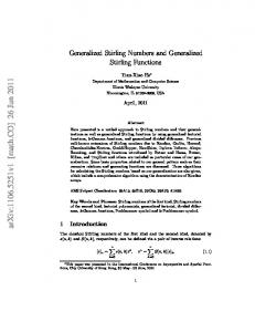
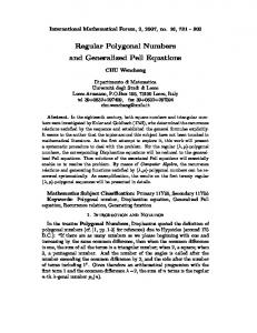
Figure 1: Examples of Cost Register Automata
2.4
CRA-definable Cost Functions
Each cost model C = (G, D, J.K) defines a class of cost functions F(C): a partial function f from Σ∗ to D belongs to this class iff there exists a CRA M over the cost grammar G such that f equals JM, CK. The class of cost functions corresponding to the cost model C(N, +) is abbreviated as F(N, +), the class corresponding to the cost model C(Q+ , +c, [0, 1], ∗d) as F(Q+ , +c, [0, 1], ∗d), etc.
2.5
Examples
Figure 1 shows examples of cost register automata for Σ = {a, b, c}. Consider the cost function f1 that maps a string w to the length of the substring obtained by deleting all b’s after the last occurrence of c in w. The automaton M1 computes this function using two cost registers and increment operation. The register y is incremented on each symbol, and hence equals the length of string processed so far. The register x is not incremented on b symbols, but is updated to the total length stored in y when c symbol is encountered. This example illustrates the use of two registers: the computation of the desired function f1 in register x update crucially relies on the auxiliary register y. For a string w and symbol a, let |w|a denote the count of a symbols in w. For a given string w of the form w1 c w2 . . . c wn−1 c wn , where each block wi contains only a’s and b’s, let f2 (w) be the minimum of the set {|wn−1 |a , |wn−1 |b , |wn |a , |wn |b }. The CRA M2 over the grammar G(min, +c) computes this function using three registers by an explicit application of the min operator. For a given string w = w1 c w2 c . . . c wn , where each wi contains only a’s and b’s, consider the function f3 that maps w to minkj=1 (|w1 |a + |w2 |a + · · · |wj |a + |wj+1 |b + · · · + |wn |b ). This function is computed by the CRA M3 over the grammar G(min, +c). The final example concerns use of scaling. Consider a computation where we wish to charge a cost of 10 upon seeing an a event until a b event occurs. Once a b event is triggered, for every subsequent c event, the cost is discounted by 5%. Such a cost function is computed by the CRA M4 over the grammar G(+c, ∗d).
2.6
Copyless Restriction
A CRA M is said to be copyless if each register is used at most once at every step: for each state q and input symbol a and each register x ∈ X, the register x appears at most once in the set of expressions {δ(q, a, y) | y ∈ X} and x appears at most once in the output expression µ(q). Each cost model C = (G, D, J.K) then defines another class of cost functions Fc (C): a partial function f from Σ∗ to D belongs to this class iff there exists a copyless CRA M over the cost grammar G such that f equals JM, CK. In Figure 1, the automata for function f2 and f4 are copyless, while the ones for f1 and f3 are not.
4
b(a|b)∗ c(a|b|c)∗ / x := x + 1 (a|c)(a|b|c)∗ / x := x + 1
q0 b(a|b)∗ / x := x µ(q0 ) = x
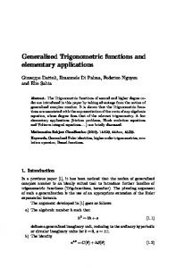
Figure 2: CRA-RLA over (+c) corresponding to M1 in Figure 1
2.7
Regular Look-Ahead
A CRA M R with regular look-ahead (CRA-RLA) is a CRA that can make its decisions based on whether the remaining suffix of the input word belongs to a regular language. Let L be a regular language, and let A be a DFA for reverse(L) (such an DFA exists, since regular languages are closed under the reverse operation). Then, while processing an input word, testing whether the suffix aj . . . ak belongs to L corresponds to testing whether the state of A after processing ak . . . aj is an accepting state of A. We now try to formalize this concept Let w = a1 . . . ak be a word over Σ∗ , and let A be a DFA with states R processing words over Σ∗ . Then the A-look-ahead labeling of w, is the word wA = r1 r2 . . . rk over the alphabet R such that for each position 1 ≤ j ≤ k, the corresponding symbol is the state of the DFA A after reading ak . . . aj (it reads the reverse of the word). A CRA-RLA consists of an DFA A over Σ∗ with states R, and a CRA M over the input alphabet R. The output of CRA − RLA (M, A) on w, denoted by J(M, A), CK(w), is defined as JM, CK(wA ). In Figure 2 we show the CRA-RLA for M1 of Figure 1.
3
Regular Cost Functions
Consider a cost grammar G = (F, T ). The terms in T can be viewed as trees: an internal node is labeled with a function symbol f of arity k > 0 and has k children, and each leaf is labeled with a constant. A deterministic-string-to-tree transduction is a (partial) function f : Σ∗ 7→ T . The theory of such transductions has been well studied, and in particular, the class of regular string-to-tree transductions has appealing closure properties, and multiple characterizations using Macro-tree-transducers (with single-use restriction and regular look-ahead) [16], Monadic-Second-Order logic definable graph transformations [11], and streaming tree transducers [3]. We first briefly recap the model of streaming tree transducers.
3.1
Streaming Tree Transducers (STT)
Streaming tree transducer is a deterministic machine model that can compute all regular transformations from ranked/unranked trees to ranked/unranked trees in a single pass. For our purpose, it suffices to restrict attention to STTs that map strings to ranked trees. The model can be viewed as a variant of cost register automata 1 , where each register stores a term, that is, an uninterpreted expression, and these terms are combined using the rules allowed by the grammar. To obtain a model whose expressiveness coincides with the regular transductions, we must require that the updates are copyless, but need to allow terms that contain “holes” or parameters that can be substituted by other terms. Let G = (F, T ) be a cost grammar. Let ? be a 0-ary special symbol that denotes a place holder for the term to be substituted later. We obtain the set T ? by adding the symbol ? to F , and requiring that each term has at most one leaf labeled with ?. For example, for the cost grammar G(+c), the set T ? of parameterized terms is defined by the grammar t := +(t, c) | c | ?; and for the cost grammar G(+), the set T ? of parameterized terms is defined by the grammar t′ := +(t, t′ ) | + (t′ , t) | c | ?, where t stands for (complete) 1 To make the definition connection precise, we need to allow registers in CRAs to be typed, and use function symbols with typed signatures. For simplicity of presentation, we defer this detail to a later version.
5
terms generated by the original grammar t := +(t, t) | c. A parameterized term such as min(5, ? + 3) stands for an incomplete expression, where the parameter ? can be replaced by another term to complete the expression. Registers of an STT hold parameterized terms. The expressions used to update the registers at every step are given by the cost grammar, with an additional rule for substitution: given a parameterized expression e and another expression e′ , the expression e[e′ ] is obtained by substituting the sole ?-labeled leaf in e with the expression e′ . Given a set X of registers, the set E ? (G, X) represents parameterized expressions that can be obtained using the rules of G, registers in X, and substitution. For example, for the grammar G(+c) and a set X of registers, the set E ? (+c, X) is defined by the grammar e := +(e, c) | c | ? | x | e[e], for x ∈ X. The output of an STT is a (complete) term in T defined using the final cost function. The variable update function and the final cost function are required to be copyless: each register is used at most once on the right-hand-side in any transition. Note that if we view an STT as a cost register automaton, then the interpretation is the identity. The semantics of an STT gives a partial function from Σ∗ to T . We refer the reader to [3] for details.
3.2
Regular Cost Functions
Let Σ be a finite input alphabet. Let D be a cost domain. A cost function f maps strings in Σ∗ to elements of D. Let C = (G, D, J.K) be a cost model. A cost function f is said to be regular with respect to the cost model C if there exists a regular string-to-tree transduction f ′ from Σ∗ to T such that for all w ∈ Σ∗ , f (w) = Jf ′ (w)K. That is, given a cost model, we can define a cost function using STTs: the STT maps the input string to a term, and then we evaluate the term according to the interpretation given by the cost model. The cost functions obtained in this manner are the regular functions. We use R(C) to denote the class of cost functions regular with respect to the cost model C. As an example, suppose Σ = {a, b}. Consider a vocabulary with constant symbols 0, ca and cb , and the grammar G(+c). Consider the STT U with a single register that is initialized to 0, and at every step, it updates x to +(x, ca ) on input a, and +(x, cb ) on input b. Given input w1 . . . wn , the STT generates the term e = +(· · · + (+(0, c1 ), c2 ) · · · cn ), where each ci = ca if wi = a and ci = cb otherwise. To obtain the corresponding cost function, we need a cost model that interprets the constants and the function symbol +, and we get the cost of the input string by evaluating the expression e. Now, consider another STT U ′ that also uses a single register initialized to ?. At every step, it updates x to x[+(?, ca )] on input a, and x[+(?, cb )] on input b, using the substitution operation. The output is the term x[0] obtained by replacing the parameter by 0. Given input w1 . . . wn , the STT generates the term e′ = +(· · · + (0, cn ), · · · c1 ), where each ci = ca if wi = a and ci = cb otherwise. Note that the STT U builds the cost term by adding costs on the right, while the STT U ′ uses parameter substitution to build costs terms in the reverse order. If the interpretation of the function + is not commutative, then these two mechanisms allow to compute different functions, both of which are regular.
3.3
Closure Properties
If f is a regular cost function from Σ∗ to a cost domain D, then the domain of f , that is, the set of strings w such that f (w) is defined, is a regular language. This follows from the properties of regular transductions. The closure properties of the class of regular string-to-tree transductions immediately imply some closure properties for regular cost functions. For a string w, let wr denote the reverse string. For a function f : Σ∗ 7→ D, the reverse function f r : Σ∗ 7→ D is defined such that for all w ∈ Σ∗ , f r (w) = f (wr ). The class of regular cost functions is closed under this operation. This is because given an STT U , we can construct an STT U r such that U r maps an input string w to the term U (wr ). Given cost functions f1 , f2 from Σ∗ to D and a language L ⊆ Σ∗ , the choice function “if L then f1 else f2 ” maps an input string w to f1 (w) if w ∈ L, and to f2 (w) otherwise. If the two cost functions f1 and f2 are regular and the condition L is a regular language, then regularity of the choice function follows. Theorem 1 (Closure Properties of Regular Cost Functions) For every cost model C, if a cost function f belongs to the class R(C), then so does the function f r ; and if two cost functions f1 and f2 belong to 6
the class R(C), then so does the function “if L then f1 else f2 ” for every regular language L. STT are also closed under the operation of regular look-ahead [2] and so regular cost functions. As we defined earlier a regular look ahead test allows a machine to make its decisions based on whether the remaining suffix of the input word belongs to a given regular language. So an STT with regular look ahead is a pair (U, A) where U is an STT and A a DFA. The function it defines is defined in the same way as that of CRA-RLA. Theorem 2 (Closure Under RLA) For every cost model STT with regular look-ahead (U, A), there exists an STT U ′ without regular look-ahead which computes the same function.
3.4
Constant Width and Linear Size of Output Terms
When an STT U computes the output term corresponding to an input string w, while processing each symbol of w, it uses exactly one transition with copyless update, and thus, the sum of the sizes of all terms stored in registers grows only by a constant additive factor. It follows that |U (w)| is O(|w|). Viewed as a tree, the depth of U (w) can be linear in the length of w, but its width is constant, bounded by the number of registers. This implies that if f is a cost function in R(N, +c), then |f (w)| must be O(|w|), and in particular, the function f (w) = |w|2 is not regular in this cost model. Revisiting the examples in Section 2, it turns out that the function f1 is regular for C(N, +c), and the function f2 is regular for C(N, min, +c). The function f3 does not appear to be regular for C(N, min, +c), as it seems to require O(|w|2 ) terms to construct it.
4
Commutative-Monoid Cost Functions
In this section we explore and analyze cost functions for the cost models of the form (D, ⊗), where D is a cost domain (with a designated identity element) and the interpretation J⊗K is a commutative and associative function.
4.1
Expressiveness
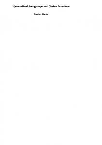
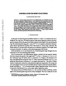
Given a cost model (D, ⊗), we can use regular string-to-term transductions to define two (machine-independent) classes of functions: the class R(D, ⊗c) defined via the grammar G(⊗c) and the class R(D, ⊗) defined via the grammar G(⊗). Relying of commutativity and associativity, we show these two classes to be equally expressive. This class of “regular additive cost functions” corresponds exactly to functions computed by CRAs with increment operation, and also, by copyless-CRAs with addition. We are going to show the result via intermediate results. Lemma 3 (R(D, ⊗c) = R(D, ⊗)) For cost domain D with a commutative associative operation ⊗, R(D, ⊗c) = R(D, ⊗). Proof. The ⊆ direction is trivial. Given an STT U from Σ∗ to G(⊗) we notice that we can construct an STT U ′ from G(⊗) to G(⊗c) that exploit the associativity of plus and creates a left parse tree where all the ⊗ nodes have a constant as right child. The basic idea is that of creating a tree to tree transducer that reads the a tree over G(⊗) and transforms it into an equivalent tree over the grammar G(⊗c). We can compute the transformation ”bottom-up”. Reading the input tree, every time we read a h+ symbol we store on the stack the tree we have computed so far as a variable z with parameter. The invariant is that every time we end processing a subtree the variable x contains the correct translation of that subtree and a parameter hole. So when we process the next subtree we can store x on the stack (as z) and at the end update x := z[x]. In the same way we update at a return +i. Now since STT are closed under composition we are done because we have that the composition of U and U ′ is an STT and precisely the one we want. � Lemma 4 (F(D, ⊗c) ⊆ R(D, ⊗c)) For cost domain D with a commutative associative operation ⊗, F(D, ⊗c) ⊆ R(D, ⊗c). 7
Proof. The fundamental property of CRA over (D, ⊗c) is that at every point at most one variable is going to contribute to the output. To see this let’s observe that our machine is deterministic and then can reach on a given string only one state. Moreover the output of a state can mention only one variable. Let’s use this as the base case of an induction argument. If at state q we can reach a state q1 with a string wa and in q1 only one variable can contribute to the final output than at the state q2 such that δ(q2 , a) = q1 we want to show that only one variable can contribute to the final output. Again our function are unary, so if for example the variable x is the one contributing to the output in q1 , the only variable that can contribute to the output in q2 is the variable y such that ρ(q2 , a, x) = f (y). So given M = (Σ, Q, q0 , X, δ, ρ, µ) we construct a RLA automaton to check which variable contribute to the output so that we only need one variable. We define for every variable x the regular language Rx such that at a state q, a ∈ Rx if starting in state q and reading a the contributing variable is x. Then assuming we are in state q, Rx = (Σ, Q × X, (q, x), Qf , δR ) where: δR ((q1 , x), a) = (q2 , x′ ) if δ(q1 , a) = q2 and ρ(q1 , a, x′ ) = f (x) and Qf = {(q ′ , x′ )|µ(q ′ ) = f (x′ )}. Since only one variable will contribute to the output the languages are disjoint. We have to create a special language Rr in the case of resets but the construction is similar. Now we only have to update the weight consistently and use the fact that STT are closed under RLA. � Lemma 5 (Fc (D, ⊗) ⊆ F(D, ⊗c)) For cost domain D with a commutative associative operation ⊗, Fc (D, ⊗) ⊆ F(D, ⊗c). Proof. We exploit the fact that in a copyless machine at every point a particular subset of variables is going to contribute to the final output. So we just compute a copy of the answer for every possible subset and we output the correct one at the end. Given a CRA M = (Σ, Q, q0 , X, δ, ρ, µ) over (D, ⊗) we construct M ′ over (D, ⊗c) in the following way: for every subset of variables S ∈ X we create a variable xS . The invariant is that every variable at every point contain the sum of the variable of its subset. Now at every update we do the following: x := x + c: ∀S.x ∈ S.xS := xS + c. hx, yi := hy, xi: ∀S.x, y ∈ S.xS := xS , ∀S.y 6∈ S ∧ S = S1 ∪ {x}.xS := xS1 ∪{y} , ∀S.x 6∈ S ∧ S = S1 ∪ {y}.xS := xS1 ∪{x} , x := c: ∀S.x ∈ S.xS := xS\{x} + c. hx, yi := hx + y, 0i: ∀S.x, y ∈ S.xS := xS , ∀S.x ∈ S, y 6∈ S.xS := xS∪{y} ∀S.y ∈ S, x 6∈ S.xS := xS\{y} . See Fig. 3 for an example of the construction. Lemma 6 (R(D, ⊗c) ⊆ F(D, ⊗)) For cost domain D with a commutative associative operation ⊗, R(D, ⊗c) ⊆ F(D, ⊗c). Proof. For the inclusion of R(D, ⊗c) in Fc (D, ⊗), observe that the parameter substitution in a unary tree can be simulated by a normal assignment for a commutative operator (e[c] is equivalent to ⊗(e, c)). So in the CRA we maintain the same set of variables and states of the STT and we only change all the substitutions to normal sum. Since the translation is copyless we are done. � Theorem 7 (Expressiveness of Additive Cost Functions) For cost domain D with a commutative associative operation ⊗, F(D, ⊗c) = Fc (D, ⊗) = R(D, ⊗c) = R(D, ⊗). Proof. Follows from Lemma 3,4,5 and 6. � We can also establish the following results regarding expressiveness of different classes. First we show that requiring CRAs with only increment is too limiting. Theorem 8 (F(D, ⊗c) * Fc (D, ⊗c)) There exists a CRA M over (D, ⊗c) that can’t be expressed as a copyless CRA M over (D, ⊗c).
8
a
a
,
x := x y := y+1 z := z
q0
b
,
,
c
,
x{x} := x{x} x{y} := x{y}+1 x{z} := x{z} x{x,y} := x{x,y}+1 x{y,z} := x{y,z}+1 x{x,z} := x{x,z} x{x,y,z}:= x{x,y,z}+1
x := x+y+z y := 0 z := 0
q0
x := x y := y z := z+1
b
,
c
,
x{x} := x{x,y,z}+1 x{y} := 0 x{z} := 0 x{x,y} := x{x,y,z}+1 x{y,z} := 0 x{x,z} := x{x,y,z}+1 x{x,y,z}:= x{x,y,z}+1
x{x} := x{x} x{y} := x{y} x{z} := x{z}+1 x{x,y} := x{x,y} x{y,z} := x{y,z}+1 x{x,z} := x{x,z}+1 x{x,y,z}:= x{x,y,z}+1
µ(q0 ) = x+y+z
µ(q0 ) = xx,y
(a) CRA (+)
(b) Corresponding CRA (+c)
Figure 3: Translation from CRA (+) to CRA (+c) Proof. We prove it using a pumping argument. We take as a counterexample the one on the left of Fig. 1. Suppose M is a copyless CRA over (D, ⊗c) that computes this function. Without loss of generality we can assume that in every assignments of the form x := y + c, y must be equal to x (if the original F(D, ⊗c) is doing some copyless renaming, we can remember the renaming in state). Now consider a string of the form bn acbn ac... where n exceeds the number of states of A. Each block of bn then must contain a cycle. Let xi be the output variable after reading (bn ac)i bn a. Now we claim that all xi ’s must be distinct because pumping in i-th block’s cycle should not change the value of xi but should change the value of all xj ’s for j > i. If A has k variables and more than k blocks, we get contradiction if the string has more than k (i.e. more than k c’s) blocks. � Second, removing the copyless restriction from CRAs with addition is too permissive as it would allow computing cost functions that grow exponentially. Theorem 9 (F(D, ⊗) * Fc (D, ⊗)) There exists a CRA M over (D, ⊗) that can’t be expressed as a copyless CRA M over (D, ⊗). Proof. The proof follows from the fundamental property of STT that states that an STT can only compute output that linearly bounded on the size of the input. This property clearly applies to Fc (D, ⊗) since we proved them to be regular. Now observe that we can create a CRA M over (D, ⊗) over the alphabet {a} such that on the first a it updates x := 2 and on the next as it updates x := x + x. Given w ∈ a∗ , the function computed is 2|w| . Clearly this can’t be expressed as a copyless-CRA. � Third, having multiple registers is essential for expressive completeness. Theorem 10 For every k ∈ N, there is a cost function f so that every CRA M over F(N, +c) has at least k variables. Proof. For each k, consider the function fk : N → N defined as fk (x) = ((x mod k) + 1) x. The input x is expressed in a unary alphabet Σ = {1}. This function outputs one of x, 2x, 3x, . . . , kx, depending on the length of x. First off, these functions can be implemented by an CRA (Fig. 4). We keep k variables v1 , . . . , vk , all initialized to 0. There are k states - q0 , . . . , qk−1 . There is a transition from qi to q(i+1) mod k , for each i. Each transition updates vi := vi + i. In state qi , we output variable vi+1 . 9
q0
q1
v1
v2
...
qi
...
qk−1 vk
vi+1
Figure 4: CRA Mk implementing fk . Each transition performs vi := vi + i, for all i. ...
... m ≥ 0 states ... n ≥ 1 states Figure 5: The structure of a possible k − 1-variable CRA M implementing fk . We now show that at least k variables are necessary. Consider otherwise, and say we are able to produce such an CRA M with k − 1 variables. The main idea is that the difference between any two “sub”-functions ax and bx, a 6= b, grows without bound. Since M works over a unary input alphabet, the only form it can assume is of a sequence of states eventually looping back to somewhere within itself (Fig. 5). Say there are m ≥ 0 states in the initial approach to the loop, and n ≥ 1 states in a single pass of the loop. Without loss of generality, assume that no variable renaming occurs. Any variable renaming information can be maintained as part of the state. Observe that no state that ever gets reset during the loop can contribute to the output afterwards, for then the output of that variable is bounded (and fk grows without bound). Consider some state q occurring in the loop, and say we our output depends on variable vi in this state. Look at the set of variables Svi = {vj } influenced by vi some p < k transitions from q. We call the pair (q, vi ) good if vi ∈ Svi . At least one good pair (q, vi ) has to exist. Now look at all constants that appear in the description of M , and pick the constant c greatest in magnitude. Then if vi comes back to the output p < k steps after q at some state q ′ , then the output in q and q ′ can differ by no more than (p + 2) |c|. But we know that for x ≥ (p + 2) |c|, the sub-functions differ by more than this amount. The contradiction is complete. � We now prove some closure properties of the model. Theorem 11 (Addition) Given two CRAs M1 and M2 over the cost model (Q, +), there exists a M over the same cost model such that ∀w ∈ Σ∗ . M (w) = M1 (w) + M2 (w). Proof. Given Mi = (Σ, Qi , q0 i , Xi , δi , ρi , µi ) (where i ∈ {1, 2}) we construct M = (Σ, Q1 ×Q2 , (q0 1 , q0 2 ), X1 × X2 , δ, ρ, µ). We want to use the variables in the following way: at every point of the computation a variable (x, y) contains the current value of x plus the current value of y. So we define: given (v1 , v2 ) ∈ Q1 × Q2 , a ∈ Σ, (x1 , x2 ) ∈ X1 × X2 , δ((v1 , v2 ), a) = (δ1 (v1 , a), δ2 (v2 , a)), ρ((v1 , v2 ), a, (x1 , x2 )) = enc(ρ1 (v1 , a, x1 ) + ρ2 (v1 , a, x2 )) where enc is the function that given the expression in the form x + y + 5 transform it into 10
(x, y) + 5 where (x, y) is the variable encoding (x + y). A technicality arises here: we actually need the set of variables to be X1 × X2 ∪ X1 ∪ X2 because assignments can be in the form x := 5, y := y + 2 and in this case the combined assignment would be x + y := y + 7 that would make us update our variable in the following way (x, y) = y + 7. It is important to notice that at most 2 variables at every point can appear in the combined right-hand side. The output function can be defined in the same way. It’s easy to see now that M computes the right function. � Theorem 12 (Subtraction) Given two CRAs M1 and M2 over the cost model (Q, +), there exists a M over the same cost model such that ∀w ∈ Σ∗ . M (w) = M1 (w) − M2 (w). Proof. Same as before. �
4.2
Weighted Automata
Weighted automaton [13] over an input alphabet Σ and a cost domain D is a nondeterministic finite-state automaton whose edges are labeled with input symbols in Σ and costs in D. For an input string w, the automaton can have multiple accepting paths from its initial state to an accepting state. The semantics of the automaton is defined using two binary functions ⊕ and ⊗ such that ⊕ is associative and commutative, and ⊗ distributes over ⊕ (to be precise, form a semiring algebraic structure). The cost of a path is the sum of the costs of all the transitions along the path according to ⊗, and the cost of a string w is obtained by applying ⊕ to the set of costs of all accepting paths of the automaton over w. Formally the weights are elements of a semiring (S, ⊕, ⊗, ¯0, ¯1). The following gives a formal definition of weighted automata. A wa from an input alphabet Σ into a set S is a tuple W = (Σ, P, I, F, E, λ, ρ) where Σ is a finite input alphabet, P is a finite set of states, I ⊆ P the set of initial states, F ⊆ P the set of final states, E a finite multiset of transitions, which are elements of P × Σ × S? × P , λ : I 7→ S an initial weight function, and ρ : F 7→ S a final weight function mapping F to S. A path π of a wa is an element of E ∗ with consecutive transitions. We denote by p[π] its origin or previous state and by n[π] its destination or next state. All the paths starting in λ and ending in ρ are called accepting. The weight of a path π, denoted w[π], is obtained by ⊗-multiplying (an operation over S) the weights of its transition. Given a string s ∈ Σ∗ , we denote by P (s) the set of accepting path over s and the weight T (s) of the string is defined as: M λ(p[π]) ⊗ w[π] ⊗ ρ(n[π]) T (s) = π∈P (s)
where ⊕ is also an operation over S. A weighted automaton is called single valued if each input string has at most one accepting path. To interpret single-valued weighted automata, we need only the interpretation for ⊗, and thus we can compare the class of functions definable by such automata with regular additive functions. Theorem 13 (Single-valued Weighted Automata) A cost function f : Σ∗ 7→ D is in R(D, ⊗c) iff it is definable by a single-valued weighted automaton Proof. We prove that for every single-valued weighted automaton W , we can construct an STT U that constructs the cost term corresponding to the sum of costs along the accepting path. Even though the automaton W is nondeterministic, since it is single-valued, the STT can use regular-look-ahead to choose deterministically the next transition that contributes to the accepting path. The proof then relies on the closure under regular-look-ahead for STTs. In the other direction, consider a CRA M using increments. At every step, the weighted automaton needs to guess which register of the machine M will contribute to the final output. The states of the weighted automaton are pairs (q, x) where q is a state in M and x is a register. There is a transition of cost k and label a from (q, x) to (q ′ , x′ ) to simulate the update: x′ := ⊗(x, k) on the a-labeled transition from q to q ′ . Clearly, since only one variable contributes to the output, the weighted automaton is single valued. An example of the translation of the function M1 of Figure 1 is in Figure 6. � 11
a, +1
0
(q0 , x)
0 c, +1
a, +1
(q0 , y)
c, +1
b, +1
b, 0 Out((q0 , x)) = 0 Out((q0 , y)) = ∞
Figure 6: Weighted Automaton corresponding to M1 in Figure 1 b
�
x := x y := y+1
q1
b
�
x := x y := y+1
q0
1 x+ � x := y = y: a a
� a x y : := x+ = y 1
�
x := x+1 y := y
q2 µ(q0 ) = x+y µ(q1 ) = x µ(q2 ) = y b
�
x := x y := y+1
Figure 7: Example CRA over (⊗) needing less variables than CRA over (⊗c)
4.3
Decision Problems
Minimum Costs The shortest path problem for CRAs is to find a string w whose cost is the minimum. For numerical domain with addition, for CRAs with increment, we can solve the shortest path problem by reducing it to classical shortest paths using the translation from CRAs with increment to single-valued weighted automata used in the proof of Theorem 13. If the CRA has n states and k registers, the graph has n · k vertices. The exact complexity depends on the weights used: for example, if the costs are nonnegative, we can use Dijkstra’s algorithm. Theorem 14 (Shortest Paths for CRAs with Inc) Given a CRA M over the cost model (Q, +c), computing min{M (w) | w ∈ Σ∗ } is solvable in Ptime. Proof. We reduce the problem to shortest path over a graph. Using the construction of Theorem 13 we create a weighted graph. The graph has |Q||X| nodes and |Σ||Q||X| edges. If the weights are all positive we can use Dijkstra algorithm with a final complexity of O(|Σ||Q||X| + |Q||X|log|Q||X|) otherwise we will use Bellman-Ford algorithm with a final complexity of O(|Q|2 |X|2 log|Q||X|). � Even though F(D, ⊗c) = Fc (D, ⊗), the model with addition can be more succinct (see Fig. 7 for an example). To solve minimum-cost problem for copyless-CRAs over the cost model (D, ⊗), we can use the translation to CRAs over (D, ⊗c) used in the proof of Theorem 7, which causes a blow-up exponential in the number of registers. We can establish an NP-hardness bound for the min-cost problem by a simple reduction from 3SAT.
12
Theorem 15 (Shortest Paths for CRAs with Addition) Given a copyless-CRA M over the cost model (Q, +) with n states and k registers, computing min{M (w) | w ∈ Σ∗ } is solvable in time polynomial in n and exponential in k. Given a CRA M over the cost model (N, +) and a constant K ∈ N, deciding whether there exists a string w such that M (w) ≤ K is np-hard. Proof. The first result follows from the complexity of the translation in Lemma 5. For the second part we give a reduction from 3-SAT. Given an instance V = {v1 , . . . , vn }, C = {c1 , . . . , ck } where V is the set of literals and C the set of clauses we create the following Fc (N, +) M . The final machine is a DAG. The machine has 2n + 1 states and k variables. The first transition simply sets all the variables to 1. The next n transition we perform different updates based on whether we decide to assign 0 or 1 to a variable. For example, in the transition from node 1 to node 2 with label 0, we set to 0 all the variables xi such that the clause ci becomes true if the variable v1 is set to false. In the last n − 1 transition we sum in a variable the values of all the variables. If this value is 0 then we have an instance for SAT, if the value is greater than 0 we don’t. This means that solving shortest path for Fc (N, +) is equivalent to solve 3-SAT. � Equivalence and Containment Given two cost register automata using addition over a numerical domain, checking whether they define exactly the same function is solvable in polynomial time relying on properties of systems of linear equations. Theorem 16 (Equivalence of CRAs with Addition) Given two CRAs M1 and M2 over the cost model (Q, +), deciding whether for all w, M1 (w) = M2 (w) is solvable in Ptime. Proof. We first take the product M = M1 × M2 . We want to check if along every path of the product, and for every final state (v1 , v2 ), if the equation µ1 (v1 ) = µ2 (v2 ) holds. The algorithm propagates such an equation over the register values backwards along each transition: for an edge from u to v, every equation e1 = e2 that must hold at v yields an equation e′1 = e′2 that must hold at u, where the expressions e′1 and e′2 are obtained from e1 and e2 using substitution to account for the update of registers along the edge from u to v. At every step of the back propagation, we maintain the basis of the set of equations in every state using Gaussian elimination. If we reach a system of equations with no solution the two machines are inequivalent, while if we reach a fix point where no independent equations can be added, the two machines are equivalent. As shown in [26], such a propagation terminates in O(nk 3 ) where n is the size of the machine (in our case |Q1 ||Q2 ||Σ|) and k is the number of variables (in our case |X 1 | + |X 2 |). Algorithm 1 Equivalence Algorithm for all v ∈ Q do G[v] = ∅ end for G[st] = {0, y = z} W = {(st, 0), (st, y = z)} while W 6= ∅ do (u, x) = Extract(W ) for all s, v such that s = ρ(u, v) do t = JsKx if t 6∈ af f (G[v]) then G[v] = G[v] ∪ {t} W = W ∪ {(v, t)} end if end for end while �
13
For CRAs that use only increment, the cubic complexity of the Gaussian elimination in the inner loop of the equivalence check can be simplified to quadratic: at every step in the back propagation, all equations are of the form x = y + c. The final complexity is O(|Q1 ||Q2 ||Σ|(|X 1 | + |X 2 |)2 ) if we only have increments and O(|Q1 ||Q2 ||Σ|(|X 1 | + |X 2 |)3 ) otherwise. � We now show that general containment is also decidable in polynomial time and that checking if a number is in the range of a CRA over (Z, +) is decidable in polynomial time. Theorem 17 (M1 ≤ M2 ) Given two CRAs M1 and M2 over the cost model (Q, +), deciding whether ∀w ∈ Σ∗ .M1 (w) ≤ M2 (w) it is in Ptime. Proof. We reduce the problem to shortest path. We in fact have that if ∀w ∈ Σ∗ .M1 (w) ≤ M2 (w) then ∀w ∈ Σ∗ .M1 (w) − M2 (w) ≥ 0. But from Theorem 12 we have a polynomial size M which is equivalent to M1 (w) − M2 (w). So we only have to solve shortest path on it and we are done. The algorithm is clearly polynomial. � Theorem 18 (k ∈ Range) Given two CRAs M over the cost model (Z, +) and a constant K ∈ Z,, deciding whether ∃w ∈ Σ∗ .M (w) = K it is in NLogSpace. Proof. We reduce the problem to 0 reachability in a weighted graph. We first compute M − c so that we now we want ∃w ∈ Σ∗ .M (w) = 0. Now we can create the same graph of shortest path and look for a 0 path on it. The problem is known to be in NLogSpace. �
5
Semiring Cost Models
In this section, we consider the cost models which result when the cost model supports two binary operations, ⊕ and ⊗, that impose a semiring structure. This structure has been studied extensively in the literature on weighted automata and rational power series. A specific case of interest is the tropical semiring, where the cost domain is N ∪ {∞}, ⊕ is the min operation, and ⊗ is arithmetic addition. While choosing a grammar, we can restrict either or both of ⊕ and ⊗ to be “unary” (that is, the second argument is a constant). To study the tropical semiring, it makes sense to choose min to be binary, while addition to be unary. Hence, in this section, we will focus on the grammar G(⊕, ⊗c), and the class R(D, ⊕, ⊗c) of cost functions.
5.1
CRA Models
Our first task is to find a suitable set of operations for cost register automata so as to have expressiveness same as the class R(D, ⊕, ⊗c). It turns out that (unrestricted) CRAs with ⊕ and ⊗c are too expressive, while their copyless counterparts are too restrictive. We need to enforce the copyless restriction, but allow substitution. In the proposed model, each register x has two fields ranging over values from D: (x.c, x.d). The intuitive understanding is that x represents the expression (x.d ⊗ ?) ⊕ x.c) where ? denotes the parameter. Such a pair can be viewed as the “most evaluated” form of a parameterized term in corresponding STTs. Expressions used for the update are given by the grammar e ::= (c, d) | x | e1 ⊗ e2 | e1 ⊕ d | e1 [e2 ] where x is a register, and c and d are constants. For the min-inc interpretation, the initial values are of the form (∞, 0) corresponding to the additive and multiplicative identities. We require that registers be used in a copyless manner, so that any particular register x appears in the update of at most one variable. The semantics of the operators on pairs is defined below: e1 ⊗ e2 is defined to be (e1 .c ⊕ e2 .c, e1 .d); e1 ⊕ d equals (e1 .c ⊗ d, e1 .d ⊗ d); and e1 [e2 ] is given by (e1 .c ⊕ e1 .d ⊗ e2 .c, e1 .d ⊗ e2 .d). The resulting model of CRA-definable cost functions is Fc (D × D, ⊗ , ⊕ d, [·]) ∗
Example 19 Consider strings w ∈ {a, b} , so that f (w) is the number of as between the closest pair of bs. This function is in F (D, min, +c), but not in the more restricted classes: F (D, min (·, d) , +c) and F (D, +c) cannot. In figure 8, we show a Fc (D × D, ⊗ , ⊕ , [·]) machine that can do this. 14
a/ x := x y := y ⊕ 1
a/ x := x y := y
q0
b/x := x, y := y
q1
a/ x := x y := y ⊕ 1
b/x := y, y := (∞, 0)
µ(q0 ) = (∞, ∞) µ(q1 ) = (∞, ∞) µ(q2 ) = x
q2
b/ x := x ⊗ y y := (∞, 0)
Figure 8: The Fc (D × D, ⊗ , ⊕ , [·]) machine for example 19. Expressiveness The next theorem summarizes the relationship between functions definable by different CRA models, which we prove in the rest of this section. Theorem 20 (Expressiveness of Semi-ring Cost Functions) If (D, ⊕, ⊗) forms a semiring, then Fc (D, ⊕, ⊗c) ⊂ Fc (D × D, ⊗ , ⊕ c, [·]) = R(D, ⊕, ⊗d) ⊂ F(D, ⊕, ⊗c) Lemma 21 If (D, ⊕, ⊗) forms a semiring, then Fc (D, ⊕, ⊗c) ⊂ Fc (D × D, ⊗ , ⊕ c, [·]) Proof. 1. Copyless CRAs with ⊕ and ⊗c can be simulated by copyless CRAs operating over pairs and performing ⊗ , ⊕ , and [·]. Given a Fc (D, ⊕, ⊗c) machine M1 , construct an Fc (D × D, ⊗ , ⊕ c, [·]) machine M2 with the same states, and same variables. Replace every occurrence of ⊕ and ⊗c in the update expressions to ⊗ and ⊕ c respectively. 2. To show strict containment, let (D, ⊕, ⊗) be the tropical semiring. We apply the same proof as in lemma 9. Here we enforce that each update is of the form x := min (x + c, . . .). Since the updates are copyless, if the min is over more than 1 term, some variable has to be reset. If there are no mins of this form, we can apply the addition-only lemma directly. Thus, if c is the largest constant in the machine, and the string pumped is ac σ, where σ was the string pumped in lemma 9, any reset variable is forever afterwards less than the function value. After k such resets, where k is the number of variables, the machine has to perform a copyful assignment. � The terms constructed by the STTs are in correspondence with their most evaluated versions maintained by CRAs. We therefore have: Lemma 22 If (D, ⊕, ⊗) forms a semiring, then Fc (D × D, ⊗ , ⊕ c, [·]) = R(D, ⊕, ⊗d). CRAs over (D, ⊕, ⊗c) can pre-emptively store values that are going to be eventually substituted: Lemma 23 If (D, ⊕, ⊗) forms a semiring, then R(D, ⊕, ⊗d) ⊆ F(D, ⊕, ⊗c). Proof. Consider a copyful CRA machine M over (D × D, ⊗ , ⊕ , [·]). Let Vr be the set of its variables. The goal is to construct a copyful CRA machine M ′ over (D, ⊕, ⊗c). We perform the following subset construction over variables. The states and transitions of M ′ are the same as in M . The set of variables Vl is the following: 15
1. x.c and x.d for every x ∈ Vr . 2. For every S ⊆ Vr , we maintain dS = ⊗x∈S x.d, and for all x ∈ / S, xdS = x.c ⊗ dS . The expression on the right of each of the above equalities is the intended invariant we’ll maintain. Because of the properties of the semiring, we can simplify the resulting expression into a linear form. We define an elementary update in M as one in which: the value of no variable changes, or exactly two variables permute: hx, yi := hy, xi, or exactly one variable is reset: x := (c, d), or exactly one variable changes: x := x ⊕ d, or exactly two variables change (addition): hx, yi := hx ⊗ y, (0, 1)i, or exactly two variables change (substitution): hx, yi := hx [y] , (0, 1)i. Observe that any copyless variable update can be written as a finite sequence of elementary updates. Also a finite sequence of updates in a CRA machine over (D, ⊕, ⊗c) can be summarized into a single update. Thus, if we demonstrate a semantics-preserving transformation from elementary updates to copyful linear updates, we are done. Given a variable x ∈ Vl , let x be its value before the update, and x′ be its intended value after. We show that x′ in each case can be written as a linear combination of the old values, thus giving a linear update rule x := Expr. Only the last two cases are interesting: 1. Addition: hx, yi := hx ⊗ y, (0, 1)i. (a) x.c′ = x.c ⊕ y.c, x.d′ = x.d. y.c′ = 0 and y.d′ = 1. (b) For z 6= x, y. z.c′ = z.c and z.d′ = z.d. (c) For S, x, y ∈ / S. d′S = dS , xd′S = (x.c ⊕ y.c) ⊗ d′S = xd′S ⊕ yd′S . yd′S = 0, and zd′S = zdS . (d) For S, x ∈ S, but y ∈ / S. d′S = dS , yd′S = 0, and zd′S = zdS . (Exactly the same as the previous case.) (e) For S, x ∈ / S, but y ∈ S. Let S ′ = S \ {y}. d′S = y.d′ ⊗ d′S ′ = dS ′ . xd′S = x.c′ ⊗ d′S = (x.c ⊕ y.c) ⊗ dS ′ = xdS ′ ⊕ ydS ′ . zd′S = z.c′ ⊗ d′S = z.c ⊗ dS ′ = zdS ′ . (f) For S, x, y ∈ S. S ′ = S \ {x, y}. d′S = x.d′ ⊗ y.d′ ⊗ d′S ′ = x.d ⊗ dS ′ = dS ′ ∪{x} . zd′S = z.c′ ⊗ d′S = zdS ′ ∪{x} . 2. Substitution: hx, y := x [y] , (0, 1)i. This shows why we needed to keep the subset variables. (a) x.c′ = x.c ⊕ x.d ⊗ y.c = x.c ⊕ yd{x} . x.d′ = x.d ⊗ y.d = d{x,y} . y.c′ = 0 and y.d′ = 1. (b) For z 6= x, y, z.c′ = z.c and z.d′ = z.d. (c) For S, x, y ∈ / S. d′S = dS , xd′S = x.c′ ⊗ d′S = (x.c ⊕ x.d ⊗ y.c) ⊗ dS = xdS ⊕ ydS∪{x} . yd′S = 0, ′ and zdS = zdS . (d) For S, x ∈ S but y ∈ / S. Let S ′ = S \ {x}. d′S = x.d′ ⊗ d′S ′ = d{x,y} ⊗ dS ′ = dS∪{y} . yd′S = 0, and ′ ′ ′ zdS = z.c ⊗ dS = z.c ⊗ dS∪{y} = zdS∪{y} . � (e) x ∈ / S, but y ∈ S. Let S ′ = S \{y}. d′S = y.d′ ⊗d′S ′ = dS ′ . xd′S = x.c′ ⊗d′S = x.c ⊕ yd{x} ⊗dS ′ = xdS ′ ⊕ ydS ′ ∪{x} . zd′S = z.c′ ⊗ d′S = z.c ⊗ dS ′ = zdS ′ . (f) Both x, y ∈ S. Let S ′ = S \ {x, y}. d′S = x.d′ ⊗ y.d′ ⊗ d′S ′ = d{x,y} ⊗ dS ′ = dS ′ ∪{x,y} = dS . zd′S = z.c′ ⊗ d′S = z.c ⊗ dS = zdS . � Finally, the containment established by the above theorem is strict. Lemma 24 Over the tropical semiring, there exist functions in F (D, ⊕, ⊗c) which are not in R(D, ⊕, ⊗d).
16
� Proof. An example of such a function is f3 in figure 1. Regardless of the string w, f wb|w| c = |w|a . Thus, in any state q, the machine has to contain, in some register xq , |w|a + cqx . However, for all w and k > 0, there is some σ so that |f (wσ) − |wσ|a | ≥ k. Let’s identify some witness for this by writing σ (w, k). In particular, this means that there has to be some register tracking the value of the function, which is distinct from the register xq tracking |w|a . We have thus established that at least two variables are necessary. Consider a machine with two variables. For the largest constant c appearing in the description of the machine, consider the string ac σ (ac , c). At this point, we have two registers - one containing the number of as, and the other containing the function. If we now feed the machine a suffix b|σ(ǫ,c)| c, the value of the function is equal to the number of as in the input string. The machine now has two choices: either copy the value, or choose to track both the function and the number of as in the same register. This latter choice � |σ(ǫ,c)| c)| c, and force the machine cannot happen: for we can then feed the suffix σ σ (ǫ, c) b|σ(ǫ,c)| c b|σ(σ(ǫ,c)b into making a mistake. For multiple variables, we perform a multi-step pumping argument similar to the above. Define the c c sequence: σ1 = ac σ (ac , c), σs = σ1 ac b|σ1 a | c, . . . , σi+1 = σi ac b|σi a | c, . . . The argument involves observing after reading each σi , the number of “useful” variables, in the absence of copyful assigments, decreases by one: σ1 σ2 . . . σi . . .. �
5.2
Relation to Weighted Automata
In Section 4, we noted that single-valued weighted automata correspond exactly to CRAs with addition. Now we show that nondeterministic weighted automata and (deterministic) CRAs (without the copyless restriction) with ⊕ and ⊗c express exactly the same class of functions. The translation from weighted automata to CRAs can be viewed as a generalization of the classical subset construction for determinization. Theorem 25 (Weighted Automata Expressiveness) If (D, ⊕, ⊗) forms a semiring, then the class of functions F (D, ⊕, ⊗c) is exactly that representable by weighted automata. Proof. Let W = (Σ, P, I, F, E, λ, ρ) be the weighted automaton. Construct the corresponding CRA M over (D, ⊕, ⊗ c): The set of states Q = 2P . The state set is obtained by the standard subset construction. The intuition is that M is in state q ⊆ P after processing a string w if it is exactly the set of states reachable in W on processing w. Thus, δ (q, a) = {p′ ∈ P | ∃p ∈ q, p →aW p′ }. The initial state q0 is the set of initial states of the weighted automaton, I. The set of registers is X = {xp | p ∈ P }: there is a register xp for every state p ∈ P . Intuitively, the xp holds the ⊕-sum of the ⊗-product of the weights of all paths. For each state p ∈ I, the register xp is initialized to λ (p). Observe that initial values are merely syntactic sugar - thus we use them even though we omitted them from the definition of CRAs. When the CRA makes a a,c transition q →a q ′ , the variable update is given by ∀p′ ∈ q ′ , xp′ := ⊕{xp ⊗ c | p →W p′ }. That is, to obtain the value of xp′ , we consider each state p such that there is an a-labeled transition from p to p′ with cost c in the weighted automaton, add c to xp according to ⊗, and take ⊕ over all such values. In state q ⊆ P , the output function is defined as ⊕ {xp ⊗ ρ (p) | p ∈ q}. The output function is the ⊕-sum of all the product of all paths. To prove the correctness of this construction, observe the inductive invariant: for all w, and for all states p, the register xp in the CRA M contains the ⊕-sum of the ⊗-product of the weights of all paths leading from some initial state to p on w. This depends on the distributivity of ⊗ over ⊕. Note that the same register xp contributes to all xp′ s for all its a-successor states p′ . Thus, the udpate is not necessarily copyless. In the reverse direction, let M be a CRA over (D, ⊕, ⊗ c) with states Q and registers X. Construct the following weighted automaton W : The states P = Q × X ∪ Q. A state qx ∈ Q × X calculates the transformations happening to individual variables, while states q ∈ Q are there to effect the constant offset possibly imposed by the output function. The initial states I = {q0 } × X ∪ {q0 }. The initial weights are all the multiplicative identity. Say the output function at state q ∈ Q in M is ⊕i xi ⊗ ai + cq . Then the output ′ weight ρ (q, x) = ai and ρ (q) = cq . Whenever there is a transition q →aM q ′ , there is a transition q →a,1 W q . Also, for every variable update x := ⊕i xi ⊗ ai ⊕ cx that happens during this transition, create the transition a,cx i ′ ′ (q, xi ) →a,a W (q , x) in W . Also add the transition q →W (q , x) The weighted automaton cannot apply the 17
⊕-operation locally, but it preserves all paths, and the ⊕-operation is applied to all paths leading to a final state at the end. Correctness involves establishing the invariant: after processing w, the ⊕-sum of all paths leading to some state (q, x) is the value of xq in M after processing w. This follows from the distributivity properties of a semiring. �
5.3
Decision Problems for Min-Plus Models
Now we turn our attention to semirings in which the cost domain is a numerical domain such as N ∪ {∞}, ⊕ is the minimum operation, and ⊗ is the addition. First let us consider shortest path problems for CRAs over the cost model (Q ∪ {∞}, min, +c). Given a CRA over such a cost model, we can construct a weighted automaton using the construction in the proof of Theorem 25. Shortest paths in a weighted automaton can be solved in polynomial-time using standard algorithms [24]. Theorem 26 (Shortest Paths in CRAs over min and +c) Given a CRA M over the cost model (Q ∪ {∞} , min, +c), computing min{M (w) | w ∈ Σ∗ } is solvable in Ptime. It is known that the equivalence problem for weighted automata over the tropical semiring is undecidable. It follows that checking whether two CRAs over the cost model (N ∪ {∞} , min, +c) compute the same cost function, is undecidable. The existing proofs of the undecidability of equivalence rely on the unrestricted non-deterministic nature of weighted automata, and thus on the copyful nature of CRAs with min and +c. We conjecture that the equivalence problem for copyless CRAs over (N ∪ {∞} , min, +c), and also for the class R(N ∪ {∞} , min, +c) is decidable.
6
Discounted Costs
In this section, we focus on the class of regular cost functions definable using +c and ∗d. Such cost functions allow both adding costs and scaling by discount factors.
6.1
Past Discounts
First let us focus on CRAs over the cost model C (Q, +c, ∗d). At every step, such a machine can set a register x to the value d ∗ x + c: this corresponds to discounting previously accumulated cost in x by a factor d, and paying an additional new cost c. We call such machines the past-discount CRAs (see M4 of Figure 1 for an example). Note that the use of multiple registers means that this class of cost functions is closed under regular choice and regular look-ahead: the discount factors can depend conditionally upon future events. It is easy to check that the cost functions definable by past-discount CRAs belong to the class R(Q, +c, ∗d). Our main result for past-discount CRAs is that the min-cost problem can be solved in polynomial-time. First, multiple variables can be handled by considering a graph whose vertices are pairs of the form (q, x), where q is a state of the CRA, and x is a register. Second, classical shortest path algorithm can be easily modified when the update along an edge scales the prior cost before adding a weight to it, this is sometimes called generalized shortest path (see [29]). Theorem 27 (Shortest Paths for Past Discounts) Given a past-discount CRA M over the cost model (Q, +c, ∗d), computing min{M (w) | w ∈ Σ∗ } is solvable in Ptime. Proof. We translate this problem into the generalized shortest path problem (see [29]) on a graph. For each state q in Q and each register x in X, we construct a node (q, x). Moreover, we construct an extra node (q, 0) for each q, and a source node s. For each transition δ(q, a) = q ′ in M , and each y, if ρ(q, a, y) = dx + c, d 6= 0 for some x, we create an edge e from (q ′ , y) to (q, x) , with label a and weight d,cost c; if ρ(q, a, y) = 0, we create an edge from (q ′ , y) to (q, 0), with label a and weight 0,cost 0; create an edge from (q ′ , 0) to (q, 0), with label a and weight 0,cost 0. For each q ∈ Q, if µ(q) = dx + c, d 6= 0, then create an edge from s to (q, x) with label ε and weight d,cost c; otherwise if µ(q) = c, where c is a constant, we create an edge from s 18
to (q, 0) with label ε and weight 0,cost c. Finally, we create a sink node t, and connect (q0 , x), ∀x ∈ X and (q0 , 0) to t with label ε and weight 0,cost 0. It is easy to verify that the the cost of the general shorted path on the graph is equal to the cost of the shortest path for past discount machine. �
6.2
Future Discounts
Symmetric to past discounts are future discounts: at every step, the machine wants to pay an additional new cost c, and discount all future costs by a factor d. While processing an input w1 . . . wn , if the sequence of local costs is c1 , . . . cn and discount factors is d1 , . . . dn , then the cost of the string is the value of the term (c1 + d1 ∗ (c2 + d2 ∗ (· · · ))). Future-discount CRAs are able to compute such cost functions using registers that range over Q × Q and substitution: each register holds a value of the form (c, d) where c is the accumulated cost and d is the accumulated discount factor, and updates are defined by the grammar e := (c, d)|e[c, d]|x. The interpretation for e[c, d] is defined to be (e.c + c ∗ e.d, e.d ∗ d) (that is, the current discount factor e.d is scaled by new discount d, and current cost e.c is updated by adding new cost c, scaled by the current discount factor e.d). Like past-discount CRAs,future-discount CRAs are closed under regular choice and regular look-ahead. Processing of future discounts in forward direction needs maintaining a pair consisting of cost and discount, and the accumulated costs along different paths is not totally ordered due to these two objectives. However, if we consider paths in “reverse”, a single cost value updated using assignments of the form x := d ∗ x + c as in past-discount CRAs suffices. Theorem 28 (Shortest Paths for Future Discounts) Given a future-discounted CRA M over the cost model (Q, +c, ∗d), computing min{M (w) | w ∈ Σ∗ } is solvable in Ptime. Proof. We translate this problem into the generalized shortest path problem [29] on a directed graph G. For each state q in Q and each variable x in X, we construct a node (q, x). Moreover, we construct an extra node (q, 0) for each q, and a sink node t, a source node s. For each transition δ(q, a) = q ′ in M , and each y, if ρ(q, a, y) = x[c, d] for some y, we create an edge e from (q, x) to (q ′ , y), with label a and weight d,cost c; if ρ(q, a, y) = (c, d), we create an edge from (q, 0) to (q ′ , y), with label a and weight d,cost c; create an edge from (q, 0) to (q ′ , 0) with label a and weight 1,cost 0. For each q ∈ Q, if µ(q) = x[c, d], then create an edge from (q, x) to t with label ε and weight d,cost c; otherwise if µ(q) = (c, d), we create an edge from (q, 0) to t with label ε and weight d, cost c. Finally, create an edge from s to (q0 , x), ∀x ∈ X and (q0 , 0) , with label ε and weight 1,cost 0. It is easy to verify that solving the generalized shortest path on the graph G is equivalent to solving the shortest path for future discount machine M . �
6.3
Global Discounts
A global-discount CRA is capable of scaling the global cost (the cost of the entire path) by a discount factor. As in case of future-discount CRAs, it uses registers that hold cost-discount pairs. We now assume that discounts range over [0, 1] and costs range over Q+ . The registers are updated using the grammar e := (0, 1) | e + (c, d) | x. The interpretation for e + (c, d) is defined to be (d ∗ e.c + e.d ∗ c, e.d ∗ d) (that is, the current discount factor e.d is scaled by new discount d, and current cost e.c is updated by first scaling it by the new discount, and then adding new cost c scaled by the current discount factor e.d). Analyzing paths in a global-discount CRA requires keeping track of both the accumulated cost and discount. We can show a pseudo-polynomial upper bound; it remains open whether there is a strongly polynomial algorithm for shortest paths for this model: Theorem 29 (Shortest Paths for Global Discounts) Given a global-discounted CRA M over the cost model (Q+ , +c, [0, 1], ∗d) and constant K, deciding min{M (w) | w ∈ Σ∗ } ≤ K is solvable in np. Computing the minimum is solvable in Ptime assuming increments are restricted to adding natural numbers in unary encoding. Proof. Using the state-cross-variable construction used in earlier proofs, we can reduce the min-cost problem to finding a shortest path in a graph G whose edges are labeled with (c, d) pairs, and the cost of 19
Q P a path containing edges labeled with (c1 , d0 ) · · · (cn , dn ) is ( i ci )( i di ). First, observe that if there is a reachable cycle such that the cycle contains an edge with discount factor < 1, then repeating this cycle drives the global discount to 0, and thus, existence of such a cycle implies that the (limiting) min-cost is 0. Note that the shortest path need not involve a cycle in which all discount factors are equal to 1 (since costs are non-negative). The np-bound follows. Suppose incremental costs ci ’s are small natural numbers. The pseudo-polynomial algorithm for this case relies on following: for a given value c and a vertex v, computing the “best” global discount over all paths from source to v with sum of incremental costs equal to c, can be solved by adopting shortest path algorithms, and the set of interesting choices of c can be bound by nk for a graph with n vertices if each increment is a number between 0 to k. �
6.4
Regular Functions for Inc-Scale Model
The class of regular functions for the cost model (Q, +c, ∗d) is defined via STTs over the inc-scale grammar G(+c, ∗d). It is to show that: Theorem 30 (Expressiveness of Inc-Scale Models) The cost functions definable by past-discount CRAs, by future-discount CRAs, and by global-disount CRAs all belong to R(Q, +c, ∗d). The min-cost problem for this class of functions is still open. However, we can show the equivalence problem to be decidable. First, using the construction similar to the one used to establish R(D, ⊕, ⊗c) ⊂ F(D, ⊕, ⊗c) (see Theorem 20), we can represent cost functions in R(Q, +c, ∗d) using (copyful) CRAs that use + and ∗d. Such CRAs have linear updates, and the algorithm for checking equivalence of CRAs with addition can be used for this case also. Theorem 31 Given two function f1 , f2 ∈ R(Q, +c, ∗d) represented by STTs over the cost grammar G(+c, ∗d), checking whether the two functions coincide, can be solved in time polynomial in the number of states and exponential in the number of registers. Proof. We show that given an SST T for f ∈ R(D, +C, ∗D), we can construct an equivalent machine CRA Q M using + and ∗d as following. For each subset S of registers in T , maintain dS = y∈S y.d, and for each x and S such that x 6∈ S, also maintain xS = x.c ∗ dS . We’ll translate all the updates on each transition to the linear transformation on dS and xS . Any update can be expressed as a sequence of the following updates: 1) x := (x.c + y.c, x.d) and y := (0, 1); 2) x := (x.c + x.d ∗ y.c, x.d ∗ y.d) and y := (0, 1); 3)x := (c, d). For case 1), for each subset S, if y 6∈ S, let dS := dS , xS := xS + yS , yS := 0 and zS := zS for other registers; if y ∈ S, let dS := dS\{y} , xS := xS\{y} + yS\{y} and zS := zS\{y} for other registers. For case 2), for each subset S, if x, y 6∈ S, then let dS := dS , xS := xS + yS∪{x} , yS := 0 and zS := zS for other registers; if x ∈ S, y 6∈ S, then let dS := dS∪{y} , yS := 0 and zS := zS∪{y} for other registers; if x 6∈ S, y ∈ S, then let dS := dS\{y} , xS := xS\{y} + yS\{y}∪{x} and zS := zS\{y} for other registers; if x ∈ S, y ∈ S, then let dS := dS and zS := zS for other registers. For case 3), for each subset S, if x 6∈ S, let dS := dS , xS := c ∗ dS and zS := zS for other registers; if x ∈ S, let dS := d ∗ dS\{x} and zS := d ∗ zS\{x} for other registers. Since equivalence checking between two CRAs with + and ∗d is solvable in time polynomial in the number of states and the number of registers, equivalence checking for R(D, +C, ∗D) is solvable in time polynomial in the number of states and exponential the number of registers. �
7
Related Work
Weighted Automata (wa) and Logics. Finite-state wa have been an active area of research, with numerous articles studying their algebraic and algorithmic properties. See [13] for a comprehensive exposition. wa can be viewed as classic nondeterministic finite automata in which each transitions is additionally associated with a weight. Thus, these automata define functions that map each word from their domain (which is a regular language) to some weight. The algebraic structure underlying the computation of a wa is a semiring: the binary operator ⊗ of the semiring is used to compute the weight of a path in the automaton,
20
and the ⊕ operator is used for summing the weights of the successful paths. The behaviors of a wa define a rational power series, or could be said to define rational functions. wa have desirable properties: the all-pairs shortest distance (or minimum cost flow) problem is decidable with Ptime complexity for complete semirings, and the model has closure under binary operations such as sum, difference, intersection, reversal, and inversion [24]. An important problem for wa is that of determinization [24, 22]. A deterministic wa is defined in the usual sense: no two outgoing transitions from a state share the same input label. It has been shown that there are wa that do not admit equivalent deterministic wa. In contrast, the cost register automata that we introduce in this paper are deterministic machines with equivalent expressive power and equally efficient decision problems as weighted automata. We argue that this makes them a more suitable model for expressing weighted computations. It has been shown that the equivalence problem for wa over the tropical semiring is undecidable using a reduction from Hilbert’s tenth problem [23], and by a reduction from the halting problem for two counter machines [1]. The only known class of weighted automata with decidable equivalence problem is that of finite-valued weighted automata [31]. We conjecture that the equivalence problem for CRA over min and +c with the copyless restriction is decidable. If this is true, it would give the largest known class with decidable equivalence that subsumes weighted automata. In [12], the authors discuss a weighted MSO-logic that disallows universal second order quantification and places restrictions on universal first order quantification. The authors show that the formal power series definable in this logic coincides with the set of behaviors of weighted automata. In contrast, in this paper, we introduce automata and machines that exactly capture MSO-definable cost functions. Discounted weighted computations and Generalized Shortest Paths. Generalized network flow problems extend flow problems on directed graphs by specifying multipliers on edges in addition to costs [18, 29]. The problem of finding the minimum cost flow (which in some cases is equivalent to the shortest distance path) from a source to a target can be solved in polynomial time [29, 5]. Future discount machines that we introduce in this paper provide a nice formalism that subsumes such problems, and have strongly polynomial time algorithms for determining the minimum cost path. In this paper, we also introduce past discount and global discount machines that also have efficient algorithms for determining the minimum cost paths. These machines thus have great potential to model a rich variety of discounted and weighted computations. In [14], the authors introduce weighted logic for infinite words. In order to address convergence of the weighted sum, the authors assume discounting along later edges in a path (i.e., future discounting). Extending the results of this paper to discounted weighted computations over infinite words remains open. Transducer Models. A wide variety of different models have been proposed to model string and tree transductions. The models that are most relevant to this paper are MSO-definable transductions [11, 15] and macro tree transducers [17, 16]. An MSO-definable graph transduction specifies a function between sets of graphs; the nodes, edges and labels of the output graph are described in terms of MSO formulas over the nodes, edges and labels of a finite number of copies of the input graph. A macro tree transducer (MTT) is a top-down tree to tree transducer equipped with parameters. Parameters can store temporary trees and append them to the final tree during the computation. In general, MTT are more expressive than MSOdefinable tree transductions. A subclass of MTTs obtained by restricting the number of times a subtree and a parameter can be used has been shown to be equi-expressive as MSO-definable tree transductions [16]. In addition to these models, formalisms such as attribute grammars [16], attribute tree transducers [7] have also been studied. Streaming tree transducers [3] (STTs), introduced by two of the co-authors in this paper are a new formalism for expressing MSO-definable tree-to-tree and string-to-tree transductions. In comparison to some of the transducer models discussed above, STTs have distinguishing features that make them desirable as a canonical model for specifying regular or MSO-definable transductions: (1) STTs produce the output in linear time by performing a single pass over the input, (2) they preserve desirable properties such as closure
21
under sequential composition and regular look-ahead, and (3) they have good algorithmic properties such as decidability of functional equivalence. Regularity over Data Languages. Data languages allow finite strings over data values that can be drawn from a possibly infinite data domain [28], [20] [6]. Beyond the similarity in nomenclature, register automata that are studied in this line of work are quite distinct from register cost automata, as the former are essentially defined over an infinite input alphabet. A critical difference lies in the fact that almost every variant of data automata allows testing equality of data values, which mostly causes interesting decision problems to become undecidable. Cost register automata use the cost registers in a strictly write-only fashion, which makes them incomparable to variants of data automata that use read/write registers. Regular Cost Functions. In [9], Colcombet defines a regular cost function as a mapping from words to Nω (the set of nonnegative integers and the ordinal ω). A cost function is precisely defined as an equivalence class over mappings from the set of words to Nω , such that functions f and g are in the same equivalence class if for all words w, f (w) is bounded by some constant iff g(w) is bounded is bounded by some constant. The author then defines two classes of automata (B- and S-automata), each of which uses a finite set of counters and allows the counters to be incremented, reset or checked for equality with a constant. The operational semantics of these automata are that the automaton computes the least upper bound or the greatest lower bound over the set of counter values encountered during its run. A cost function is then called regular if it is accepted by a history-deterministic B- or S-automaton. The author also provides an algebraic characterization of regular cost functions in terms of stabilization monoids and equates recognizability of cost functions with regularity. In [10], the authors extend this notion to regular cost functions over trees. It is clear that the notions proposed in this line of work are orthogonal to our characterization of regularity of cost functions. The authors state that the motivation for the work in [9, 10] is preserving nice algorithmic and closure properties of regular languages for problems such as equivalence and projection. However, the integer values in these functions are considered modulo an equivalence which preserves existence of bounds on the function values, but not the values themselves. We argue that the notion of regularity of cost functions that we propose in this paper is closer to the classical notions of regularity such as MSO-definability. Affine Programs. In [21], and more recently in [26, 27], the authors present the problem of deriving affine relationships among variables of a program. A generalization of the discounted CRA model presented in this paper is to consider automata which allow arbitrary affine transformations on the set of registers as part of their transitions. While the cost functions defined by such “affine transducers” do not have interesting regularity properties, we remark that the equivalence of such transducers can be checked in polynomial time by using ideas similar to the ones in [26]. Quantitative Languages. A quantitative language [8, 1, 4] over infinite words is a function Σω 7→ R. Such languages are generated by weighted automata, where the value of a word w is set as the maximal value of all runs over w. By defining various value functions such as M ax, Sum, LimSup, LimInf , different values can be computed for the run of a weighted automaton on the string w. Quantitative languages use the fixed syntax of weighted automata, and thereby restricted to having a single weight along each transition in their underlying automata. Moreover, they face similar difficulties in determinization: for interesting models of value functions, the corresponding automata cannot be determinized. An extension of CRA to ω-regular cost functions could prove to be a more expressive and robust model to specify quantitative languages and to analyze their decision problems.
8
Conclusions
We have proposed a new approach to define regular functions for associating costs with strings. The results for various classes of functions are summarized in Figure 2. We hope that our work provides new insights
22
CRA (⊕, ⊗c) ≡ Weighted Automata Reg (D, ⊕, ⊗c) CopylessCRA (⊕, ⊗c) Reg (D, ⊕c) ≡ Past Disc- Reg (D, ⊕) ≡ ounts CRA (⊕c) ≡ CopylessCRA (⊕) ≡ Single-valued wa Global Discounts
Future Discounts
Reg (D, ⊕c, ⊗d) ≡ CRA Inc-Scale
CRA with
Equivalence
Min-Cost
(+c) Copyless (+) (min, +c) Copyless (min, +c) Past-discounts Future-discounts Global-discounts Inc-Scale
Ptime Ptime Undecidable ?
Ptime ExpTime Ptime Ptime Ptime Ptime Pseudo-Poly ?
Poly in states Exp in registers
(b) Complexity of Decision Problems
(a) Hierarchy for CRA models
Figure 9: Summary of Results into the well-studied topic of weighted automata, and opens a whole range of new problems. First, it is plausible that there is a compelling notion of congruences and canonicity for CRAs with increment. Second, the decidability of copyless-CRAs with min and increment remains an intriguing open problem. Third, we don’t have algorithms for the min-cost problem for the class of regular functions with increment and scaling. While we have not succeeded even in establishing decidability, we suspect that this problem admits efficient approximation algorithms. Fourth, we have considered only a small set of combinations of operations; studying the effects of adding operators such as max would be worthwhile. Fifth, our notion of regularity and cost register automata for mapping strings to costs can be extended to infinite strings and trees, as well as to timed and probabilistic systems. Finally, we would like to explore practical applications: our framework seems suitable for expressing complex, yet analyzable, pricing policies, say, for power distribution.
References [1] S. Almagor, U. Boker, and O. Kupferman. Whats decidable about weighted automata? In Automated Technology for Verification and Analysis, Lecture Notes in Computer Science, pages 482–491, 2011. ˇ [2] R. Alur and P. Cern´ y. Streaming Transducers for Algorithmic Verification of Single-pass List-processing Programs. In Proc. of Principles of Programming Languages, pages 599–610, 2011. [3] R. Alur and L. D’Antoni. Streaming tree transducers. CoRR, abs/1104.2599, 2011. [4] B. Aminof, O. Kupferman, and R. Lampert. Reasoning about online algorithms with weighted automata. ACM Transactions on Algorithms, 6(2), 2010. [5] V. Batagelj, F. J. Brandenburg, P. O. D. Mendez, and A. Sen. The generalized shortest path problem. In CiteSeer Archives, 2000. [6] H. Bj¨orklund and T. Schwentick. On notions of regularity for data languages. Theor. Comput. Sci., 411(4-5):702–715, 2010. [7] R. Bloem and J. Engelfriet. A comparison of tree transductions defined by monadic second order logic and by attribute grammars. J. Comp. and Sys. Sci., 61(1):1 – 50, 2000. [8] K. Chatterjee, L. Doyen, and T. A. Henzinger. Quantitative languages. ACM Trans. Comput. Log., 11(4), 2010. [9] T. Colcombet. The theory of stabilisation monoids and regular cost functions. pages 139–150, 2009. [10] T. Colcombet and C. Loding. Regular cost functions over finite trees. In Symposium on Logic in Computer Science, pages 70–79, 2010. 23
[11] B. Courcelle. Graph Operations, Graph Transformations and Monadic Second-Order Logic: A survey. Electronic Notes in Theoretical Computer Science, 51:122 – 126, 2002. [12] M. Droste and P. Gastin. Weighted automata and weighted logics. In Proc. of International Colloquium on Automata, Languages and Programming, pages 513–525, 2005. [13] M. Droste, W. Kuich, and H. Vogler, editors. Handbook of Weighted Automata. Springer-Verlag, 2009. [14] M. Droste and G. Rahonis. Weighted automata and weighted logics with discounting. Theor. Comp. Sci., 410(37):3481 – 3494, 2009. [15] J. Engelfriet and H. J. Hoogeboom. MSO definable String Transductions and Two-way Finite-State Transducers. ACM Transactions on Computational Logic, 2(2):216–254, 2001. [16] J. Engelfriet and S. Maneth. Macro tree transducers, attribute grammars, and mso definable tree translations. Information and Computation, 154(1):34 – 91, 1999. [17] J. Engelfriet and H. Vogler. Macro tree transducers. Journal of Computer and System Sciences, 31(1):71 – 146, 1985. ´ Tardos. Combinatorial Algorithms for the Generalized Circulation [18] A. V. Goldberg, S. A. Plotkin, and E. Problem. In Foundations of Computer Science, pages 432–443, 1988. [19] H. Hosoya. Foundations of XML Processing: The Tree-Automata Approach. Cambridge University Press, 2011. [20] M. Kaminski and N. Francez. Finite-memory automata. Theor. Comput. Sci., 134(2):329–363, 1994. [21] M. Karr. Affine relationships among variables of a program. Acta Inf., 6:133–151, 1976. [22] D. Kirsten and I. M¨ aurer. On the determinization of weighted automta. J. Autom. Lang. Comb., 10:287–312, 2005. [23] D. Krob. The equality problem for rational series with multiplicities in the tropical semiring is undecidable. In International Colloquium on Automata, Languages and Programming, pages 101–112, 1992. [24] M. Mohri. Weighted Automata Algorithms. In M. Droste, W. Kuich, and H. Vogler, editors, Handbook of Weighted Automata, pages 213–254. Springer Berlin Heidelberg, 2009. [25] M. Mohri, F. Pereira, and M. Riley. Weighted finite-state transducers in speech recognition. Computer Speech & Language, 16(1):69–88, 2002. [26] M. M¨ uller-Olm and H. Seidl. A note on Karr’s algorithm. In International Colloquium on Automata, Languages and Programming, pages 1016–1028, 2004. [27] M. M¨ uller-Olm and H. Seidl. Precise interprocedural analysis through linear algebra. In Principles Of Programming Languages, pages 330–341, 2004. [28] F. Neven, T. Schwentick, and V. Vianu. Finite state machines for strings over infinite alphabets. ACM Trans. Comput. Log., 5(3):403–435, 2004. [29] J. D. Oldham. Combinatorial Approximation Algorithms for Generalized Flow Problems. In Symposium On Discrete Algorithms, pages 704–714, 1999. [30] M. P. Sch¨ utzenberger. On the definition of a family of automata. Information and Control, 4:245–270, 1961. [31] A. Weber. Finite-valued distance automata. Theor. Comput. Sci., 134:225–251, November 1994.
24