Each time stamp ti denotes the amount of time elapsed ...... [1] Parosh Aziz Abdulla, Johann Deneux, Joël Ouaknine & James Worrell (2005): Decidability and ...
Relating timed and register automata ∗ Diego Figueira
Piotr Hofman
Sławomir Lasota
INRIA, ENS Cachan, LSV France
Institute of Informatics University of Warsaw Poland
Institute of Informatics University of Warsaw Poland
Timed automata and register automata are well-known models of computation over timed and data words respectively. The former has clocks that allow to test the lapse of time between two events, whilst the latter includes registers that can store data values for later comparison. Although these two models behave in appearance differently, several decision problems have the same (un)decidability and complexity results for both models. As a prominent example, emptiness is decidable for alternating automata with one clock or register, both with non-primitive recursive complexity. This is not by chance. This work confirms that there is indeed a tight relationship between the two models. We show that a run of a timed automaton can be simulated by a register automaton, and conversely that a run of a register automaton can be simulated by a timed automaton. Our results allow to transfer complexity and decidability results back and forth between these two kinds of models. We justify the usefulness of these reductions by obtaining new results on register automata.
1
Introduction
Timed automata [2] and register automata (known originally as finite-memory automata) [8] are two widely studied models of computation. Both models extend finite automata with a kind of storage: clocks in the case of timed automata, capable of measuring the amount of time elapsed from the moment they were reset; and registers in the case of register automata, capable of storing a data value for future comparison. In this paper we are interested in decidability and complexity of standard decision problems for both models of automata. In particular, we focus on the problems of nonemptiness (Does an automaton A accept some word?), universality (Does an automaton A accept all words?), and inclusion (Are all words accepted by an automaton A also accepted by an automaton B?). The emptiness problem for nondeterministic timed or register automata is PS PACE-complete [2, 4]. It becomes undecidable for alternating automata of both kinds [9, 15, 4], as soon as they have at least two clocks or registers [2, 4]. Even the universality problem was shown undecidable for nondeterministic timed and register automata, respectively, with two clocks or registers [2, 13, 4]. A break-through result of [14] showed that universality becomes decidable for one clock timed automata. Later, the emptiness problem for one clock alternating timed automata was shown decidable. However, the computational complexity of this problem has been found to be non-primitive recursive [9, 15]. Analogous (independent) results appeared for the other model: emptiness is decidable and non-primitive recursive for one register alternating automata [4]. For infinite words, both one clock and one register alternating automata are undecidable, as well as the universality problem of nondeterministic one clock/register automata [9, 1, 4]. The analogies between the two models appear to some extent also at the level of proof methods. The decidability proofs for one clock/register alternating automata are based on similar ∗ Work supported by the Future and Emerging Technologies (FET) programme within the Seventh Framework Programme for Research of the European Commission, under the FET-Open grant agreement FOX, number FP7-ICT-233599.
S. Fr¨oschle, F.D. Valencia (Eds.): Workshop on Expressiveness in Concurrency 2010 (EXPRESS’10). EPTCS 41, 2010, pp. 61–75, doi:10.4204/EPTCS.41.5
62
Relating timed and register automata
well-structured transition systems; and both non-primitive recursive lower bounds are obtained by simulation of a kind of lossy model of computation. All these analogies between the two models rise a natural question about the relationship between them. This paper is an attempt to answer this question. Register automata were traditionally investigated over an unordered data domain. However, our model works on a data domain equipped with a total order. This is a necessary extension, that allows to simulate runs of timed automata, and to have a tight equivalence between the timed and the register models. Roughly speaking, the main contribution of this paper is to show that timed automata and register automata over an ordered data domain are equivalent models, as far as one concerns complexity and decidability of decision problems. On a more technical level, we show that a run of a timed/register automaton on a timed/data word w may be simulated by a run of a register/timed automaton over a specially instrumented transformation of w, that we call braid. The reductions we exhibit are performed in exponential time, and keep the number of clocks equal to the number of registers, and preserve the mode of computation (alternating, nondeterministic, deterministic). Additionally, we show that the complement of all braids is recognizable by a nondeterministic one clock/register automaton. These results lead straightforwardly to reductions from decision problems for one class of automata to analogous problems for the other class, thus allowing us to carry over (un)decidability results and derive complexity bounds in both directions. As an application, our simulations allow to obtain known results on timed (or register) models as simple consequences of results on register (or timed) models. These include, e.g., that over finite words the emptiness problem of alternating 1 register automata is decidable [4]. In fact, our reductions yield decidability of the model extended with a total order over the data domain. As two further examples of application, we show how the following decidability results for timed automata can be transferred to the class of register automata: • decidability of the inclusion problem between a nondeterministic (many clocks) automaton and an alternating one clock automaton (shown in [9]); • decidability of the emptiness problem for an alternating (many clocks) automaton over a bounded time domain (shown in [7]). In this paper we limit our study to finite timed and data words, as the first step in the general program of relating the timed and data settings.
2
Preliminaries
R+ denotes the set of non-negative real numbers. Let B + (X) denote the set of all positive boolean formulas over the set X of propositions, i.e., the set generated by: φ
x | φ1 ∧ φ2 | φ1 ∨ φ2
::=
(x ∈ X).
We fix a finite alphabet A for the sequel. We recall the definitions of alternating timed and register automata [9, 4]. To avoid inessential technical complications, we have deliberately chosen a slightly unusual definition of register automata, equivalent in terms of expressible power to the one defined in [4], but as similar as possible to the definition of timed automata.
2.1
Alternating timed automata
By a timed word over A we mean a finite sequence w = (a1 ,t1 ) (a2 ,t2 ) . . . (an ,tn )
(1)
D. Figueira, P. Hofman & S. Lasota
63
of pairs from A × R+ , with t1 < t2 < . . . < tn . Each time stamp ti denotes the amount of time elapsed since the beginning of the word. For simplicity, we prefer to work with strictly monotonic timed words, although the analogous results would hold for weakly monotonic words as well. For a given finite set C of clock variables (or clocks for short), consider the set Constr(C ) of clock constraints σ defined by σ
::=
c < k | c ≤ k | σ1 ∧ σ2 | ¬σ ,
where k stands for an arbitrary nonnegative integer constant, and c ∈ C . For instance, note that tt (standing for always true), or c = k, can be defined as abbreviations. Recall also that the difference constraints c1 − c2 ≤ k, typically allowed in timed automata, may be easily eliminated (however, the size of automaton may increase exponentially). A valuation of the clocks is an element v ∈ (R+ )C . Given a constraint σ we write [σ ] to denote the set of clock valuations satisfying the constraint, [σ ] ⊆ (R+ )C . An alternating timed automaton over A consists of: a finite set of states Q, a distinguished initial state q0 ∈ Q, a set of accepting states F ⊆ Q, a finite set C of clocks, and a finite partial transition function ·
δ : Q × A × Constr(C ) → B + (Q × P(C )), subject to the following additional restriction: (Partition) For every state q and label a, {[σ ] : δ (q, a, σ ) is defined} is a (finite) partition of (R+ )C . The (Partition) condition does not limit the expressive power of automata. We impose it because it permits to give a nice symmetric semantics for the automata as explained below. We will write q, a, σ 7→ b instead of δ (q, a, σ ) = b. To define an execution of an automaton, we will need two operations on valuations v ∈ (R+ )C . A valuation v+t, for t ∈ R+ , is obtained from v by increasing the value of each clock by t. A valuation v[X := 0], for X ⊆ C , is obtained by reseting to zero the value of all clocks from X. For an alternating timed automaton A and a timed word w as in (1), we define the acceptance game time GA ,w between two players Adam and Eve. Intuitively, the objective of Eve is to accept w, while the aim of Adam is the opposite. A play starts at the initial configuration (q0 , v0 ), where v0 : C → R+ is a valuation assigning 0 to each clock variable. It consists of n phases. The (k+1)-th phase starts in (qk , vk ), and ends in some configuration (qk+1 , vk+1 ) proceeding as follows. Let v¯ := vk + tk+1 − tk (for k = 0, t0 is deemed to be 0). Let σ be the unique constraint such that v¯ satisfies σ and φ = δ (qk , ak+1 , σ ) is defined. Existence and uniqueness of such σ is implied by the (Partition) condition. Now the outcome of the phase is determined by the formula φ . There are three cases: • φ = φ1 ∧ φ2 : Adam chooses one of subformulas φ1 , φ2 and the play continues with φ replaced by the chosen subformula; • φ = φ1 ∨ φ2 : dually, Eve chooses one of subformulas; • φ = (q, X) ∈ Q × P(C ): the phase ends with the result (qk+1 , vk+1 ) := (q, v¯ [X := 0]). A new phase is starting from this configuration if k+1 < n. The winner is Eve if qn is accepting (qn ∈ F), otherwise Adam wins. Formally, a play is a finite sequence of consecutive game positions of the form hk, q, vi or hk, q, φ i, where k is the phase number, φ a positive boolean formula, q a state and v a valuation. A strategy of Eve is a mapping which assigns to each such sequence ending in Eve’s position a next move of Eve. A strategy is winning if Eve wins whenever she applies this strategy. The automaton A accepts w iff Eve has a winning strategy in the game Gtime A ,w . By L (A ) we denote the language of all timed words w accepted by A .
64
2.2
Relating timed and register automata
Alternating register automata
Fix an infinite data domain D. Data words over A are finite sequences w = (a1 , d1 )(a2 , d2 ) . . . (an , dn )
(2)
of pairs from A × D. Additionally, assume a total order � over D. The order may be chosen arbitrarily, and our results apply to all total orders. For a given finite set R of register names (or registers for short), consider the set Tests(R) of register tests σ defined by σ
::= ≺ r | � r | σ1 ∧ σ2 | ¬σ ,
where r ∈ R.
Each test σ refers to registers and the current data, thus σ denotes a subset [σ ] of DR × D. E.g., [≺ r] means that the current data value is strictly smaller than the value stored in register r. The equality ‘= r’ and inequality ‘6= r’ tests may be defined as abbreviations. An alternating register automaton over A consists of: a finite set Q of states with a distinguished initial state q0 ∈ Q and a set of accepting states F ⊆ Q, a finite set R of registers, and a transition function δ : Q × A × Tests(R) → B + (Q×P(R)) subject to the following additional restriction: (Partition) For every q and a, the set {[σ ] : δ (q, a, σ ) is defined} gives a (finite) partition of DR × D. Register automata are typically defined over unordered data domain. For the purpose of relating the existing models, distinguish a subclass of register automata that only use equality =r and inequality 6=r tests; we call them order-blind automata. Order-blind automata correspond to the model defined in [4]. As usual, we will write q, a,t 7→ φ instead of δ (q, a,t) = φ . Given a data word w as in (2), it is accepted or not by A depending on the winner in the acceptance game Gdata A ,w , played by Eve and Adam similarly as for timed automata. We assume for convenience that as the very first step the automaton loads the current data into all registers (in this way we avoid undefined values in registers). The initial configuration is thus (q0 , v0 ), where v0 : R → D assigns d1 to each register. The play consists of n phases. The (k+1)-th phase starts in (qk , vk ) and proceeds as follows. Let σ be the unique test such that vk satisfies σ and φ = δ (qk , ak+1 , σ ) is defined (recall the (Partition) condition). Now the outcome of the phase is determined by the formula φ . The logical connectives are dealt with analogously as in case of timed automata. When the play reaches an atomic formula φ = (q, X) ∈ Q × P(R), the phase ends with the result (qk+1 , vk+1 ) := (q, vk [X := dk+1 ]), where v[X := d] differs from v by setting v(r) = d for all r ∈ X. If k+1 < n, the game continues with a new phase starting in (qk+1 , vk+1 ). The winner is Eve if qn is accepting (qn ∈ F), otherwise Adam wins. The automaton A accepts w iff Eve has a winning strategy in Gdata A ,w . Overloading the notation, L (A ) denotes the language of all data words accepted by A . Deterministic, nondeterministic, and alternating. For both timed and register automata, we distinguish a subclass of nondeterministic automata as those that do not use conjunction in the image of transition function, and a subclass of deterministic automata that do not use disjunction either. The term alternating automata refers then to the full, unrestricted class.
D. Figueira, P. Hofman & S. Lasota
2.3
65
Isomorphisms
By a time isomorphism we mean any order-preserving bijection f over the interval [0, 1) (this implies f (0) = 0 in particular). The intuition is that an isomorphism will not be applied to a time stamp t, but to its fractional part only (that we write b t ), keeping the integer part btc unchanged. Given a time isomorphism f , we apply it to a timed word w = (a1 ,t1 ) · · · (an ,tn ) as follows: f (w) = (a1 , bt1 c + f (tb1 ))(a2 , bt2 c + f (tb2 )) · · · (an , btn c + f (tbn )) Proposition 2.1. Languages recognized by alternating timed automata are closed under time isomorphism: for any timed automaton A and a time isomorphism f , A accepts a timed word w iff A accepts f (w). We say that two data words w = (a1 , d1 )(a2 , d2 ) . . . (an , dn ) and v = (a1 , e1 )(a2 , e2 ) . . . (an , en ) with the same string projection a1 a2 . . . an are data isomorphic if for all i, j ∈ {1 . . . n}, di � d j iff ei � e j . Proposition 2.2. Languages recognized by alternating register automata are closed under data isomorphism: for any register automaton A and a two data isomorphic words w and v, A accepts w iff A accepts v.
3
Braids
An idea which is crucial to obtain reductions in both directions is an instrumentation of timed and data words, to be defined in this section, that enforces a kind of ‘braid’ structure in a word. Data braids. The data projection of w = (a1 , d1 ) . . . (an , dn ) ∈ (A × D)∗ is d1 . . . dn ∈ D∗ . We define the ordered partition of a data word w as a factorization w1 · . . . · wk = w
(3)
into data words w1 , . . . , wk such that each wi is a maximal subword ordered with respect to ≺. In other words: all the data values of any wi are strictly increasing, and for all i < k, the first data value of wi+1 is less or equal to the last one of wi . It follows that for every data word there is a unique ordered partition. A data word w is a data braid iff • The minimum data value of w appears at the first position, and • Its ordered partition is such that the data projection of each factor wi is a substring of the data projection of wi+1 . In this context, we say that v is a substring of v0 iff v is the result of removing some (possibly none) positions from v0 . • We can partition the alphabet A = A1 ∪ A2 so that a position i of w is labeled with a symbol of A2 iff di = d1 . We call a marked position to any A2 -labeled position of the word. Note that the marked positions are those starting some factor of the ordered partition of w. Example 3.1. The word w below is not an ordered data braid since its ordered partition does not satisfy the substring requirement. Neither is v, since the minimum element does not appear at the first position. In this example as well as in the following ones we use natural number as exemplary data value. w
=
(c, 1) · (d, 1)(a, 4)(b, 8) · (c, 1)(b, 2)(a, 4)(a, 8)(b, 9) · (c, 1),
v
=
(c, 3) · (d, 2)(a, 3)(b, 8) · (c, 2)(b, 3)(a, 5)(a, 8).
In the case of w, the substring requirement is fulfilled if, e.g., the last element (c, 1) is removed, or when w is extended with (b, 2)(a, 4)(b, 5)(a, 8)(b, 9); in both cases A1 = {a, b} and A2 = {c, d}.
66
Relating timed and register automata
Timed braids. Intuitively, the braid condition for timed words is analogous to that of ordered data braids if one considers the fractional part of a time stamp ti as datum. A timed word w = (a1 ,t1 )(a2 ,t2 ) . . . (an ,tn ) is a timed braid if the very first time stamp equals zero, t1 = 0, and moreover • for all i < n, if ti < btn c then ti + 1 appears among ti+1 . . . tn , • the alphabet can be partitioned into A = A1 ∪ A2 so that the marked positions (i.e., those labeled by A2 ) are precisely those carrying integer time stamp. Braids will play a central role in the following section. In fact both data braids and timed braids represent essentially the same concept, disregarding some minor details, as illustrated next. ¯ Example 3.2. We show a data braid w and a ‘corresponding’ timed braid v. A1 = {a, b} and A2 = {a, ¯ b}. ¯ 2)(a, 4) w = (b, ¯ 0.0)(a, 0.5) v = (b,
· (a, ¯ 2)(b, 4)(b, 8) · (a, ¯ 1.0)(b, 1.5)(b, 1.6)
¯ 2)(b, 3)(a, 4)(a, 8)(b, 9) · (b, ¯ 2.0)(b, 2.3)(a, 2.5)(a, 2.6)(b, 2.9). · (b,
The particular data values and time stamps are exemplary ones. A canonical way of obtaining a timed braid from a data braid (and vice versa), to be explained below, will be ambiguous up to time (data) isomorphism. Transformations. We introduce two simple encodings: one maps a timed word into a data braid, and the other maps a data word into a timed braid. timed words
/ timed braids O
data words
� / data braids
A timed word w over an alphabet A induces a timed braid tb(w) over the extended alphabet A ∪ ¯ where A ¯ ∪ {X}, ¯ = {a¯ | a ∈ A}, as follows. First, if t1 6= 0, add the pair (X, 0) at the very first {X} ∪ A position. Then add pairs (X,t) at all time points t that are missing according to the definition of timed braid. Finally change every symbol a at each position carrying an integer time stamp by its ‘marked’ ¯ ¯ ∪ {X}. counterpart a¯ ∈ A A data word w over A may be canonically extended to a data braid db(w) over the alphabet A ∪ ¯ as follows. Consider the ordered partition w = w1 · . . . · wn and let dmin be the smallest ¯ ∪ {X} {X} ∪ A datum appearing in w. Firstly, for every factor wi , add the pair (X, dmin ) at the very first position of wi , unless wi already contains the datum dmin . Secondly, for each datum d appearing in any wi , add (X, d) to each of the following factors wi+1 . . . wn that do not contain d. This insertion is done preserving the order of the factor. Finally, change every symbol a at the first position of a factor by its ‘marked’ counterpart ¯ Note that as a result we obtain a data braid. ¯ ∪ {X}. a¯ ∈ A Example 3.3. As an illustration, consider the effect of the above transformations on an exemplary data word w and a timed word v. w = (a, 4) · (b, 1)(a, 4)(b, 8) · (a, 1)(a, 5)(a, 8) ¯ 1)(a, 4) · (b, ¯ 1)(a, 4)(b, 8) · (a, db(w) = (X, ¯ 1)(X, 4)(a, 5)(a, 8) v = (a, 0.0)(a, 0.7) · (b, 1.5) · (b, 2.0) ¯ 1.0)(b, 1.5)(X, 1.7) · (b, ¯ 2.0)(X, 2.5)(X, 2.7) tb(v) = (a, ¯ 0.0)(a, 0.7) · (X,
D. Figueira, P. Hofman & S. Lasota
67
We have thus explained the horizontal arrows of the diagram, and now we move to the vertical ones. Both mappings preserve the length of the word. A timed braid (a1 ,t1 ) . . . (an ,tn ) gives naturally rise to a data braid by replacing each time stamp ti by its fractional part b ti , and then mapping the set {tb1 , . . . , tbn } into the data domain D through an orderpreserving injection. We only want to consider order-preserving injections, thus this always yields a data braid. Note that the choice of a particular order-preserving injection is irrelevant, as one always obtains the same data word up to data isomorphism (cf. Proposition 2.2). We hope this ambiguity will not be confusing. A data braid w = (a1 , d1 ) · · · (an , dn ) may be turned into a timed braid through any order-preserving injection f : {d1 , . . . , dn } → [0, 1) such that f (d1 ) = 0. Each element (ai , di ) is mapped into a similar element (ai , k + f (di )), where k is the number of factors (in the ordered partition of w) that end strictly before position i. Consecutive factors will get consecutive natural numbers as the integer part of time stamps. As before, we consider the choice of a particular injection f irrelevant (cf. Proposition 2.1). Notice that going from a timed braid to a data braid and back returns to the original word up to time isomorphism; likewise, combining the transformations in the reverse order we get back to the same word, up to data isomorphism. Slightly overloading the notation, we write db(w) to denote the data braid obtained from a timed word w by the appropriate composition of transformations just described. Similarly, we write tb(w) to denote the timed braid obtained from a data word w.
4
From timed automata to register automata
We are going to show that, up to a suitable encoding, languages recognized by timed automata are recognized by register automata as well. The transformation keeps the number of registers equal to the number of clocks, and preserve the mode of computation (nondeterministic, alternating). Theorem 4.1. Given an alternating timed automaton A one can compute in exponential time an orderblind register automaton B such that for any timed word w, A accepts w if an only if B accepts db(w). The number of registers of B equals the number of clocks of A . Moreover, B is deterministic (resp. nondeterministic, alternating) if A is so. Proof. We describe the construction of a register automaton B that faithfully simulates a given timed automaton A . The idea is that the behavior of each clock can be simulated by a register. When the clock is reset on one automaton, the other loads the current data value d into the register. Then, by the data braid structure, the register automaton knows exactly how many units of time have elapsed for the clock by simply counting the number of times that d has appeared. Consider the maximum constant kmax that appears in the transition rules of A . Let Q and C denote the states and clocks of A , respectively. The states of B will be Q × {0, 1, . . . , kmax }C . Intuitively, for each clock c the automaton B stores the information about the integer part bcc of current value of c, up to kmax . In other words, B keeps the count of how many times (up to kmax ) the value stored in c appeared in the word since it was stored. The initial state is (q0 , v) where v assigns 0 to each c ∈ C . Recall that it is assumed that as the very first step the automaton loads the current data into all registers. There will be as many registers in B as clocks in A , R = C , and each register c will be used to update the information about the integer part of the value of c. Whenever the clock c is reset in A , the corresponding action of B is to store the current value in the register c and to change state from (q, v) to (q, vc ), where vc differs from v by assigning vc (c) = 0. The automaton B will also be capable to detect
68
Relating timed and register automata
that the integer part of c increases. Whenever the equality test =c succeeds (recall that B is supposed to run over a data braid) and v(c) < kmax , the state is changed from (q, v) to (q, vc ), where vc differs from v by assigning vc (c) = v(c) + 1. On the other hand, v is not changed when v(c) = kmax . Now we describe the transitions of B in more detail. The automaton does not distinguish marked ¯ then B only needs to update the v part of symbols from unmarked ones. If the current letter is X or X, its state (q, v). Note that in this model many registers may store the same data value, and then there will be a transition in B for each vector v ∈ {0, 1, . . . , kmax }C and subset X ⊆ C : � V V ¯ (q, v), a, c∈X =c ∧ c∈X 7→ ((q, vX ), X) for a ∈ {X, X}. (4) / 6=c where vX is defined by: ( v(c) + 1 v (c) = v(c) X
if c ∈ X and v(c) < kmax otherwise.
¯ the automaton B simultaneously updates Otherwise, when the current letter a is different from X, X, v similarly as above and simulates an actual step of A . Consider any transition q, a, σ 7→ φ
(5)
of A . We describe the corresponding transitions of B. There are many of them, each of them induced by v and X similarly as above. They are of the following form: ^ ^ � ¯ (q, v), a, 6=c 7→ φvX for a ∈ A ∪ A, (6) =c ∧ c∈X
c∈X /
where φvX is appropriately obtained from φ to ensure that the set of clocks reset by A is the same as the set of registers to which B loads the current value, and that the new vector v keeps up-to-date information about the integer parts of clock values. Let us describe how to build φvX more precisely. Consider any fixed vector v ∈ {0, 1, . . . , kmax }C and X ⊆ C . Being in state (q, v) and reading a next letter a, the automaton assumes that the clock c has a value in (v(c), v(c) + 1] if v(c) < kmax , or in (kmax , ∞) if v(c) = kmax . Further, if a clock c verifies c ∈ X, it means that the value of the corresponding register c equals to the current datum. This translates in an integer number of units of time elapsed for the clock c, and the exact number (up to kmax ) is given by v(c) + 1. The pair [v, X] induces a subset of (R+ )C (keep in mind that the test in (6) holds) containing all vectors z such that for each clock c, z(c) = v(c) + 1 iff c ∈ X and v(c) < kmax , v(c) < z(c) < v(c) + 1 iff c ∈ / X and v(c) < kmax , z(c) > kmax iff v(c) = kmax . Recall that [σ ] is also a subset of (R+ )C . If [v, X] ∩ [σ ] 6= 0, / the transition (6) is added to B. The action X φv of B is derived from φ by replacing each pair (p,Y ) ∈ Q × P(C ) appearing in φ with ((p, vY ),Y ), where vY is obtained from vX by setting vY (c) = 0 for all c ∈ Y . Note that the structure of logical connectives in φvX is the same as in φ . A careful examination of the above construction reveals that the initial configuration of the automaton B should be treated differently, as no modification of v should be done in this case. We omit the details. The automaton B is order-blind as required. It is deterministic (resp. nondeterministic, alternating) whenever the automaton A is so. The size of B may be exponential with respect to the size of A , as the number of different sets X considered in (4) and (6) is exponential.
D. Figueira, P. Hofman & S. Lasota
69
Example 4.2. As an illustration, consider the nondeterministic one clock timed automaton that checks that there are two time stamps whose difference is 1 depicted in Figure 1. Nondeterminism is represented by separate arrows in the automaton instead of disjunctive formulae. For the sake of clarity, we omit some (non-accepting) transitions that would have to be added in order to fulfill the (Partition) condition. The a tt reset {c}
q
start
a tt reset 0/ a c=1 reset 0/
p
a tt reset 0/
Figure 1: An automaton checking that there are two timestamp whose difference is 1. construction described in the proof of Theorem 4.1 yields the order-blind register automaton of Figure 2.
¯ a, a¯ X, X, 6=c load 0/
start
q, 0 a, a¯ tt load {c}
¯ a, a¯ X, X, =c load 0/
a, a¯ tt load {c}
¯ a, a¯ X, X, =c load 0/
a, a¯ =c load {c}
q, 1
p, 0
¯ a, a¯ X, X, =c load 0/
¯ a, a¯ X, X, 6=c load 0/
¯ a, a¯ X, X, =c load 0/
¯ a, a¯ X, X, 6=c load 0/
p, 1
¯ a, a¯ X, X, 6=c load 0/
Figure 2: The automaton resulting from the construction of Theorem 4.1. For the succesive results, we make use of the following lemma. Lemma 4.3. The complement of the language of data braids is recognized by a nondeterministic one register automaton. Proof. A data word w = (a1 , d1 ) · · · (an , dn ) fails to be a data braid iff either ¯ position i+1 such that di ≺ di+1 , ¯ X) • there is some marked (i.e., carrying an alphabet letter from A∪ • there is some unmarked position i + 1 such that di � di+1 , • some datum strictly smaller than d1 appears in w, or • for some position i, there are two marked positions j < k, both greater than i, such that di does not appear among {d j . . . dk }; or if di does not appear after the last marked position.
70
Relating timed and register automata
A nondeterministic automaton can easily guess which of these conditions fails and verify it using one register. As a consequence of Lemma 4.3, the language of data braids is recognized by an alternating one register automaton. This is due to the fact that this model is closed under complementation. We want to use Theorem 4.1 together with Lemma 4.3 to show Theorem 4.4 below. However, there is a subtle point here: by Lemma 4.3 register automata can recognize the complement of data braids, while we would need register automata to recognize the complement of the image of db( ) (a different language, since db( ) is not surjective). Unfortunately, the model cannot recognize such a language. In the proof below we deal with this problem by observing that db( ) is essentially surjective onto data braids. Theorem 4.4. The following decision problems for timed automata: language inclusion, language equality, nonemptiness and universality, reduce to the analogous problems for register automata. The reductions keep the number of registers equal to the number of clocks, and preserve the mode of computation (nondeterministic, alternating) of the input automaton. Proof. Consider the inclusion problem only, the other reductions are obtained in the same way. Given two timed automata A and B, nondeterministic or alternating, we apply Theorem 4.1 to obtain two corresponding register automata A 0 and B 0 . We claim that, for A¬db given by Lemma 4.3, it holds: L (A ) ⊆ L (B) if and only if L (A 0 ) ⊆ L (B 0 ) ∪ L (A¬db ). (if) This implication is easy. Assume L (A 0 ) ⊆ L (B 0 ) ∪ L (A¬db ) and let w ∈ L (A ). By Theorem 4.1 db(w) ∈ L (A 0 ) and hence db(w) ∈ L (B 0 ). Again by Theorem 4.1 w ∈ L (B) as required. (only if) Assume L (A ) ⊆ L (B) and let w ∈ L (A 0 ). If w is not a data braid then w ∈ L (B 0 ) ∪ L (A¬db ) as required. Otherwise, w is a data braid, and we have the following: Claim 4.4.1. There is a timed word v such that the automata A 0 and B 0 cannot distinguish between w and db(v), i.e., accept either both or none of them. With the Claim above, by Theorem 4.1 we immediately obtain v ∈ L (A ) ⊆ L (B). Again by Theorem 4.1 we get db(v) ∈ L (B 0 ), thus w ∈ L (B 0 ) as well due to the Claim. Proof of Claim 4.4.1. If the mapping db( ) was surjective onto data braids (up to isomorphism), then w would be equal to db(v) (up to isomorphism) for some v. This is however not the case! For example, consider appending (X, d) for a sufficiently big d at the end of db(v). We then obtain a data braid which is not equal to db(v) for any v. But notice that in fact this last position is useless for A 0 and B 0 . A position i in a data braid w is considered useless iff (i) it is labeled by (X, d), for some datum d, and all appearances of the datum d before i are labeled with X; or (ii) all the positions in its factor and in ¯ Let w e denote the result of removing all useless all following factors are labeled exclusively with X or X. positions from w. We then have the following. e equals to db(v), up to isomorphism, for some timed word v. w e to [0, 1), and let v be the result Consider any order preserving injection f from data values appearing in w e with (ai , k + f (di )), where k is the number of of the following steps: (1) i.e., replace every (ai , di ) of w ¯ positions; and (3) project the alphabet into A. e that end before position i; (2) remove all X/X factors in w e Thus, A 0 and B 0 do not distinguish By definition of db( ), db(v) is, up to isomorphism, equal to w. 0 0 e and db(v). It only remains to show that A and B do not distinguish between w and w. e between w
D. Figueira, P. Hofman & S. Lasota
71
e or none of them. Each of A 0 , B 0 either accepts both w and w, This is true by construction, since when the input letter is X, the register automaton A 0 (or B 0 ) only updates the information about the integer part of those clocks c for which the equality test =c holds. When reading a useless position, if it is useless because of (i), then the equality holds for no clock; whereas in case (ii) the update will be inessential for the acceptance. This completes the proof of the claim as well as the proof of the theorem.
5
From register automata to timed automata
In this section we complete the relation between the models of automata. We show that, up to a suitable encoding, languages of register automata may be recognized by timed automata. Again, this transformation keeps the number of registers equal to the number of clocks, and preserves the mode of computation (nondeterministic, alternating). Thus we obtain a tight relationship between the two classes of automata. Theorem 5.1. Given an alternating register automaton A one can compute in exponential time a timed automaton B such that for any data word w, A accepts w if and only if B accepts tb(w). The number of clocks of B equals the number of registers of A . Moreover, B is deterministic (resp. nondeterministic, alternating) if A is so. Proof. We describe the construction of a timed automaton B that faithfully simulates the behavior of a given register automaton A . Let R be the set of registers of A . The number clocks in B is the same as the number of registers in A , C = R. A clock r is reset whenever A loads the current data value into register r. Moreover, each clock is also reset whenever the constraint r = 1 is met. Thus, when B runs over a time braid, no clock will ever have value greater than 1. The state space of B is built on top of the states Q of A . Additionally, for each clock r the automaton B stores in its state one bit of information describing whether the last marked position was seen before or after the last reset of r. This will allow B to simulate tests comparing the current data value with data values stored in registers. Formally, states of B are pairs (q, X) ∈ Q × P(R). Initially the set X, which we call the register component of a state, is chosen as X = R (according to the assumption that the register automaton loads ¯ the automaton the first datum into all its registers as its very first action). At each marked symbol a¯ or X, B sets X := 0. / Moreover, at each reset of r (at marked or unmarked positions), r is added to X. As a consequence of this behavior, it invariantly holds: r ∈ X if and only if the position of the last reset of r is greater or equal to the last marked position. Hence, the test � r (current data smaller or equal to register r) is satisfied at a state (q, X) if and only if r ∈ / X. The table below summarizes all the atomic tests and the corresponding constraints on clock values and on the register component of state: test in A �r ≺r �r �r
meaning current datum smaller or equal to r current datum smaller than r current datum greater or equal to r current datum greater than r
constraint in B r∈ /X r∈ / X and r 6= 1 r ∈ X or r = 1 r∈X
We just described how the register component of a state is updated and when the clocks are reset. At ¯ this is the only the automaton B has to do. Each transition q, a,t 7→ b of A with input letter X or X a ∈ A gives raise to a number of transitions (q, X), a, σ 7→ b0 and (q, X), a, ¯ σ 7→ b0 of B that additionally
72
Relating timed and register automata
keep track of the change of state of A and of load operations performed by A , as described above. The register test t gives raise to a clock constraint σ as described in the table above. The structure of logical connectives in b0 is the same as in b, hence B is deterministic (resp. nondeterministic, alternating) whenever A is so. Example 5.2. Consider the simple nondeterministic one register automaton that checks if the first datum in a word is equal to the last one depicted in Figure 3. Similarly as before, the (Partition) condition is not satisfied as some (non-accepting) transitions are missing. The construction in the proof of Theorem 5.1
p
start
a tt load 0/
a tt load {r}
a =r load 0/
q
s
Figure 3: An automaton checking that the first datum is equal to the last one. yields the automaton of Figure 4. X r