the Adaptive Dual Averaging [17] scheme. Section IV refers the interested reader to the implementation details involving. Big Data frameworks and concepts.
Regularized and Sparse Stochastic K-Means for Distributed Large-Scale Clustering Vilen Jumutc, Rocco Langone and Johan A.K. Suykens KU Leuven, ESAT-STADIUS Kasteelpark Arenberg 10, B-3001 Leuven, Belgium {vilen.jumutc, rocco.langone, johan.suykens}@esat.kuleuven.be
Abstract—In this paper we present a novel clustering approach based on the stochastic learning paradigm and regularization with l1 -norms. Our approach is an extension of the widely acknowledged K-Means algorithm. We introduce a simple regularized dual averaging scheme for learning prototype vectors (centroids) with l1 -norms in a stochastic mode. In our approach we distribute the learning of individual prototype vectors for each cluster, and the re-assignment of cluster memberships is performed only for a fixed number of outer iterations. The latter approach is exactly the same as in original K-Means algorithm and aims at re-shuffling the pool of samples per cluster according to the learned centroids. We report an extended evaluation and comparison of our approach with respect to various clustering techniques like randomized K-Means and Proximal Plane Clustering. Our experimental studies indicate the usefulness of the proposed methods for obtaining better prototype vectors and corresponding cluster memberships while being able to perform feature selection by l1 -norm minimization. Keywords-regularization, K-Means, stochastic learning, sparsity, distributed algorithms
I. I NTRODUCTION Clustering is considered as one of the cornerstones in the machine learning field. Many practical problems and applications of clustering are embedded into our daily lives and support decision making in various business domains. On the other hand the proliferation of data sources and exponentially growing data volume are gaining more and more importance amid the greatest challenges in the machine learning and data governance fields [1], [2]. The K-Means algorithm [3] can be considered as one of the simplest and most scalable approaches which has been implemented and parallelized [4], [5] in numerous Big Data frameworks, like Mahout [6], Spark [7] etc. Despite its simplicity and obvious advantages it is known to be prone to instability due to the randomness in initialization [8]. One of the evident choices to stabilize performance of the KMeans algorithm is to apply stochastic learning paradigm. In this direction the interested reader can find only a few examples [9]. This particular scenario imposes stochasticity on the level of the re-current draw of some specific random variable which determines the segmentation and cluster memberships. In this setting one relies on the probabilistic measures dependent upon the distribution of per-sample distances to the centroids. Another way of approaching the same problem is a combination of stochastic gradient
descent (SGD) and the K-Means optimization objective [10]. In the latter setting one seeks to find a new cluster centroid by observing one (or a small mini-batch) sample at iterate t and calculating the corresponding gradient descent step. Another promising direction is the regularization with different norms. Recent developments [11], [12] indicate that this approach might be useful when one deals with highdimensional datasets and seeks for a compressed (sparsified) solution. In [11] the authors propose to use an adaptive group Lasso penalty (variation of l1 -norm) [13] but obtain a solution per centroid in a conventional closed-form. To the best of our knowledge we are not aware of any KMeans algorithm combining together ideas of stochastic optimization with l1 -norm induced regularization applied to centroids through the dual averaging [14], [15], [16] scheme. In this paper we try to bridge the gap between regularized stochastic optimization and algorithmic schemes stemmed from the well-known and well-established K-Means approach. Additionally we devise an inherently distributed learning strategy where one finds a solution per prototype vector in parallel. This strategy requires only a limited number of outer synchronizations (iterations) to re-assign cluster memberships according to the proximity measure w.r.t. the prototype vectors (centroids). This paper is structured as follows. Section II presents a problem statement for the regularized stochastic K-Means approach. Section III presents a stochastic strategy based on the Adaptive Dual Averaging [17] scheme. Section IV refers the interested reader to the implementation details involving Big Data frameworks and concepts. Section V presents our numerical results while Section VI concludes the paper. II. P ROBLEM S TATEMENT AND P ROPOSED M ETHOD To approach the well-established classical K-Means problem through the stochastic learning paradigm we approximate the K-Means optimization objective f (w(i) ) = 1 (i) 2 2 Ex∈Si kw −xk2 w.r.t. the i-th cluster (i = 1, . . . , k) by using a finite set of independent observations Si = {xj }1≤j≤N belonging to this cluster. We add an additional regularization term ψ(w(i) ) as well. Under this setting one minimizes the following optimization objective for any i-th cluster with : min f (w(i) ) , w (i)
N 1 X (i) kw − xj k22 + λψ(w(i) ), 2N j=1
(1)
where ψ(w(i) ) represents a regularization term, λ is the trade-off hyperparameter and expectation is taken w.r.t. the set Si with any xj ∈ Si . The above optimization problem in Eq.(1) is a decoupled term of the global optimization objective involving all k clusters: k X 1 X [ kw(i) − xk22 + λψ(w(i) )], (1) (k) 2N w ,...,w i i=1
min
(2)
x∈Si
where Ni = |Si | is the cardinality of the corresponding set Si . An entire superset Sˆ = {Si }1≤i≤k encompasses all samples from all k clusters encountered in Eq.(2). Si subsets are disjoint and correspond to the individual nonoverlapping clusters. We can implement Eq.(2) by the sequence of disjoint parallel optimization objectives learned via the stochastic optimization paradigm. The core idea of the stochastic optimization paradigm is to optimize objective in Eq.(1) by the gradient descent step observing and taking at any step t some gradient (i) gt ∈ ∂f (wt ) w.r.t. only one sample xt from Si and the (i) current iterate wt at hand. One usually draws a random sample from Si until some ǫ-tolerance criterion is met or the total number of iterations is exceeded. It is common to acknowledge Eq.(1) as an online learning problem if N → ∞. In the above setting one deals with a simple clustering model c(x) = arg mini kw(i) − xk2 and updates cluster memberships of the entire superset (dataset) Sˆ after individual solutions w(i) (centroids) are found. We denote this update as an outer iteration (synchronization) and use it to fix Si for learning each individual prototype vector w(i) in parallel. III. l1 -R EGULARIZED S TOCHASTIC K-M EANS A. Method In this section we present a learning scheme induced by the l1 -norm regularization and corresponding dual averaging approaches [18] with adaptive primal-dual iterate updates [17]. This scheme allows sparsification of the prototype vectors and selection of the most important set of features. We begin with redefining our optimization objective in Eq.(1) in terms of a new ψ(w(i) ) function: min f (w(i) ) , w (i)
N 1 X (i) kw − xj k22 + λkw(i) k1 . 2N j=1
t ηX 1 hgτ , w(i) i + ηλkw(i) k1 + h(w(i) )}, (i) t τ =1 t w (4) where ht (w(i) ) is an adaptive strongly convex proximal term, gt represents a gradient of the kw(i) − xt k2 term w.r.t. (i)
13 14 15 16 17 18 19 20 21
(i)
(i)
if kwt − wt+1 k2 ≤ ǫ then (i) Append(wt+1 , Wp ) return end end (i) Append(wT +1 , Wp ) end end (i) return Sˆ partitioned by c(x) = arg mini kWTout − xk2
only one randomly drawn sample xt ∈ Si and current iterate (i) wt while η is a fixed step-size. In the regularized Adaptive Dual Averaging (ADA) scheme [17] one is interested in finding a corresponding step-size for each coordinate which is inversely proportional to the time-based norm of the coordinate in the sequence {gt }t≥1 of gradients. This needs a careful design of an auxiliary adaptive term ht (w(i) ) = hw(i) , Ht w(i) i, where Ht depends on the aforementioned norm across each q-th coordinate in {gt }t≥1 sequence. (i) We can summarize a coordinate-wise update of the wt iterate in the adaptive dual averaging scheme as: (i)
(3)
By using a simple dual averaging scheme [15] and adaptive strategy from [17] we can solve our non-smooth problem (i) effectively by the following sequence of iterates wt+1 : wt+1 = arg min{
Algorithm 1: l1 -Regularized Stochastic K-Means ˆ λ > 0, η > 0, ρ > 0, T ≥ 1, Tout ≥ 1, k ≥ Data: S, 2, ǫ > 0 1 Initialize W0 randomly for all clusters (1 ≤ i ≤ k) 2 for p ← 1 to Tout do 3 Initialize empty matrix Wp (i) 4 Partition Sˆ by c(x) = arg mini kWp−1 − xk2 5 for Si ⊂ Sˆ in parallel do (i) 6 Initialize w1 randomly, gˆ0 = 0 7 for t ← 1 to T do 8 Draw a sample xt ∈ Si (i) 9 Calculate gradient gt = wt − xt 10 Find the average gˆt = t−1 ˆt−1 + 1t gt t g 11 Calculate Ht,qq = ρ + kg1:t,q k2 (i) 12 wt+1,q = sign(−ˆ gt,q ) Hηt [|ˆ gt,q | − λ]+ t,qq
wt+1,q = sign(−ˆ gt,q )
ηt [|ˆ gt,q | − λ]+ , Ht,qq
(5)
P where gˆt,q = 1t tτ =1 gτ,q is the coordinate-wise mean across {gt }t≥1 sequence, Ht,qq = ρ + kg1:t,q k2 is the timebased norm of the q-th coordinate across the same sequence and [x]+ = max(0, x). Analyzing Eq.(5) we can find two crucial hyperparameters. The first one is λ and it trades off the importance of l1 -norm regularization in Eq.(3) while the second one (η) is necessary only for the proper convergence of the entire (i) sequence of wt iterates.
B. Algorithm In this section we present an outline of our distributed stochastic l1 -regularized K-Means algorithm. Carefully going line by line we can notice that at the first line we start with initialization of a random matrix1 W0 which serves as ˆ After initialization we a proxy for the first partitioning of S. perform Tout outer synchronization iterations where based on previously learned individual prototype vectors w(i) we recompute cluster memberships and re-partition Sˆ (line 4). After partitioning is done we run in parallel the Adaptive RDA scheme for our l1 -regularized optimization objective in Eq.(3) and concatenate the result with Wp by the Append function. When we exceed the total number of outer iterations Tout we exit with the final partitioning of Sˆ by (i) c(x) = arg mini kWTout − xk2 where i denotes the i-th column of WTout . (i) In Algorithm 1 the iterate wt has a closed form solution and depends on the dual average (and the sequence of gradients {gt }t≥1 ). Another important notice is the presence of some additional hyperparameters: the fixed step-size η and the additive constant ρ for making Ht,qq term non-zero. Bringing additional degrees of freedom to the algorithm might be beneficial from the generalization perspective but it is compensated by the increased computational cost of cross-validation needed to estimate these degrees (hyperparameters). IV. I MPLEMENTATION D ETAILS A. Learning of Prototype Vectors In this subsection we will give a brief outlook on the implementation details of our Algorithm 1 involving Big Data frameworks and concepts like a Map-Reduce scheme [19]. Using the suggested architecture it is easy to extend our approach to the terascale data. In Figure 1 we show a schematic visualization of the Map-Reduce scheme for Algorithm 1. As we can notice the Map-Reduce scheme is needed to parallelize learning of individual centroids (prototype vectors) using our RDA-based approach in Algorithm 1. Each outer p-th iteration we Reduce() all learned centroids to the matrix Wp and re-partition the data again with Map(). After we reach Tout iterations we stop and re-partition the data according to the final solution and proximity to the prototype vectors. B. Parallel Computing We have implemented all our routines in Julia technical computing language2. In this subsection we will explain briefly how Julia is performing parallel computing and how we seamlessly managed to distribute computational burden without involving actual cluster setup and explicit 1 of size d × k, where d is the input dimension and k is the number of clusters. 2 See http://julialang.org/
Figure 1. rithm 1.
Schematic visualization of the Map-Reduce scheme for Algo-
usage of any MPI (Message Passing Interface) routines. An interested user may refer to Julia documentation3 but in short Julia relies on the built-in routines defined in the base implementation of the language itself. Corresponding routines ensure that Julia workers instantiated at each node will communicate and pass messages to each other through the SSH connection (multiple options are supported). Because of the independent learning of individual prototype vectors we used internal @parallel (op) macro command embedded into Julia language. This mechanism manages for loop in parallel and applies the reduce op operation to fold the results into a single output. V. E XPERIMENTS A. Experimental Setup In this section we describe our experimental setup. For all methods in our experiments we use UCI datasets [20] and datasets in [21]. Description of these datasets the interested user can find in Table I. We compare our Stochastic Regularized K-means clustering with the randomized K-Means approach [3] and Proximal Plane Clustering (PPC) [22]. For 3 See
http://julia.readthedocs.org/en/latest/manual/parallel-computing/
all methods we know an exact number of clusters and set it as an input to all methods. In this setting K-Means approach does not require any tuning and for our approach and PPC we experiment with the range of {10i |i = −2, −1, ..., 2} for the trade-off hyperparameter4. All experiments were repeated 20 times (iterations) on a multicore machine5. We use Variation of Information (VI), Rand index and Adjusted Rand Index (ARI) as our performance measures for the comparison w.r.t. the ground truth. For our approach and PPC at each iteration we collect an average and the best measure across the aforementioned range of the hyperparameters. In the end for all measures we report an average, standard deviation and the best attained value across all 20 iterations. We report an average execution time for each method as well. For sparse datasets we P (ij) additionally calculate sparsity as ij I(|WTout | > 0)/(dk), where d is the input dimension, k is the total number of (ij) clusters and WTout refers to the i-th column and j-th row of WTout which was explained in Section III-B For all presented stochastic algorithms we set Tout = 20, T = 10000, ǫ = 10−5 . For Algorithm 1 we fixed η = 1 and ρ = 0.1. For PPC and randomized K-Means we set the number of outer iterations Tout = 20 to be the same as for our methods. All datasets are normalized. K-Means implementation was taken from github.com/JuliaStats/Clustering.jl. All methods were implemented in Julia technical computing language. Corresponding software can be found online at www.esat.kuleuven.be/stadius/ADB/software.php and github.com/jumutc/SALSA.jl.
VI. C ONCLUSION
Table I D ATASETS Dataset
# attributes # clusters # data points
Magic Shuttle Skin Covertype Poker Hand Higgs
11 9 4 54 11 28
2 2 2 7 10 2
19020 58000 245057 581012 1025010 11000000
B. Numerical Results We present an exhaustive comparison with various algorithms in Table II. All competitive algorithms have different modelling assumptions but we have selected K-Means and PPC for a main comparison because of a small computational burden. For K-Means the time complexity is of order O(dN Tout ) while for PPC it is of order O(d3 N Tout ) if we distribute learning of individual prototype vectors or proximal hyperplanes. In the Proximal Plane Clustering approach we have to perform eigendecomposition of the 4 for
linear combination of two co-variance matrices [22] so our cost is dominated by d if d ≫ N . If we compare execution times of all approaches we can notice that our methods are not the fastest ones because of the absence of a closed-form solution at hand. Instead our stochastic approaches utilize a fixed-size budget for learning individual prototype vectors. This budget is defined as follows: B = Tout × T . The latter implies the time complexity of order O(dB). In Figure 2 we present a clustering visualization for the K-Means algorithm (left) and our l1 -Regularized Stochastic K-Means method (right) learned with Algorithm 1 as a qualitative example. As we can easily notice there is much less ambiguity for the bottom-right cluster in the case of l1 -Regularized Stochastic K-Means approach than for the classical K-Means algorithm. Additionally we can see slightly smaller number of different clusters merged together. By analyzing Table II it is easy to verify that our l1 -Regularized Stochastic K-Means algorithm outperforms other approaches in terms of the scored performance metrics (VI, Rand index and ARI) especially for the best achievable scores. On average l1 -norm regularization helps to implicitly apply feature selection procedure while learning prototype vectors (centroids). In Table III we provide the obtained P (i) sparsity ij I(|WTout | > 0)/(dk) of the l1 -Regularized Stochastic K-Means approach on various datasets. We can observe that for some datasets like Covertype or Shuttle we can get quite sparsified results while for other datasets (Skin) the effective reduction is zero.
our method in Eq.(3): λ, for PPC: c 5 20 cores were used to parallelize computations
In this paper we presented a novel clustering approach based on the well-established methods of K-Means and regularized stochastic optimization. We devised a distributed algorithm where individual prototype vectors (centroids) are regularized and learned in parallel by the Adaptive Dual Averaging (ADA) scheme. In this scheme one needs to set carefully the step-size related to the smoothness and Lipschitz continuity of the optimization objective. Our comprehensive experimental studies with different large-scale datasets indicate the usefulness of the proposed methods for learning better prototype vectors while being able to perform feature selection by l1 -norm minimization at hand. In hindsight we have successfully applied the MapReduce scheme to distribute learning of individual prototype vectors. We have implemented all our routines in the inherently parallel and distributed Julia language which fits the requirements of the high-level and high-performance scientific computing applied to Big Data. ACKNOWLEDGMENTS EU: The research leading to these results has received funding from the European Research Council under the European Union’s Seventh Framework Programme (FP7/2007-
Figure 2.
Clustering visualization for the (a) K-Means algorithm and (b) l1 -Regularized Stochastic K-Means algorithm on S1 dataset [21]. Table II P ERFORMANCE FOR LARGE - SCALE DATASETS Dataset Magic
average std best time Shuttle average std best time Skin average std best time Covertype average std best time Poker Hand average std best time average Higgs std best time
l1 -Regularized K-Means VI Rand index ARI 1.302 0.051 1.077
0.511 0.016 0.588
1.325 0.296 0.668
0.581 0.065 0.709
1.089 0.144 0.350
0.527 0.073 0.897
2.336 0.451 1.363
0.568 0.076 0.620
3.220 0.135 2.630
0.552 0.005 0.555
1.202 0.088 1.132
0.504 0.002 0.505
0.017 0.026 0.154 22.515 0.212 0.114 0.440 38.843 0.018 0.150 0.776 145.724 0.056 0.027 0.115 214.742 0.00029 0.001 0.003 245.969 0.006 0.003 0.008 268.148
2013) / ERC AdG A-DATADRIVE-B (290923). This paper reflects only the authors’ views, the Union is not liable for any use that may be made of the contained information. Research Council KUL: GOA/10/09 MaNet, CoE PFV/10/002 (OPTEC), BIL12/11T; PhD/Postdoc grants
K-Means [3] VI Rand index ARI 1.322 0.000 1.322
0.505 0.000 0.505
1.477 0.133 1.183
0.538 0.041 0.648
1.128 0.000 1.128
0.505 0.000 0.505
2.334 0.129 2.137
0.588 0.015 0.607
3.282 0.001 3.278
0.554 0.000 0.554
1.156 0.002 1.153
0.505 0.000 0.505
0.006 0.000 0.007 0.040 0.206 0.056 0.359 0.181 -0.030 0.000 -0.030 0.283 0.066 0.024 0.098 3.790 0.00017 0.000 0.001 4.036 0.008 0.000 0.008 3.237
PPC [22] VI Rand index 1.234 0.188 0.728
0.512 0.016 0.545
1.491 0.275 0.800
0.558 0.056 0.684
1.016 0.172 0.682
0.561 0.060 0.687
2.361 0.463 1.263
0.554 0.067 0.603
3.275 0.020 3.144
0.554 0.001 0.554
1.321 0.098 0.867
0.501 0.001 0.505
ARI 0.009 0.017 0.075 0.032 0.125 0.136 0.401 0.442 0.033 0.087 0.350 0.220 0.048 0.030 0.143 14.133 0.00015 0.000 0.002 14.027 0.002 0.002 0.010 1.916
-
Flemish Government: FWO: projects: G.0377.12 (Structured systems), G.088114N (Tensor based data similarity); PhD/Postdoc grants IWT: projects: SBO POM (100031); PhD/Postdoc grants iMinds Medical Information Technologies SBO 2014 Belgian Federal Science Policy Office: IUAP
Table III ATTAINED SPARSITY OF THE l1 -R EGULARIZED S TOCHASTIC K-M EANS Dataset Magic Shuttle Skin Covertype Poker Hand
average
std
minimum
0.762 0.651 1.000 0.650 0.812
0.299 0.253 0.000 0.388 0.276
0.050 0.111 1.000 0.026 0.230
P7/19 (DYSCO, Dynamical systems, control and optimization, 2012-2017) R EFERENCES [1] A. Fahad, N. Alshatri, Z. Tari, A. Alamri, I. Khalil, A. Y. Zomaya, S. Foufou, and A. Bouras, “A survey of clustering algorithms for big data: Taxonomy and empirical analysis,” IEEE Trans. Emerging Topics Comput., vol. 2, no. 3, pp. 267– 279, 2014. [2] D. Agrawal, S. Das, and A. El Abbadi, “Big data and cloud computing: Current state and future opportunities,” in Proceedings of the 14th International Conference on Extending Database Technology, ser. EDBT/ICDT ’11. New York, NY, USA: ACM, 2011, pp. 530–533. [3] J. B. MacQueen, “Some methods for classification and analysis of multivariate observations,” in Proc. of the fifth Berkeley Symposium on Mathematical Statistics and Probability, L. M. L. Cam and J. Neyman, Eds., vol. 1. University of California Press, 1967, pp. 281–297. [4] C. Chu, S. K. Kim, Y. Lin, Y. Yu, G. Bradski, K. Olukotun, and A. Y. Ng, “Map-Reduce for machine learning on multicore,” in Advances in Neural Information Processing Systems 19, B. Sch¨olkopf, J. Platt, and T. Hoffman, Eds. MIT Press, 2007, pp. 281–288.
[10] L. Bottou, “Large-Scale Machine Learning with Stochastic Gradient Descent,” in Proceedings of the 19th International Conference on Computational Statistics (COMPSTAT 2010), Y. Lechevallier and G. Saporta, Eds. Paris, France: Springer, Aug. 2010, pp. 177–187. [11] W. Sun and J. Wang, “Regularized k-means clustering of high-dimensional data and its asymptotic consistency,” Electronic Journal of Statistics, vol. 6, pp. 148–167, 2012. [12] D. M. Witten and R. Tibshirani, “A framework for feature selection in clustering,” vol. 105, no. 490, pp. 713–726, Jun. 2010. [13] F. Bach, R. Jenatton, and J. Mairal, Optimization with Sparsity-Inducing Penalties (Foundations and Trends in Machine Learning). Hanover, MA, USA: Now Publishers Inc., 2011. [14] Y. Nesterov, “Smooth minimization of non-smooth functions,” Mathematical Programming, vol. 103, no. 1, pp. 127–152, 2005. [15] ——, “Primal-dual subgradient methods for convex problems,” Mathematical Programming, vol. 120, no. 1, pp. 221– 259, 2009. [16] V. Jumutc and J. A. K. Suykens, “Reweighted l2-regularized dual averaging approach for highly sparse stochastic learning,” in Advances in Neural Networks - ISNN 2014 - 11th International Symposium on Neural Networks, ISNN 2014, Hong Kong and Macao, China, November 28- December 1, 2014. Proceedings, 2014, pp. 232–242. [17] J. Duchi, E. Hazan, and Y. Singer, “Adaptive subgradient methods for online learning and stochastic optimization,” J. Mach. Learn. Res., vol. 12, pp. 2121–2159, Jul. 2011. [18] L. Xiao, “Dual averaging methods for regularized stochastic learning and online optimization,” J. Mach. Learn. Res., vol. 11, pp. 2543–2596, Dec. 2010.
[5] A. Grsoy, “Data decomposition for parallel k-means clustering.” in PPAM, ser. Lecture Notes in Computer Science, R. Wyrzykowski, J. Dongarra, M. Paprzycki, and J. Wasniewski, Eds., vol. 3019. Springer, 2003, pp. 241–248.
[19] J. Dean and S. Ghemawat, “MapReduce: Simplified data processing on large clusters,” Commun. ACM, vol. 51, no. 1, pp. 107–113, Jan. 2008.
[6] S. Owen, R. Anil, T. Dunning, and E. Friedman, Mahout in Action. Greenwich, CT, USA: Manning Publications Co., 2011.
[20] A. Frank and A. Asuncion, “UCI machine learning repository,” 2010. [Online]. Available: http://archive.ics.uci. edu/ml
[7] M. Zaharia, M. Chowdhury, M. J. Franklin, S. Shenker, and I. Stoica, “Spark: Cluster computing with working sets,” in Proceedings of the 2Nd USENIX Conference on Hot Topics in Cloud Computing, ser. HotCloud’10. Berkeley, CA, USA: USENIX Association, 2010, pp. 10–10.
[21] P. Fr¨anti and O. Virmajoki, “Iterative shrinking method for clustering problems,” Pattern Recogn., vol. 39, no. 5, pp. 761– 775, May 2006.
[8] D. Arthur and S. Vassilvitskii, “K-means++: The advantages of careful seeding,” in Proceedings of the Eighteenth Annual ACM-SIAM Symposium on Discrete Algorithms, ser. SODA ’07. Philadelphia, PA, USA: Society for Industrial and Applied Mathematics, 2007, pp. 1027–1035. [9] B. Kvesi, J.-M. Boucher, and S. Saoudi, “Stochastic kmeans algorithm for vector quantization.” Pattern Recognition Letters, vol. 22, no. 6/7, pp. 603–610, 2001.
[22] Y.-H. Shao, L. Bai, Z. Wang, X.-Y. Hua, and N.-Y. Deng, “Proximal plane clustering via eigenvalues.” in ITQM, ser. Procedia Computer Science, vol. 17. Elsevier, 2013, pp. 41–47.