Mar 9, 2016 - operation. â Extends reliability metric based on component failure ... Type of Failures Not Well Treated by Traditional Methods. â Cascading ...
ReliAbility PhySics Based On Causal Dynamic NEtworks - RAPSODE Simone B. Bortolami, PhD IEEE Reliability – Boston Chapter Massachusetts Institute of Technology Lincoln Laboratory March 09, 2016 Draper publication P-6735
Abstract Complex one-of-a-kind systems are usually built to stringent performance and/or reliability requirements. Nevertheless, they remain vulnerable to catastrophic events that are often a combination of individually nonfatal events and/or processes. Also, the reliability of such systems does not commonly involve catastrophe, but rather an unexpected degradation of performance affecting the cost of maintenance and/or ownership. Thus, lack of reliability does not necessarily means loss of the use of a system, but also a decay of performance below a set threshold. Physics of failure (PoF) has been the practice in several fields of engineering primarily involved with their design for life expectancy, e.g., fatigue, corrosion, etc. New simulation-based approaches have been used to address mission reliability by evaluating the impact of single failures to the key outputs of the system during its operation. RAPSODE is a proposed approach that uses behavioral models of the system’s dynamics and embedded PoF models to evaluate the outcome of all combinations of failure and/or degradation sources, which are different for different environments and mission goals. RAPSODE uses causal networks to identify all possible failure/degradation states. At the design stage, RAPSODE helps isolate, among all critical paths, the ones with the highest influence on mission reliability, thereby driving targeted laboratory tests and fault-tolerant design. RAPSODE can be also used to analyze complex systems with a human-in-the-loop.
Page 2
S.B. Bortolami – Approved for public release
March 09, 2016
Contents and Significance
RAPSODE is a method that combines behavioral models of complex systems with Physics of Failure (PoF) models to capture hard failures, degraded performance of components/subsystems, and other risks, in a seamless manner
Behavioral models are state-based Markov or non-Markov processes
PoF models combine physics with statistics
Page 3
S.B. Bortolami – Approved for public release
March 09, 2016
Contents and Significance (cont’d) RAPSODE:
Identifies and characterizes risk for failure modes that are too complex to be identified solely through intuition
Identifies causes for degraded system performance and characterizes their risk
Identifies and characterizes risks deriving from changes in environmental conditions
Identifies and characterizes complex phenomena deriving from component interactions during field operation
Extends reliability metric based on component failure with system performance and cost of ownership metrics
Page 4
S.B. Bortolami – Approved for public release
March 09, 2016
Complex High-Reliability One-of-a-Kind Systems
Examples
Source: World Wide Web
Page 5
S.B. Bortolami – Approved for public release
March 09, 2016
Common Characteristics
Engineered to avoid catastrophic failures
Designed and built to have very long lives
Limited quantities from one to a few hundreds
Continuous operation or/and extreme environments
Deployed in remote or inaccessible locations
Downtime might be unacceptable or catastrophic
Because the high cost of development and even higher cost of sustainment, they need to minimize the cost of ownership to be practical
Scarce failure data and/or available only from dissimilar systems
Page 6
S.B. Bortolami – Approved for public release
March 09, 2016
Type of Failures Not Well Treated by Traditional Methods
Cascading failures
Catastrophic event involving 3rd or higher failure level
e.g., String A power + String B computer + String C cooling
Slow degradation of components and/or unforeseen phenomena and/or interactions developing during field operation result in:
e.g., Power failure → removes cooling → effects avionics …
Unexplainable degradation of system performance Higher than expected repair effort and costs Lower than expected availability Higher than expected down time NOTE: RAPSODE can be extended Reduced life expectancy to address software reliability, but
Human-in-the-loop error
Page 7
the subject is not treated in here
e.g., unexpected software output to unforeseen input → incorrect hardware/software override by human misunderstanding S.B. Bortolami – Approved for public release
March 09, 2016
Existing Foundations of Reliability Methods
Mean Time Between Failure (MTBF) data from catalogs used in:
Part stress/part count analyses and similar
Failure mode and effects analysis (FMEA, FMECA) and similar
PoF analyses also used in:
Mechanical and thermal fatigue design analyses
FEM and CFD for static and dynamic load analyses
Electrical design, corrosion, diffusion, and similar analyses
Monte Carlo simulations
Dependency-type analyses, fault trees, Markov chains, and similar
Reliability Block Diagrams (RBD), Bayesian Decomposition, and others
Page 8
S.B. Bortolami – Approved for public release
March 09, 2016
Limitations of Traditional Methods
FMEA and dependency type approaches cannot easily deal with failure interactions beyond the first level
RBDs and Fault Trees have difficulty dealing with partially cross-strapped architectures
Methods based on analysis of components do not usually account for complex interactions phenomena
Analyses based on constant failure rates (MTBF) can handle large systems, but might yield inaccurate results
Methods based on PoF address time and mission-dependent loads, but are not yet system approaches
Established reliability methods were not originally constructed to analyze human-in-the-loop
Markov modeling and similar methods are powerful, but not yet widely adopted
Page 9
S.B. Bortolami – Approved for public release
March 09, 2016
RAPSODE’s Key Features
Model based
[Bracketed numbers are references listed on page 36]
Whole system approach extending single component failure
Leverages on knowledge/models already generated by system design and analysis efforts
Traditional component MTBFs are used in conjunction with PoF
Autonomously generates all failure paths and trees
Including cascading failures and failures beyond 3rd level
Adopts discipline’s best practices, e.g., [1, 2]
Allows for fault-tolerant design via sensitivity analysis [cf. 5]
Associates degradation functions, “soft-failures,” to nonfatal phenomena (PoFs) affecting a system, e.g.
Page 10
Degradation of material properties, biases, drifts, gain shifts... S.B. Bortolami – Approved for public release
March 09, 2016
RAPSODE’s Key Features (cont’d)
Interdependency and interactions among subsystems
Changes in the environment
Human actions/interactions, different as circumstances change
(Soft failures, in particular association, conditions, that with time might lead to bad performance and/or system failure)
Identifies true drivers for PoF mechanisms and models
Yields live reliability models of systems or families of products in the field
Adds new metrics to traditional mission reliability
Cost of ownership
System performance
Page 11
S.B. Bortolami – Approved for public release
March 09, 2016
Debris
Failure rate
PoF 1 & PoF 2
#1 NOW #2 NOW
Number of ON/OFFs System
1 2 3 … Ntot P=0 R=1
Page 12
ON/OFFs
7 49 … … … #1
Failure rate
EXAMPLE: Reliability of a Whole Product Family Creep
P↑ R↓
creep
#2 NOW
#1 Age (time since manufacturing)
Age [yr]
7.44 1.12 … … …
debris
#1 NOW
Work [hr]
… … … … …
debris
832 846 … … … #2
S.B. Bortolami – Approved for public release
creep
#2
P↑ R↓
# Ntot
Pfailure R=1-Pfailure
March 09, 2016
Debris
Failure rate
PoF 1 & PoF 2
#1 NOW #2 NOW
Number of ON/OFFs System
1 2 3 … Ntot P=0 R=1
Page 13
ON/OFFs
7 49 … … … #1
Failure rate
Reliability of a Whole Product Family (cont’d) Creep
P↑ R↓
creep
#2 NOW
#1 Age (time since manufacturing)
Age [yr]
7.44 1.12 … … …
debris
#1 NOW
Work [hr]
… … … … …
debris
832 846 … … … #2
S.B. Bortolami – Approved for public release
creep
#2
P↑ R↓
# Ntot
Pfailure R=1-Pfailure
March 09, 2016
Debris
Failure rate
PoF 1 & PoF 2
#1 NOW #2 NOW
Number of ON/OFFs System
1 2 3 … Ntot P=0 R=1
Page 14
ON/OFFs
7 49 … … … #1
Failure rate
Reliability of a Whole Product Family (cont’d) Creep
P↑ R↓
creep
#2 NOW
#1 Age (time since manufacturing)
Age [yr]
7.44 1.12 … … …
debris
#1 NOW
Work [hr]
… … … … …
debris
832 846 … … … #2
S.B. Bortolami – Approved for public release
creep
#2
P↑ R↓
# Ntot
Pfailure R=1-Pfailure
March 09, 2016
Empirical and Analytical PoF
The system’s model can embed traditional failure types for components with MBTFs from catalogs
In addition, Empirical PoF models (E-PoF) can also be added to capture phenomena mainly affecting the functioning of the system, which might be:
Changes in material properties, particle cluttering, wear out, aging, creep, corrosion, environment, etc.
E-PoF are identified and modeled from pertinent field or laboratory data or from dissimilar systems that have been affected by the same phenomena
Analytical PoFs (A-PoF) are similar, but derived from analyses, e.g., FEM and/or dedicated laboratory tests of material/component properties
Page 15
S.B. Bortolami – Approved for public release
March 09, 2016
Empirical Data
Model Fit Time
EXAMPLE Two Failure Mechanisms
Time
Available data might be from different systems, but operating in similar environments
Probability Density
Norm. Cum. Failures
Data Mining for Empirical PoF Models (E-PoF)
Forensic data are usually discontinuous and inconclusive
Identify underlying statistics and cross-reference with forensic root-cause reports to yield insights
Page 16
S.B. Bortolami – Approved for public release
March 09, 2016
Data Mining for Empirical PoF Models (E-PoF) (cont’d)
Debris in fluids is stirred up by ON/OFFs and, if present, shows up early on yielding an infant-mortality type of failure
Change in physical properties, aging, creep, develops with time even during dormancy and is a wear-out type of failure
Fitting statistical models with correct variables helps explain raw data and yield PoF hazard functions
Cumulated Failures
Insights help identify driving variables of PoFs, e.g.,
Debris
Number of System ON/OFFs Page 17
S.B. Bortolami – Approved for public release
Cumulated Failures
Creep
Time Since Manufacturing March 09, 2016
Deriving Analytical PoF Models (A-PoF)
Matching precision resistors (identical resistance) in precision voltage divider that is part of a larger system
Resistors are hand picked from same production batch
Resistors have same aging statistics
Δ Resistance Statistics with Time
EXAMPLE Probability with Time
0.5
Fail High
Δ Resistance
0
CENTROID
1
0.5
Nominal
0
CENTROID Centroid
0.5
Fail Low 0
Time Page 18
S.B. Bortolami – Approved for public release
Time March 09, 2016
Deriving Analytical PoF Models (A-PoF) (cont’d)
Failure occurs when resistors drift apart
Matching aging statistics yields zero expected value for relative drift
However, probability of zero relative drift changes with time
Two PoF mechanisms are derived
First is the difference in resistor resistances being above a set value (fail high)
Second is the same being below a set value (fail low)
Derived probabilities with time yield PoF hazard functions
Page 19
S.B. Bortolami – Approved for public release
March 09, 2016
RAPSODE Uses Behavioral Models of Mission
Behavioral models capture system functions starting from inputs and outputs
They do not need to be high-fidelity dynamics models
Behavioral models only deal with measurable input/outputs available from the field (called observables)
Behavioral models are built to be computationally light and fast
RAPSODE guides model development by progressively identifying the subsystems that most impact the overall mission’s reliability, e.g., cf. [5]
Model-based methods like RAPSODE allow for fast design iterations as plant and mission evolve
Page 20
S.B. Bortolami – Approved for public release
March 09, 2016
New and Old Failures Types Are Added to Model Probabilistic Failure or Degradation Models
Subsystem PoF #1
PoF #2
PoF #3
Interface with Other Subsystems
EXAMPLE Page 21
S.B. Bortolami – Approved for public release
Interface with Other Subsystems March 09, 2016
Example of Behavioral Model of Hydraulic Actuation controller
relief valve pumps
piping
bleeding piping actuator
GOAL
accumulator
actual motion
desired motion
EXAMPLE Page 22
S.B. Bortolami – Approved for public release
March 09, 2016
Behavioral Model of Hydraulic Actuation (cont’d) controller
relief valve pumps
piping
bleeding piping actuator
GOAL
accumulator examples of possible failures Page 23
actual motion
desired motion
check for performed function
S.B. Bortolami – Approved for public release
March 09, 2016
Functioning Without Failures
Page 24
S.B. Bortolami – Approved for public release
March 09, 2016
Example of Functioning with a Failure
Page 25
S.B. Bortolami – Approved for public release
March 09, 2016
Example of Functioning with a Failure (cont’d)
Page 26
S.B. Bortolami – Approved for public release
March 09, 2016
Simulations, Resulting Causal Network, and States Simulation schedule: each circle is a mission simulation to identify all failures and operational states
nominal operation
Related causal network and associated ODE P1
50% of pumps failed
h1
h1
0
h1, h4 h2 h3 h4
second half of pumps failed
h2 h3
supply line blown umbilical power failure
h2
1
h3
P2
h4
2
h4
P5
6
P6
7
P7
8
P8
9
P9
10
P10
P3
3 Ordinary Differential Equations
5
h1
P4
h2
4
h3
mission-failure outcome
j
system-operational states
degraded-performance outcome
i
system-failed states
event occurring with rate hi
Pi probability of state to occur
Page 27
S.B. Bortolami – Approved for public release
[e.g. 1 and 4]
March 09, 2016
Reliability and Sensitivity Analysis
2.5E-04
1.5E-04
50% of pumps failed
supply line blown
umbilical power failure
5.0E-05
Probability of Single-Point Failures
Total Sensitivity to Change in Individual Rates
Solution of ODE yields system reliability and whole system’s sensitivity to individual failures
Probability to Occur During Mission
umbilical power failure
4 E-02
3 E-02
2.0E-02
50% of pumps failed
supply line blown
System Sensitivity to Failure Rates
Most sensitive failures call for higher modeling detail and process iterates until model is satisfactory and/or architecture is rendered fault tolerant (if so desired)
Page 28
S.B. Bortolami – Approved for public release
March 09, 2016
Networks and Associated ODEs
The probability Pi of a state changes accordingly to the failure rates λi, repair rates μi, and probabilities Pi of the states connected to it
As an example, for a case of a Markov chain, the equilibrium at the node would be as follows (cf. [3]): 𝒅𝑷𝒊 𝒅𝒕
=
𝒋 λ𝒋,𝒊 𝑃𝒋
+
𝒒 μ𝒒,𝒊 𝑃𝒒
−
𝒏 λ𝒊,𝒒
+
𝒌 μ𝒊,𝒌
𝑃𝒊
The ODE, so derived, allows for the calculation of Pi
The concept can be applied to a general network; most applications result in Markov Chains
Number of states and simulations can be from N to N+l−1 2 – 105 , e.g., for N=100, failure states can be 10 N−1
Page 29
S.B. Bortolami – Approved for public release
March 09, 2016
Man-in-the-Loop EXAMPLE Possible PoFs are:
Suboptimal control parameters
Pilot exhaustion causing PIOs
Pilot workload causing procedural error
Spacecraft damage
etc.
[cf. 4]
Approach & landing
Kafer, G.C. “Space Shuttle Entry / Landing Flight Control Design Description,” 1982.
altitude
perturbation
failure occurs
Response Planned path NO Failures Failure – acceptable response Failure – system loss
time Page 30
S.B. Bortolami – Approved for public release
March 09, 2016
Model Update – Living Reliability Models
Model-based RAPSODE allows for failure count prediction when a system or a family of products are in the field
Therefore, as field data become available, the reliability model of the whole system or family can be tested and refined
Unforeseen failure mechanisms will have different statistical signatures, which can be detected
Different techniques, e.g., Bayesian, can be employed
Page 31
S.B. Bortolami – Approved for public release
March 09, 2016
Conclusions and Tasks for the Future
Traditional component failures are used together with novel PoF models to capture complex interactions, phenomena, environment, human behavior, etc.
Empirical and Analytical PoF models can be standardized and made into reusable libraries at the disposal of users
CFD, FEM, and similar analyses for subsystems and components
Models from legacy systems and data
Other
Performance has been added as a proper reliability metrics in addition to system failure
RAPSODE when used during the design phase drives laboratory testing
Page 32
S.B. Bortolami – Approved for public release
March 09, 2016
Conclusions and Tasks for the Future (cont’d)
Simulation of all possible failure states can be very computationally and memory consuming but, at the present, this is no longer an issue
Techniques are available to manage “state explosion”
Behavioral modeling is required by the methods
Failure count for a family of products can be prospectively predicted and tracked starting from the design phase, thereby making cost of ownership a proper reliability metric in addition to system failure
RAPSODE is a desirable expansion of Model-Based Engineering to integrate statistical reliability effects with functional performance modeling
Page 33
S.B. Bortolami – Approved for public release
March 09, 2016
Acknowledgments The author thanks all esteemed colleagues, not limited to Mr. Jeffrey J. Zinchuck, whose contributions have inspired RAPSODE, and Mr. Marvin A. Biren for his suggestions based on a lifelong experience in system engineering of complex one-of-a-kind systems. A particular acknowledgment goes to Mr. Walter D. Clark for his extensive contribution to the statistical methods.
Page 34
S.B. Bortolami – Approved for public release
March 09, 2016
References [1] Borer, N., I. Claypool, D. Clark, J. West, K. Somerville, R. Odegard, N. Suzuki, “Model-Driven Development of Reliable Avionics Architectures for Lunar Surface Systems,” IEEEAC paper #1568, January 5, 2010. [2] Agte, J.S., N.K. Borer, O. de Weck, “A Simulation-Based Design Model for Analysis and Optimization of Multi-State Aircraft Performance,” 51st AIAA/ASME/ASCE/AHS/ASC Structures, Structural Dynamics, and Material Conference, 12-15 April 2010, Orlando Florida. [3] World Wide Web source: http://www.mathpages.com/home/index.htm [4] Bortolami, S.B., K.R. Duda, N.K. Borer, “Markov Analysis of Human-in-the-Loop System Performance,” IEEE Aerospace Conference, Big Sky, MT, March 2010. [5] Babcock IV, P.S., J.J., Zinchuk, “Fault-Tolerant Design Optimization: Application to an Autonomous Underwater Vehicle Navigation System,” The Charles Stark Draper Laboratory, Inc., Cambridge, MA. Proceedings of the (1990) Symposium on Autonomous Underwater Vehicle Technology, 1990. [6] Savage, M., K.C. Radil, D.G. Lewicki, J.J. Coy, “Computerized Life and Reliability Modeling for Turboprop Transmissions,” J. Propulsion and Power, Vol. 5, No. 5, 1989, pp. 610-614. [7] McLeish, J.G., “Enhancing MIL-HDBK-217 Reliability Predictions with Physics of Failure Methods,” Proceedings of the IEEE, Reliability and Maintainability Symposium (RAMS), San Jose, CA, 2010, pp. 1-6.
Page 35
S.B. Bortolami – Approved for public release
March 09, 2016
Useful Probability Definitions
F(t) is the probability of an “event,” i.e., failure, to occur by a given time (Cumulative Distribution Function, or CDF)
f(t)=dF(t)/dt, is the Probability Density Function (PDF) of the failure event with respect to time
R(t)=1-F(t) is the reliability function or the residual probability of the event not to occur by a given time
h(t)=f(t)/R(t), called the hazard function, is the PDF of the failure event given that the item has survived to time t.
Page 36
S.B. Bortolami – Approved for public release
March 09, 2016
Reliability Using Weibull Statistics 𝐹 𝑡 = 1−𝑒
−
𝑡 𝛽 𝛼
and ℎ 𝑡 =
𝛽 𝑡 𝛽−1 𝛼 𝛼
for 𝑡 > 0
𝜷=
𝜷= 𝜷= 𝜷=
𝜷= 𝜷= log-log
𝛽 < 1 indicates a decreasing failure rate or infant mortality failure type
𝛽 = 1 indicates a constant failure rate
𝛽 > 1 indicates an increasing failure rate or a wear-out failure type
Page 37
S.B. Bortolami – Approved for public release
March 09, 2016
Special Case – Constant Failure Rate
𝐹 𝑡 = 1−𝑒
−λ𝑡
and ℎ 𝑡 =
λ𝑒 −λ𝑡 𝑒 −λ𝑡
= λ for 𝑡 > 0
PRACTICAL REMARKS: Constant Failure Rate is commonly used in reliability engineering
λ
1/λ
Is the MTBF, e.g., 109 [h]
𝑀𝑇𝐵𝐹
By this time, half of the units are expected to have failed
λ𝑇𝑜𝑡 =
Page 38
Represents failures per unit of time, e.g., 10-9 [h-1]
λ𝑖 Is the failure rate of a system of i components
S.B. Bortolami – Approved for public release
March 09, 2016
THANK YOU
Page 39
S.B. Bortolami – Approved for public release
March 09, 2016