52
JOURNAL OF ATMOSPHERIC AND OCEANIC TECHNOLOGY
VOLUME 24
Remote Sensing of Water Cloud Parameters Using Neural Networks ABIDÁN CERDEÑA, ALBANO GONZÁLEZ,
AND
JUAN C. PÉREZ
Remote Sensing Laboratory, Departamento Física Fundamental y Experimental, Electrónica y Sistemas, University of La Laguna, Canary Islands, Spain (Manuscript received 7 November 2005, in final form 4 April 2006) ABSTRACT In this work a method for determining the micro- and macrophysical properties of oceanic stratocumulus clouds is presented. It is based on the inversion of a radiative transfer model that computes the albedos and brightness temperatures in the NOAA Advanced Very High Resolution Radiometer (AVHRR) channels. This inversion is performed using artificial neural networks (ANNs), which are trained and optimized by genetic algorithms to fit theoretical computations. A detailed study of the ANN parameters and training algorithms demonstrates the convenience of using the “backpropagation with momentum” method. The proposed retrieval method is applied to daytime and nighttime imagery and was validated using ground data collected in Tenerife (Canary Islands), obtaining a good agreement.
1. Introduction It is well known that clouds play a very important role in radiative and dynamical processes in the atmosphere (Ramanathan 1987). They participate in the radiative energy exchange, modifying the amount of shortwave radiance absorbed by the atmospheric system and the amount of longwave energy radiated to space. Furthermore, other factors take part in this radiative balance, such as the interaction between oceans and the atmosphere, which largely depends on characteristic parameters of clouds. Due to the significance of clouds, an analysis of cloud macroscopic and microphysical properties is necessary to evaluate their effects on the earth’s radiation budget and to study climate evolution. In this sense many studies have been carried out in order to understand their radiative behavior, and some methods have been developed to retrieve their optical and microphysical properties. Satellite remote sensing techniques have turned out to be an important tool in the cloud characterization, determining their climatic effects on a global scale and allowing for the retrieval of cloud parameters, such as temperature, effective radius, and cloud liquid water path.
Corresponding author address: Albano Gonza´lez, Remote Sensing Lab, Dpto. Fisica FEES, Universidad de La Laguna, 38200, La Laguna, Spain. E-mail:
[email protected] DOI: 10.1175/JTECH1943.1 © 2007 American Meteorological Society
JTECH1943
In particular, data from the multispectral Advanced Very High Resolution Radiometer (AVHRR), on board National Oceanic and Atmospheric Administration (NOAA) operational satellites, have been widely used. In this way, AVHRR data have made possible the characterization of clouds of very different natures, including cirrus, fog, stratocumulus, etc. These methods are based on the inversion of theoretical radiative transfer models. The underlying principle on which most of these techniques, those applied to daylight data, are based, is the fact that the reflection function of clouds at a nonabsorbing band in the visible region is primarily a function of the cloud optical thickness, whereas the reflection function at a water-absorbing band in the near-infrared depends primarily on the cloud particle size (Nakajima and King 1990; Nakajima et al. 1991; Ou et al. 1993; Minnis et al. 1993; Nakajima and Nakajima 1995; Kawamoto et al. 2001). During nighttime the retrieval procedure is more complex, because the radiances received in the middle and thermal infrared bands depend on all cloud parameters. In this case, applied methods (Baum et al. 1994; Perez et al. 2000; Gonzalez et al. 2002) are based on the fact that the optical properties of clouds are different at each available band. Recently, these techniques have been extended to include data from other spectral bands provided by new-generation sensors, such as the Moderate Resolution Imaging Spectroradiometer (MODIS), on board Earth Observing System (EOS) satellites (Terra and Aqua). Thus, new procedures have been developed
JANUARY 2007
CERDEÑA ET AL.
for the cloud properties’ retrieval for both daylight imagery (Kokhanovsky et al. 2003; Platnick et al. 2003) and nighttime data (Perez et al. 2002; Baum et al. 2003). The application of these models allows us to compute the radiances that reach the top of the atmosphere (TOA) from a particular set of cloud and atmospheric conditions. A one-dimensional radiative transfer code, the discrete-ordinate radiative transfer method (DISORT) 2 (Stamnes et al. 1988), which is provided by the library for radiative transfer (libRadtran) package (Mayer and Killing 2005), is used in this work. The combined use of radiances measured by satellites and these numerical models makes it possible to obtain cloud characteristics through the inversion method. The development of such a method in order to retrieve the optical thickness, effective radius, and temperature of stratiform clouds using measurements of NOAA AVHRR sensor is the main aim of this work. To this end, artificial neural networks (ANNs) are used. These networks, whose architecture is based on multilayer perceptron (MLP) model, are trained with simulated theoretical radiances using backpropagation with momentum method, and their architectures are optimized through genetic algorithms. The trained ANNs take AVHRR data and scene geometry as inputs and compute the desired cloud parameters. The neural network’s ability to learn and generalize, beginning with data used during the training stage, together with its low computational cost, turns it into a powerful and attractive tool to solve this kind of problem. Once the neural networks have been trained, their application to satellite data to perform the model inversion is faster than other methods, such as iterative approaches (Kawamoto et al. 2001), dual-channel correlation techniques (King et al. 1997), or evolutionary numerical methods (Gonzalez et al. 2002). This study was applied to data corresponding to the Canary Islands region, located in the North Atlantic near the northwest coast of Africa at approximately 28°N, 16°W. The specific clouds of this archipelago, in particular those on the north side of the islands with higher orography, are due to a stratocumulus layer. Some characteristics of marine stratocumulus, such as their temporal persistence, high reflectivity, or horizontal extension, turn them into important modulators of the radiation budget and facilitate the applicability of these remote sensing techniques. The cloud parameters retrieved from AVHRR images are compared with in situ measurements obtained on the northern corner of Tenerife Island. The outline of this paper is as follows. Section 2 describes the theoretical radiative model used to compute the simulated TOA radiances, which will be used to
53
train the neural network. In section 3, the numerical method for the inversion of this model is proposed. The characteristics of the artificial neural network and the study carried out to find the optimal network configuration are explained in this section. Then, the application of genetic algorithms for networks optimization is taken into account in section 4. Next, the sensitivity analysis is presented to evaluate the robustness of the method. In section 6 some results of cloud parameter retrieval using the proposed method are compared with in situ measurements. Finally, section 7 gives a summary and conclusions.
2. Theoretical radiative model The development of a method to retrieve the macroscopic and microscopic parameters of cloud cover from satellite imagery requires the theoretical computation of TOA radiances through a numerical model. In this particular case, the libRadtran model was used. This package provides several methods for radiative calculations, from which the discrete-ordinates method DISORT 2.0 was used. This method assumes that the atmosphere is formed by a set of homogeneous adjacent layers in which the single scattering properties are constant, and it also includes the effects of absorption, scattering, and emission within each layer. Profiles of pressure, temperature, and trace gas concentrations were taken from the midlatitude atmosphere compiled by Anderson et al. (1986). To characterize the ocean surface the bidirectional reflectivity function proposed by Cox and Munk (1954) was used. Furthermore, to characterize the cloud layer, we used Mie’s theory for the calculation of some parameters, such as the single scattering albedo and the angular distribution of scattered energy, considering that clouds are composed of spherical water droplets whose size distribution is described by a gamma distribution. Moreover, the adiabatic model of nonprecipitating clouds suggested by Brenguier et al. (2000) is assumed, taking into account the microphysical variability of cloud layers. In this way, a stratified adiabatic cloud is divided into a set of homogeneous adjacent layers, so that droplet radius is considered as a function of height over cloud bottom and increases with it. The vertically averaged effective droplet radius is determined as suggested by Brenguier et al. (2000). Data used in this study correspond to the AVHRR radiometer, because the retrieval will be applied to long-term historical data to generate cloud climatology in the northeast Atlantic. This sensor measures radiances in five channels, which are located in the visible, near-infrared, and thermal infrared regions. Channel
54
JOURNAL OF ATMOSPHERIC AND OCEANIC TECHNOLOGY
3’s (3.7 m) sensitivity to cloud droplet size makes it possible that radiances measured in this band can be used for the determination of microphysical cloud properties (Nakajima and King 1990; Platnick and Twomey 1994; Han et al. 1999). However, because of its spectral range, the radiance received by this sensor through a semitransparent cloud is the sum of three contributions—the solar radiance reflected by the cloud layer, and those emitted by itself and from the underlying surface. All of these contributions are considered in the simulated channel-3 brightness temperatures. Furthermore, to take into account the surface contribution three new parameters are considered, that is, the radiances reaching the bottom of the cloud layer coming from the atmosphere under it and the underlying surface. These radiances were computed through the cloudless pixels, which were selected from the image using the local spatial structure to identify regions that contain spatially uniform clear sky (Coakley and Bretherton 1982). Because the retrieval is performed over the ocean and in relatively small areas, the thresholds used to detect cloudless pixels are quite restrictive in order to avoid false positives. The threshold in channel-4 brightness temperature used to distinguish clear sky is determined by subtracting 2.5 K from the maximum value of the image, excluding pixels that belong to land regions. The threshold for the standard deviation of 2 ⫻ 2 pixel arrays of the channel-4 brightness temperature was 0.25. For cloudy pixels, the clear-sky radiances were calculated using an interpolation method based on the inverse distance to a power. The application of the retrieval procedure to undetected cloudless pixels will provide null or very low optical thickness and they will then not be included in the cloud properties analysis because, as will be discussed later, the uncertainties in the retrieved parameters are larger for optically thin clouds. Through the radiative transfer model, theoretical brightness temperatures and reflectance in AVHRR channels were simulated using multiple configurations of the earth–atmosphere system. In this way, lookup tables (LUTs) were created to train the artificial neural networks. For the nighttime case, the LUT was generated by randomly varying the cloud parameters, surface temperatures, and satellite zenith angle. The ranges used for these parameters were 2–30 m for effective droplet radius, 0–50 for optical thickness, 270– 288 K for cloud temperature, 288–300 K for sea surface temperatures, and 0°–55° for satellite zenith angle. For the daylight case, we added the solar zenith angle (0°– 85°), relative azimuth (0°–180°), and day of the year (0–365).
VOLUME 24
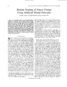
FIG. 1. Architecture of the proposed artificial neural network.
3. Artificial neural networks As described in the previous section, using the theoretical radiative model we can simulate the TOA radiances in each band from cloud and atmospheric conditions. However, because of the complexity of this model, its inversion cannot be performed in an analytical way and the utilization of numerical methods is necessary to accomplish this task. In this work neural networks techniques are proposed with this aim. The computational unit of an artificial neural network is the artificial neuron. Each of these nodes is defined by some parameter, such as the weights Wij associated with each neuron input, activation function f(u), and bias. Depending on the distribution of these neurons, several kinds of networks can be distinguished (Hristev 2000; Kröse and Smagt 1996). In this particular study, the widely used MLPs were chosen to retrieve cloud properties, where the units are located in layers and there are not connections between units in the same layer (Fig. 1). Data processing is done in hidden and output layers, with the activation function being the only possible difference between both kinds of units. In this case, the logistic function is used for both hidden and output neurons (Thim and Fiesler 1997). This function is continuous, increasingly monotone, and enclosed in a particular interval, and so a normalization of training data is necessary. Logistic function avoids both saturation when intense signals are introduced in the network and attenuation when signals are too weak. To define the architecture of the network, the optimal number of layers and hidden neurons must be determined, that is, the structure that provides the best configuration of weights (Chester 1990; Lawrence et al. 1996; Zhang et al. 1998). These parameters depend on several factors, such as the number of input and output units, the amount of available training patterns, the complexity of the problem, and the used training algo-
JANUARY 2007
CERDEÑA ET AL.
rithm. These elements must be studied in detail in order to avoid overfitting or underfitting and to increase the ability of generalization of the ANN.
a. Training algorithm During the training stage, the weights matrix is fitted gradually until the output vector is close to the desired value. The training algorithm has an important influence on the generalization ability. In this work, a supervised algorithm, called backpropagation with momentum, is used to train the network. This algorithm is described by the following learning procedure: let us assume a neural network with Ni input units, Nh hidden units, and No output units. This network has an associated weights matrix, so that the weight wij quantifies the relationship between the neurons i and j. A training pattern {xk; k ⫽ 1, 2, . . . , Ni} is introduced in the network, and it goes forward to the output layer. The results are compared with desired targets, computing the associated mean-square error. This error goes backward to the input layer, and the error gradient is determined for each neuron. Using these values, the adjustment of the weights matrix is obtained according to W共t ⫹ 1兲 ⫽ W共t兲 ⫺ · 共E兲 ⫹ ⌬关W共t ⫺ 1兲兴,
共1兲
where (E) is the matrix of error gradient, is the learning rate, and is called the momentum parameter. This last term takes into account the previous adaptations of weights in the learning process, providing stability to the learning algorithm and becoming more insensitive to possible small perturbations in the error surface.
b. Neural network configuration In this study, the Stuttgart Neural Network Simulator (SNNS) package, created by the Institute for Parallel and Distributed High Performance System of the University of Stuttgart, was used (Zell et al. 1995). This package allows users to design and train networks with different characteristics. The importance of the solar component in daytime data makes necessary the design of two independent neural networks associated with nighttime and daytime images, respectively. Concerning nighttime images, radiances are available only in thermal infrared channels. As a consequence, in this particular case, six input neurons are necessary: surface brightness temperatures (Ts3, Ts4, and Ts5) associated with the three thermal channels, and the brightness temperatures measured by
55
AVHRR in these spectral bands (T3, T4, and T5). Furthermore, networks have three output neurons, one for each cloud parameter to retrieve cloud temperature, optical depth, and effective droplet radius. The continuous ranges of these parameters are the same as those used to generate the LUTs. For the learning stage, a dataset of 30 000 patterns was generated, which was split into a training and a validation set, containing 20 000 and 10 000 patterns, respectively. Regarding daytime study, radiances are provided by the five AVHRR channels. Furthermore, other factors must be considered, such as the annual variation of the distance between the earth and the sun or the geometry of the sun–satellite–earth system through appropriate zenith and azimuth angles. In this way, the number of input parameters increases, making the neural network structure more complex. Therefore, the final network has 11 inputs and 3 outputs. In this case, a dataset of 90 000 patterns was generated, and split into a training and a validation set with 60 000 and 30 000 patterns, respectively. To determine the optimal architecture of the neural networks, some of them with different dimensions were trained using backpropagation with momentum. Each of them was trained 10 times, with the weights matrix randomly initialized. Concerning the values of learning rate and momentum, we must take into account that large or small values of these parameters add difficulty to the convergence. Initially they were chosen as 0.2 and 0.65, respectively. The means of final validation error and associated standard deviation are shown in Fig. 2a for nighttime data, and in Fig. 2b for daytime data. In both cases, it can be concluded that networks with two hidden layers have a better generalization performance. In this way, the best network obtained for nighttime study has 100 neurons in the first hidden layer and 20 in the second one, whereas for daytime study the network with the best generalization ability has 90 and 40 neurons, respectively. Once the architecture of the ANNs has been selected, the values of the characteristic parameters associated to the training algorithm must be determined to minimize the validation error. Thus, several networks were trained using different values of learning rate and momentum. The lowest errors appear for a learning rate of 0.5 and a 0.2 momentum for nighttime study, and, for the daytime case, these parameters are 0.2 and 0.25, respectively. There are two other parameters that influence the training algorithm. They are the “flat spot elimination constant” and the “error threshold.” The first, which accelerates the training procedure in very flat regions of
56
JOURNAL OF ATMOSPHERIC AND OCEANIC TECHNOLOGY
VOLUME 24
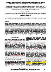
FIG. 3. Comparison of validation curves computed through three different algorithms: backpropagation with momentum, scaled conjugate gradient, and backpropagation with adaptative weights decay.
using backpropagation with momentum converges faster, and its final validation error is lower, although it is close to the results obtained with conjugate gradient procedure.
4. Genetic algorithms
FIG. 2. Comparison of the mean-square error of the validation set for networks with a different number of hidden neurons for (a) nighttime and (b) daytime cases.
the error surface, was set to zero in order to avoid training divergences. Concerning the threshold of error, it tries to accelerate the convergence. So, if the error associated to one neuronal output is smaller than this parameter, it is rounded toward zero and thereby not propagated. Thus, its value should not be large, because, although in that case the convergence of training would be faster, the generalization performance will be poor. Therefore, this parameter was also defined as zero. Finally, it must be verified that the best results are obtained using a backpropagation with momentum algorithm. Thus, this algorithm was compared with others, such as “scaled conjugate gradient algorithm” and “resilient backpropagation with adaptative weights decay algorithm.” As shown in Fig. 3, the ANN trained
The use of artificial neural networks has some important disadvantages. Thus, the performance of networks highly depends on their architecture and their characteristic parameters, or the training algorithm can get stuck in a poor local minimum of error surface. Because of these problems, the network configuration can be relatively far from the optimal one and, generally, it leads to an overestimation of the retrieved cloud parameters. The evolutionary algorithms, and genetic algorithms in particular, are useful in overcoming some of these problems. Genetic algorithms evolve a population of individuals, which represents a set of candidate solutions of a particular problem. This characteristic allows us to explore several points in the search space simultaneously, and to set the neural network’s parameters. In this way, the probability of reaching the global minimum of the error surface and determining the optimal architecture significantly increases, overcoming the disadvantages of neural networks. Consequently, the combined use of both processes reduces the necessary computation time and optimizes the neural networks’ ability of generalization (Mandischer 1993; Obradovic and Srikumar 2000; Seiffert 2001). The evolutionary artificial neural networks were ap-
JANUARY 2007
CERDEÑA ET AL.
plied using the ENZO package (Braun and Ragg 1996), developed by the Institute for Logic, Complexity and Deduction Systems of the University of Karlsruhe. This simulator uses training algorithms defined by the SNNS package, and it allows us to optimize the architecture and the weights matrix simultaneously. In this case, each network was defined using a genotypic low-level representation, where each network parameter (number and distribution of neurons, weights, connections, etc.) is specified. This algorithm works as follows. First, taking into account a reference network, an initial population is generated whose number of individuals is constant along the procedure. In this case, the used reference networks were those obtained through the studies mentioned in section 3. Once the initial set of networks has been created the training process starts using backpropagation with momentum. This training stage is stopped either when learning error is lower than a previously defined threshold value or when the maximum number of epochs has been exceeded. After the learning stage a fitness value is assigned to each individual, which evaluates its learning properties and its topology. This fitness function takes into account several factors, such as the mean training error, the number of weights and hidden units, and, to a lesser extent, the number of learning epochs needed. Using these fitness values the selection stage takes place, in which the best individuals are chosen from the population for later application of genetic operators. This package provides crossover and mutation operators, and each of them has an associated probability of application whose optimal values must be determined. In this way, prioritizing the crossover of parents, the danger of getting stuck in a local optimum increases because of the fact that individuals of a population are functionally identical. On the contrary, if mutation is the only process used, the searching procedure turns into random algorithm, making the convergence difficult. Regarding mutation, it can delete hidden neurons, insert new units, or modify the existing nodes’ characteristics. The new offspring created are trained in the same way in which the members of initial population were, and the fitness value is computed for each of them. The best networks are inserted in the population, thereby removing the worst elements. The use of genetic algorithms simplifies the neural network structure. Thus, the networks trained for nighttime study were simplified to a network with 20 units in the first hidden layer, and 5 in the second. For the daytime case, the resulting networks have approximately 50 neurons in the first hidden layer and 9 in the
57
second. Moreover, these layers of units are not completely connected to each other, because the evolutionary process gets rid of unnecessary weights.
5. Sensitivity analysis The precision of the retrieval methods is an important issue, because small changes in the characterization of low-level stratiform clouds have a large influence on global climate models (Miles et al. 2000). Thus, to evaluate the robustness of the method, the different sources of uncertainties have been analyzed. These uncertainties arise as a result of errors in satellitemeasured radiances and in general assumptions, such as fully cloudy pixels or the specification of the atmospheric properties and the lower boundary conditions, that is, surface albedo and temperature. In addition, some errors can be introduced during the inversion procedure. Those methods, based on an iterative search of the satellite-measured radiances that best fit entries in different LUTs (Nakajima and Nakajima 1995; Platnick et al. 2003), do not introduce appreciable noise in the retrieval, provided that an accurate interpolation is used and that those regions of the solution space where multiple solutions are possible, mainly for low optical thickness and small droplets, are avoided. However, in this work, the retrieval is performed by modeling the relationship between the satellite measurements and cloud parameters through ANNs. For this reason, the uncertainties caused by the ANN inversion have been studied. For the daylight case, the errors are smaller than 0.15 m in effective radius, 0.01 K in cloud-top temperature, and 0.2 in optical thickness. For the nighttime procedure, errors are smaller than 0.25 m in reff, 0.02 K in Tc, and 0.3 in . Table 1 shows the errors in the retrieved cloud parameters resulting from uncertainties in satellitemeasured brightness temperatures and surface temperatures. These results were obtained using a large number of simulations and introducing observational errors of 0.5 K in temperature, taking into account not only the in-flight noise-equivalent error but also possible solar contamination of the Internal Calibration Target (ICT) and long-term variations in calibration gains of the AVHRR (Trishchenko et al. 2002). The reported errors represent mean values over a wide range of conditions, and were divided into two groups corresponding to optically thin (optical thickness ⬍ 2) and thick ( ⬎ 8) clouds. Larger errors in retrieved effective radius (reff) and cloud temperature (Tc) correspond to thin clouds. In this situation, resulting from the relatively minor influence of cloud layer in total received radiances, small errors in measured tempera-
58
JOURNAL OF ATMOSPHERIC AND OCEANIC TECHNOLOGY
TABLE 1. Errors in retrieved cloud parameters for nighttime imagery resulting from uncertainties in satellite-measured brightness temperatures (T3, T4, and T5) and interpolated surface temperatures (Ts3, Ts4, and Ts5). The last row shows the total absolute error resulting from simultaneous uncertainties in all measurements. Errors in retrieved parameters reff (m)
Tc (K)
Uncertainties
⬍2
⬎8
⬍2
⬎8
⬍2
⬎8
T3 (0.5 K) T4 (0.5 K) T5 (0.5 K) Ts3 (0.5 K) Ts4 (0.5 K) Ts5 (0.5 K) Total
1.33 ⫺4.29 3.64 ⫺1.85 3.51 ⫺3.05 4.42
1.10 ⫺1.34 1.42 ⫺0.10 0.02 ⫺0.07 1.91
⫺3.24 ⫺1.83 3.33 2.27 1.66 ⫺2.91 3.94
⫺0.03 ⫺0.17 0.82 0.01 0.01 ⫺0.01 0.93
⫺0.19 ⫺0.27 0.53 0.32 0.13 ⫺0.02 0.63
⫺0.66 ⫺4.97 1.06 0.28 0.31 0.08 5.57
tures imply larger changes in cloud properties to counteract them. Moreover, for thin clouds, small variations in optical thickness are enough to produce large alterations in cloud radiative properties, which explain why errors in this cloud parameter are generally smaller than those for thick clouds. It also can be observed that the main source of errors is due to uncertainties in the brightness temperatures of channels 4 and 5. Furthermore, deviations in the computation of surface temperatures, interpolated from cloudless pixels, are important only for optically thin clouds. The last row of Table 1 shows the total uncertainties in retrieved cloud parameters resulting from simultaneous errors in all satellite-measured and surface temperatures. The larger errors correspond again to very low optical thickness and small particles. For optical thickness, the larger uncertainties arise primarily for very dense clouds ( ⬎ 20) because of the asymptotic behavior of emissivity in infrared channels (Fig. 4). It can also be seen that the uncertainties resulting from errors in satellite measurements and surface-estimated temperatures are significantly larger than the errors introduced by the neural network–based inversion. Table 2 summarizes the results obtained for the daylight retrieval procedure. Although degradations of the visible channel of the AVHRR have been considered for calibration of sensor signals (Rao and Chen 1999), a remaining error between 1% and 4% must be expected in cloudy scenes (Deneke et al. 2005). Thus, an observational error of 5% has been selected to perform the sensitivity study. The results are very similar to those of the nighttime case, but now the uncertainties in channel-1 reflectance also contribute to errors in the retrieved optical thickness. Moreover, the influence of the geometry (satellite and sun positions) is important during daylight, mainly affecting the retrieved reff and .
VOLUME 24
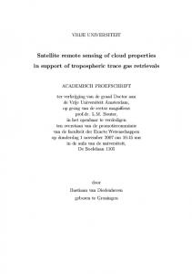
For these parameters, the errors are larger for large solar zenith angle and backward scattering. From Tables 1 and 2 it can be seen that errors in each retrieved cloud parameter depend on uncertainties in every satellite measurement. This is due to the fact that cloud parameters are highly interrelated, so, for a particular set of measured radiances, it is not possible to change only one parameter without affecting the other two. For example, channel-3 brightness temperature is most sensitive to changes in cloud droplet size, with channel-4 and -5 temperatures and channel-1 reflectance being more insensitive to variations of this parameter (Nakajima and King 1990; Perez et al. 2000). However, larger errors in retrieved effective radii correspond to uncertainties in T4 and T5. An increase in these brightness temperatures can be explained by a lower optical thickness (part of the observed radiances corresponds to surface contribution transmitted through the cloud) or a higher cloud temperature. In both cases, if T3 remains unchanged, the only possibility is that the emissivity in channel 3 is modified as a consequence of droplet size variation. A similar behavior can be expected for uncertainties in channel-1 reflectance, as is shown in Fig. 4. This figure displays the correlation between AVHRR channels 1 and 3 and channels 1 and 4 for different droplet sizes and cloud temperatures. The effect of errors in channel-1 measurements on the retrieved parameters depends on the cloud optical thickness. Thus, for a cloud with a medium optical thickness ( ⫽ 4) and an effective droplet radius of 12 m, represented by point A, an error in R1, point B, can be explained by, in addition to an increment in optical thickness, changes in droplet size (Figs. 4a and 4b) or cloud temperature (Figs. 4c and 4d). However, for a larger optical thickness ( ⫽ 8), point C, an error in R1 can be explained only by a change in optical thickness or in effective droplet radius. If the brightness temperature in channel 4 remains unchanged, the retrieved cloud temperature does not vary, as can be seen in Fig. 4d, where the point D belongs to the curve of the same cloud temperature. Thus, the link from points C to D in Fig. 4c is not possible. This behavior can be observed in the first row of Table 2. Furthermore, the sensibilities of uncertainties in the total atmospheric water vapor or cloud fraction were studied, finding smaller effects than those for brightness temperature deviations. As it is known, the water vapor is mainly located under the cloud layer, so its effect is considered in the interpolated surface temperatures. The larger errors resulting from partially covered pixels correspond to the retrieved effective radius, as occurs with optically thin clouds.
JANUARY 2007
CERDEÑA ET AL.
59
FIG. 4. Correlations between AVHRR channels 1 and 3 and channels 1 and 4 for (a), (b) different cloud droplet effective radii and (c), (d) different cloud temperatures. Following the curves from left to right the cloud optical thickness increases as i ⫽ 0.125, 0.25, 0.5, 1, 2, 4, 8, 16, 32, and 64. The cloud temperature is 284 K for (a), (b) and the particle size is 12 m for (c), (d). Calculations are for a solar zenith angle of 40°, satellite zenith angle of 10°, and azimuth of 50°. The meaning of points A, B, C, and D is explained in the text.
The retrieval uncertainties have been compared with those provided in other retrieval procedures. Sensitivity studies of cloud retrieval procedures are usually applied to realistic clouds (Nakajima and Nakajima 1995), that is, optically thick layers and medium effective droplet radius. In these conditions (5 ⬍ ⬍ 30 and reff ⬃ 10 m), and for errors of 10% in satellite measurements and surface temperatures estimation, the global absolute uncertainties of the proposed retrieval method are 0.8 m (8%) for reff, 0.9 K (0.3%) for Tc, and 2.1 (18%) for in the nighttime case. For the daylight retrieval the uncertainties are 0.7 m (7%), 0.9 K (0.3%), and 1.0 (8%), respectively. These errors in optical thickness are
lower than those shown in Tables 1 and 2, because the larger errors appear for very large optical thickness, resulting from the asymptotic behavior of reflectance and brightness temperatures. Platnick and Valero (1995) estimated that a 10% uncertainty in the channel-3 reflectance roughly corresponds to an equivalent 10% uncertainty in the retrieved size. Han et al. (1994) similarly estimated retrieval errors for their study to be 1–2 m. Nakajima and Nakajima (1995) presented retrieval errors lower than 10% for optical thickness and droplet size. Similar uncertainties are estimated by Platnick et al. (2000) for droplet size retrieval using spectral bands centered at 1.62 and 2.13 m. Platnick et
60
JOURNAL OF ATMOSPHERIC AND OCEANIC TECHNOLOGY
TABLE 3. Comparison of in situ–measured radii and those obtained using ANN and GA for nighttime data.
TABLE 2. Errors in retrieved cloud parameters for daytime imagery resulting from uncertainties in satellite-measured channel-1 reflectance (R1), brightness temperatures (T3, T4, and T5), and interpolated surface temperatures (Ts3, Ts4, and Ts5). The last row shows the total absolute error resulting from simultaneous uncertainties in all measurements. Errors in retrieved parameters reff (m)
Tc (K)
Uncertainties
⬍2
⬎8
⬍2
⬎8
⬍2
⬎8
R1 (5%) T3 (0.5 K) T4 (0.5 K) T5 (0.5 K) Ts3 (0.5 K) Ts4 (0.5 K) Ts5 (0.5 K) Total
⫺1.05 ⫺1.00 ⫺3.77 2.53 0.14 1.94 ⫺2.86 3.93
⫺0.53 ⫺0.57 ⫺1.57 1.22 ⫺0.29 ⫺0.28 ⫺0.32 1.82
1.48 0.47 ⫺3.16 3.36 ⫺0.58 2.21 ⫺2.82 4.20
0.04 0.01 ⫺0.47 0.90 0.01 0.01 ⫺0.01 0.96
0.46 0.08 ⫺0.14 0.33 0.05 0.24 0.01 0.41
1.99 ⫺0.29 ⫺2.66 1.39 ⫺0.24 ⫺0.22 ⫺0.26 2.83
al. (2001) obtained uncertainties of about 8% in droplet size and 20% in optical thickness for retrievals based on 0.67- and 3.7-m reflectance and errors of 10%. These uncertainties are expected to be reduced with the newgeneration sensors, like the National Polar-orbiting Operational Environmental Satellite System (NPOESS) Visible–Infrared Imager–Radiometer Suite (VIIRS) (Higgins and George 2000; Ou et al. 2002). While the threshold requirements for the retrieved cloud parameters precision (5% or 2 m for reff, 1.5 K for Tc, and 5% or 0.025 for ) are met by most of retrieval procedures, the threshold objectives are quite restrictive (2% for reff, 0.5 K for Tc, and 5% or 0.025 for ). For this reason, the methods proposed for this sensor use auxiliary data such as temperature, pressure, and moisture profiles to improve retrieval results.
6. Results To validate the proposed retrieval, the results were compared with near-coincident ground-based measurements at the north of Tenerife Island. The sampling site is located on a ridge at an elevation of 922 m and is frequently immersed in the cloud layer, principally during the summer season. Taking into account that there are not significant pollution sources upwind of the site, and its geographic location, the measurements are representative of the marine stratocumulus layer characteristics (Borys et al. 1998). In-cloud microphysical properties were obtained from a Particle Measuring System (PMS) Forward Scattering Spectrometer Probe (FSSP; 100HV) optical sensor. The sampling point is estimated to represent the midpoint of the cloud as derived from balloon soundings.
VOLUME 24
Date 11 29 30 5 5 8 19 20 25 26
Jun 1995 Jun 1995 Jun 1995 Jul 1995 Jul 1996 Jul 1996 Jul 1996 Jul 1996 Jul 1996 Jul 1996
In situ measurements (m)
ANN (m)
GA (m)
5.4 5.7 5.1 4.8 9.1 7.9 5.9 5.8 6.3 7.7
5.7 6.5 6.9 5.5 8.6 8.7 6.8 5.6 6.8 7.6
5.3 6.2 6.7 5.2 8.7 8.5 6.8 5.1 6.8 7.6
Table 3 shows the results computed from different images for the most sensible and difficult to obtain parameter, the droplet size. This table compares effective droplet radii retrieved using the genetic algorithm (GA) in the learning stage and applying the neural network that was determined in section 3b. These algorithms give reasonable results and they reproduce the tendency of effective sizes. Regarding the method of designing and training the neural networks, the use of genetic algorithms produces results nearer in situ data. The average difference between retrieved and in situ measurements is 0.66 m for ANN results and 0.58 m for evolutionary neural networks. Moreover, the significant decrease in computation time turns GA into a powerful numerical method. When these values are analyzed, the cloud properties’ variation within the region that has been chosen to average the results must be considered. These horizontal inhomogeneities in cloudy layers are obvious in Figs. 5b, 5c, and 5d, where effective radius, optical thickness, and cloud temperature are shown. In this figure, black areas correspond to land—the Canary Islands and West African coast—while detected cloudless pixels are colored gray in Figs. 5b and 5d. It can be observed that the retrieved cloud-top temperature is quite homogeneous as can be expected for a stratiform layer, while the retrieved optical thickness shows a textured appearance, typical in stratocumulus clouds. The effective radius provides a smooth-textured image, where larger sizes generally correspond to optically thick regions. Several authors (Nakajima and Nakajima 1995; Szczodrack et al. 2001) have shown that optically thin water clouds (with optical thickness lower than 15) over the ocean tend to have a positive correlation between effective droplet radius and optical thickness. In Table 4, retrieved effective radii are shown as function of the method used to train the networks for
JANUARY 2007
CERDEÑA ET AL.
61
FIG. 5. Cloud parameters retrieved for an image acquired at 1400 UTC 5 Jul 1996: (a) AVHRR channel-4 image, (b) effective radius, (c) optical thickness, and (d) cloud temperature. Land is colored black and the detected cloudless pixels are colored gray.
the daylight case. In this case, the optimization of neural networks performance is more remarkable. The average errors of retrieved effective droplet sizes are 1.3 and 0.54 m when applying artificial neural networks
and evolutionary algorithms respectively. These results corroborate that genetic algorithms optimize the neural networks behavior. The resultant neural networks, after the genetic al-
62
JOURNAL OF ATMOSPHERIC AND OCEANIC TECHNOLOGY TABLE 4. Comparison of in situ–measured radii and those obtained using ANN and GA for daytime data.
Date 5 7 8 18 20 25 26
Jul Jul Jul Jul Jul Jul Jul
1996 1996 1996 1996 1996 1996 1996
In situ measurements (m)
ANN (m)
GA (m)
9.1 7.6 7.9 5.5 5.8 8.3 7.7
10.8 10.1 7.9 6.5 5.9 7.1 5.0
9.5 9.2 7.8 6.0 5.5 7.6 7.9
gorithms optimization, provide a computationally efficient method for obtaining cloud parameters. For the nighttime case this procedure needs around 2950 floating point operations (FLOPs) per cloudy pixel, while for the daylight case it needs around 10 870 FLOPs. This performance is approximately one order of magnitude higher than other widely used techniques, such as the dual-channel correlation approach applied to MODIS data (King et al. 1997).
7. Concluding remarks The development of an inversion method of a radiative transfer model to determine cloud properties requires the use of numerical techniques. Among several existing tools artificial neural networks were chosen, because of their ability of generalization and their low computation time. Although the learning process can be quite time consuming, the use of a trained network takes up little time, which is an important characteristic when a temporal study is carried out using large datasets. Artificial neural networks are defined by numerous parameters, whose values must be determined to optimize results. This optimization was made using genetic algorithms, which increase the probability of finding the optimal network. This network is characterized by a simple structure containing fewer weights and neurons. In this work, the proposed method has been applied to AVHRR imagery; however, it can be easily extended to new-generation sensors, such as, MODIS, the Spinning Enhanced Visible and Infrared Imager (SEVIRI), etc. These radiometers have spectral bands that are very similar to those included in the AVHRR nighttime and daylight retrieval methods. Moreover, these new sensors provide additional channels that can be used to infer other cloud or atmospheric properties. Both the comparison between cloud parameters obtained through the proposed method and ground-based measurements allow us to show the good performance of neural networks. Furthermore, evolutionary algo-
VOLUME 24
rithms improve the results, showing their applicability to the optimization process of the nets for both nighttime and daytime studies. Although this work shows reasonable results, further studies are required to fully validate the method. Acknowledgments. The authors wish to express their gratitude to Ministerio de Ciencia y Tecnología of Spain (Project REN2003-08013) and to Fondo Europeo de Desarrollo Regional (FEDER) for financial support. The authors also wish to acknowledge the reviewers, who made several helpful suggestions after reviewing an earlier version of this paper. REFERENCES Anderson, G. P., S. A. Clough, F. X. Kneizys, J. H. Chetwynd, and E. P. Shettle, 1986: AFGL atmospheric constituent profiles (0–120 km). Hanscom Air Force Base, AFGL Tech. Rep. AFGL-TR-86-0100, 46 pp. Baum, B. A., R. F. Arduini, B. A. Wielicki, P. Minnis, and S. Tsay, 1994: Multilevel cloud retrieval using multispectral HIRS and AVHRR data: Nighttime oceanic analysis. J. Geophys. Res., 99, 5499–5514. ——, R. Frey, G. G. Mace, M. K. Harkey, and P. Yang, 2003: Nighttime multilayered cloud detection using MODIS and ARM data. J. Appl. Meteor., 42, 905–919. Borys, R. D., D. H. Lowenthal, M. A. Wetzel, F. Herrera, A. Gonzalez, and J. Harris, 1998: Chemical and microphysical properties of marine stratus clouds in the North Atlantic. J. Geophys. Res., 103, 22 073–22 085. Braun, H., and T. Ragg, 1996: ENZO: Evolution of neural networks. User manual and implementation guide, University of Karlsruhe, 62 pp. Brenguier, J. L., H. Pawlowska, L. Schüller, R. Preusker, J. Fischer, and Y. Fouquart, 2000: Radiative properties of boundary layer cloud: Droplet effective radius versus number concentration. J. Atmos. Sci., 57, 803–821. Chester, D. L., 1990: Why two hidden layers are better than one. Proc. Int. J. Conf. Neural Network, 1, 265–268. Coakley, J. A., and F. P. Bretherton, 1982: Cloud cover from high resolution scanner data: Detecting and allowing for partially filled fields of views. J. Geophys. Res., 87, 4917–4932. Cox, C., and W. Munk, 1954: Measurement of the roughness of the sea surface from photographs of the sun’s glitter. J. Opt. Soc. Amer., 44, 838–850. Deneke, H., A. Feijt, A. van Lammeren, and C. Simmer, 2005: Validation of a physical retrieval scheme of solar surface irradiances from narrow-band satellite radiances. J. Appl. Meteor., 44, 1453–1466. Gonzalez, A., J. C. Perez, F. Herrera, F. Rosa, M. A. Wetzel, R. D. Borys, and D. H. Lowenthal, 2002: Stratocumulus properties retrieval method from NOAA-AVHRR data based on the discretization of cloud parameters. Int. J. Remote Sens., 23, 627–645. Han, Q., W. B. Rossow, and A. A. Lacis, 1994: Near-global survey of effective droplet radii in liquid water clouds using ISCCP data. J. Climate, 7, 465–497. Han, W., K. Stamnes, and D. Lubin, 1999: Remote sensing of surfaces and clouds properties in the arctic from AVHRR measurements. J. Appl. Meteor., 38, 989–1012.
JANUARY 2007
CERDEÑA ET AL.
Higgins, G. J., and A. George, cited 2000: Cloud top parameters. Visible/Infrared Image/Radiometer Suite (VIIRS). Raytheon Systems Company, Algorithm Theoretical Basis Document SBRS Doc. Y2399. [Available online at http://npoesslib.ipo. noaa.gov.] Hristev, R. M., 2000: Matrix techniques in artificial neural networks. M.S. thesis, Department of Mathematics and Statistics, University of Canterbury, 174 pp. Kawamoto, K., T. Nakajima, and T. Y. Nakajima, 2001: A global determination of cloud microphysics with AVHRR remote sensing. J. Climate, 14, 2054–2068. King, M. D., S.-C. Tsay, S. E. Platnick, M. Wang, and K.-N. Liou, 1997: Cloud retrieval algorithms for MODIS: Optical thickness, effective particle radius, and thermodynamic phase (MOD06). NASA Goddard Space Flight Center Rep. ATBD-MOD-05, 79 pp. Kokhanovsky, A. A., V. V. Rozanov, P. E. Zege, H. Bovensmann, and J. P. Burrows, 2003: A semi-analytical cloud retrieval algorithm using backscattered radiation in 0.4–2.4 m spectral region. J. Geophys. Res., 108, 4008, doi:10.1029/ 2001JD001543. Kröse, B., and P. V. D. Smagt, 1996: An Introduction to Neural Networks. University of Amsterdam, 135 pp. Lawrence, S., C. L. Giles, and A. C. Tsoi, 1996: What size neural network gives optimal generalization? Convergence properties of backpropagation. Institute for Advanced Computer Studies, University of Maryland Rep. UMIACS-TR-96-22 and CS-TR-3617, 35 pp. Mandischer, M., 1993: Representation and evolution of neural networks. Artificial Neural Nets and Genetic Algorithms Proceedings of the International Conference at Innsbruck, Austria, C. R. R. F. Albrecht, and N. Steele, Eds., Springer, 643–649. Mayer, T., and A. Killing, 2005: Technical note: The libradtran software package for radiative transfer calculations: Description and examples of use. Atmos. Chem. Phys., 5, 1855–1877. Miles, N. L., J. Verlinde, and E. E. Clothiaux, 2000: Cloud droplet size distribution in low-level stratiform clouds. J. Atmos. Sci., 57, 295–311. Minnis, P., K. N. Liou, and Y. Takano, 1993: Inference of cirrus cloud properties using satellite-observed visible and infrared radiances. Part I: Parameterization of radiance fields. J. Atmos. Sci., 50, 1279–1304. Nakajima, T., and M. D. King, 1990: Determination of the optical thickness and effective particle radius of clouds from reflected solar radiation measurements. Part I: Theory. J. Atmos. Sci., 47, 1878–1893. ——, ——, J. D. Spinhirne, and L. F. Radke, 1991: Determination of the optical thickness and effective particle radius of clouds from reflected solar radiation measurements. Part II: Marine stratocumulus observations. J. Atmos. Sci., 48, 728–750. Nakajima, T. Y., and T. Nakajima, 1995: Wide-area determination of cloud microphysical properties from NOAA AVHRR measurements for FIRE and ASTEX regions. J. Atmos. Sci., 52, 4043–4059. Obradovic, Z., and R. Srikumar, 2000: Constructive neural networks design using genetic optimization. Ser. Math. Inf., 15, 133–146. Ou, S. C., K. N. Liou, W. M. Gooch, and Y. Takano, 1993: Remote sensing of cirrus cloud parameters using Advanced Very-High-Resolution Radiometer 3.7 and 10.9 m channels. Appl. Opt., 32, 2171–2180.
63
——, ——, Y. Takano, G. J. Higgins, A. George, and R. Slonaker, cited 2002: Cloud effective particle size and cloud optical thickness. Visible/Infrared Image/Radiometer Suite (VIIRS). Raytheon Systems Company Advanced Theoretical Basis Document SBRS Doc. Y2395. [Available online at http:// npoesslib.ipo.noaa.gov.] Perez, J. C., F. Herrera, F. Rosa, A. Gonzalez, M. A. Wetzel, R. D. Borys, and D. H. Lowenthal, 2000: Retrieval of marine stratus cloud droplet size from NOAA-AVHRR nighttime imagery. Remote Sens. Environ., 73, 31–45. ——, P. H. Austin, and A. González, 2002: Retrieval of boundary layer cloud properties using infrared satellite data during the DYCOMS-II field experiment. Proc. 15th Symp. of Boundary Layer and Turbulence, Wageningen, Netherlands, Amer. Meteor. Soc., CD-ROM, 5.3. Platnick, S., and S. Twomey, 1994: Determining the susceptibility of cloud albedo to changes in droplet concentration with Advanced Very High Resolution Radiometer. J. Appl. Meteor., 33, 334–347. ——, and F. P. J. Valero, 1995: A validation of satellite cloud retrieval during ASTEX. J. Atmos. Sci., 52, 2985–3001. ——, and Coauthors, 2000: The role of background cloud microphysics in the radiative formation of ship tracks. J. Atmos. Sci., 57, 2607–2624. ——, J. Y. Li, M. D. King, H. Gerber, and P. V. Hobbs, 2001: A solar reflectance method for retrieving cloud optical thickness and droplet size over snow and ice surfaces. J. Geophys. Res., 106, 15 185–15 199. ——, M. D. King, S. A. Ackerman, W. P. Menzel, B. A. Baum, J. C. Riedi, and R. A. Frey, 2003: The MODIS cloud products: Algorithms and examples from Terra. IEEE Trans. Geosci. Remote Sens., 41, 459–473. Ramanathan, V., 1987: The role of earth radiation budget studies in climate and general circulation research. J. Geophys. Res., 92, 4075–4095. Rao, C. R. N., and J. Chen, 1999: Revised post-launch calibration of the visible and near-infrared channels of the Advanced Very High Resolution Radiometer on the NOAA-14 spacecraft. Int. J. Remote Sens., 20, 3485–3491. Seiffert, U., 2001: Multiple layer perceptron training using genetic algorithms. Proc. European Symp. on Artificial Neural Networks ESANN, Bruges, Belgium, ESANN, 159–164. Stamnes, K., S. Tsay, W. Wiscombe, and K. Jayaweera, 1988: Numerically stable algorithm for discrete-ordinate-method radiative transfer in multiple scattering and emitting layered media. Appl. Opt., 27, 2502–2509. Szczodrack, M., P. H. Austin, and P. B. Ktummel, 2001: Variability of optical depth and effective radius in marine stratocumulus clouds. J. Atmos. Sci., 58, 2912–2926. Thim, G., and E. Fiesler, 1997: Optimal setting of weights, learning rate and gain. IDIAP Research Rep. 97-04, 15 pp. Trishchenko, A. P., G. Fedosejevs, Z. Li, and J. Cihlar, 2002: Trends and uncertainties in thermal calibration of AVHRR radiometers onboard NOAA-9 to NOAA-16. J. Geophys. Res., 107, 4778, doi:10.1029/2002JD002353. Zell, A., and Coauthors, 1995: SNNS: Stuttgart Neural Network Simulator. User’s manual, version 4.1, University of Stuttgart Rep. 6/95, 350 pp. [Available online at http://wwwra.informatik.uni-tuebingen.de/SNNS/.] Zhang, G., B. E. Fiesler, and M.-Y. Hu, 1998: Forecasting with artificial neural networks: The state of the art. Int. J. Forecasting, 14, 35–62.