indicate that the artificial neural network (ANN) estimates conifer mortality more accurately than the other approaches. Further, an analysis of its architecture ...
IEEE TRANSACTIONS ON GEOSCIENCE AND REMOTE SENSING, VOL. 34, NO. 2, MARCH 1996
398
emote Sensing of Forest Change sing Artificial Neural Networks Sucharita Gopal and Curtis Woodcock, Associate Member, IEEE
Abstract-A prolonged drought in the Lake Tahoe Basin in California has resulted in extensive conifer mortality. This phenomenon can be analyzed using (multitemporal) remote sensing data. Prior research in the same region used more tradition& methods of change detection [SI, [30]. This paper introduces a third approach to change detection in remote sensing based on artificial neural networks. The neural network architecture used is a Multilayer Feedforward Network. The results of the study indicate that the artificialneural network (ANN) estimates conifer mortality more accurately than the other approaches.Further, an analysis of its architecture reveals that it uses identifiable scene characteristics-the same as those used by a GrammSchmidt transformation.ANN models offer a viable alternative for change detection in remote sensing.
I. INTRODUCTION EURAL networks hold the potential for improving a variety of tasks in remote sensing and image processing. They represent a fundamentally different approach to problems like pattern recognition, as they do not rely on statistical relationships. Instead, neural networks adaptively estimate continuous functions from data without specifying mathematically how outputs depend on inputs (Le., adaptive model-free function estimation using a nonalgorithmic strategy). To date, most of the efforts to use neural networks in remote sensing have involved image classification with considerable success (e.g., [2], [12], [14], [18], [22]). Neural network classifiers outperform conventional classifiers mainly due to their lack of assumptions about normality in datasets, considerable ease in using multidomain datasets, and perhaps, in capturing some of the inherent nonlinearity in such data. The purpose of this paper is to test the utility of neural networks in change detection. As far as we know, this is the first paper to use neural networks for change detection in remote sensing. In particular, neural networks are used to estimate the degree of conifer mortality in the Lake Tahoe Basin. This area has been studied in the past [8], [30], and this project uses their datasets. Change detection studies in remote sensing involve the use of multitemporal datasets, Le., sequential images taken of the same area. Techniques to analyze the location, nature, and magnitude of changes serve two distinct purposes [37]: comparative analysis of independently produced classifications, and simultaneous analysis of multitemporal data. Singh E371 provides an excellent review and comparison of various Manuscript received December 16, 1994; revised July 20, 1995. This work was supported by the National Science Foundahon under Grant SBR-9300633 The authors are with the Department of Geography, Boston University, Boston, MA 02215 USA. Publisher Item Identifier S 0196-2892(96)01005-4.
change detection methods such as image differencing, principal component analysis, and multitemporal regression. Since that time, much additional literature has been published on the logic of change detection. In the area of timber inventory and forest management, changes in forest cover caused due to defoliation by insects [31], [32], [39], [41] and landuse andor other human-induced factors (e.g., pollution stress) [7], [9], [38] are significant. The perspective on change detection in this paper is a bit different from the normal in remote sensing, which is to detect changes in land use or land cover. In these studies the nature of the change is categorical, or between different landcover classes 1371. In this study, the intent is to measure the magnitude of change [25], [26], which in this case corresponds to the number of trees in a forest that have died. E. BACKGROUND: THE MAPPINGPROJECT AND PRIOR &PROACHES TO DETECTION OF CONIFER MORTALITY
For the past several years, Boston University Center for Remote Sensing and the U.S. Forest Service (USFS) Region 5 Remote Sensing Group have been involved in developing a set of new methods for mapping and inventorying forest vegetation using remote sensing and geographical information systems (GIS). An important innovation in this mapping project has been the use of an image segment procedure [42] to define the map units early, in the mapping process, enabling subsequent analysis to be conducted on stands rather than a per-pixel basis. The image segmentation algorithm uses raw TM bands and a texture channel and produces regions that are the polygons used in the final map. The other primary innovation is the use of a forest canopy reflectance model to map forest stand structure. An overview of the mapping ’ procedure and its results are given in Woodcock et al. [43]. During the period of this project, the region experienced prolonged drought that has resulted in considerable mortality of conifer trees. Two prior approaches for detecting conifer mortality in the Lake Tahoe Basin have been tested. Macomber and Woodcock [30] used a method that measures the decrease in crown cover between the two dates of the images. Estimates of crown cover are obtained from the Li-Strahler model [29] for each conifer stand for two dates of imagery. Three levels of change in crown cover were combined with three crown cover classes to stratify the forest areas. Field samples were collected for each stratum and total conifer mortality was estimated at 15% of the total timber volume between 1988 and 1992. The patterns in the means for the strata followed the anticipated patterns with respect to mortality, indicating the viability of
0196-2892/96$05.00 0 1996 IEEE
GOPAL AND WOODCOCK: REMOTE SENSING OF FOREST CHANGE USING ARTIFICIAL NEURAL NETWORKS
the approach. However, at the level of individual stands, the relationship between field measurements and estimated mortality were less reliable (R2 S 0.4). Collins and Woodcock [SI proposed a new change detection technique based on the Gramm-Schmidt orthogonalization process by which an n-band image may be decomposed into n-orthogonal indices, each with the potential of measuring scene characteristics. The analysis of change in Lake Tahoe used three stable components corresponding to multidate brightness, greenness, and wetness, and one change component. Regressions between these components and field measurements indicated improved ability to detect mortality compared with the methods of [30]. Depending on which data were used to train and test the regression model, adjusted R2 values ranged from approximately 0.5-0.7. 111. METHODSAND RESULTS This paper pursues a third approach to change detection based on artificial neural networks. Artificial neural networks (ANN’S) are large networks of extremely simple computational units, massively interconnected and running in parallel. Formally, an ANN may be viewed as a dynamic system with the topology of a directed graph which can execute information processing by means of its state response to continuous or episodic input [17]. The nodes of the graph are called processing elements (PE’s), and the directed links (unidirectional signal channels) are termed connections. The PE’s communicate with one another by signals that are numerical rather than symbolic. ANN’S are designed to perform a task by specifying the architecture: the number of processing elements, the network topology (i.e., the interconnections of the PE’s), and the weight or strength of each connection via learning rules. ANN’S have proven well suited to problems of pattern recognition and classification, nonlinear feature detection, prediction and function approximation [4], [ 161-[ 191, [23], [24]. The essence of learning in ANN’S is to find a suitable set of parameters that approximate an unknown input-output relation. This problem in the present context is solved using a supervised learning algorithm, which requires a training set (i.e., a set of input-output examples). Learning the training set may be posed as a search in the network parameter space by introducing an additive error function of statistically independent examples which measures the quality of the network’s approximation to the input-output relation on the restricted domain covered by the training set. The minimization of this error over the network‘s parameter space is called the training process. The ultimate goal, however, is to minimize the error for all possible examples related through the input-output relation, namely, to generalize outside of the training set [28]. Hornik, Hinton, and White [20] and Cybenko [ 111 have shown that these networks can approximate any continuous input-output relation of interest to any degree of
accuracy, provided sufficient hidden units are available. The architecture of the two-layer feedforward network considered in the present research is fixed and determined by the number of units per array and by their connectivity. The network receives a vector input signal x and emits an
399
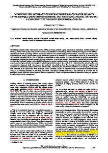
output signal x . The system has no feedback connections (see Fig. 1). The inputs units i(i = 1,.. . , I) send signals x z toward intermediate (hidden) units over connections that either attenuate or amplify signals by a factor wZ3.Each hidden unit j ( j = 1,. . . , J ) sees signals X , W , ~ (i = 1, . . . ,I) and process them in some characteristic way. In the present research, a simple function is used: the hidden unit sums what it receives and produces an activation y3 that is sent to the output units k ( k = 1,. . . , K ) . The input to the hidden unit determines the state y3 of the element through the transfer function f . A logistic function is used that scales the activation sigmoidally between 0 and 1. The bias unit (shown in Fig. 1) outputs a fixed unit value and can be viewed as constant terms in the equation defining the learning process carried out by the network. The network was trained using the backpropagation procedure that iteratively adjusts the coupling strengths in the network to minimize the error between the desired pattern and the predicted pattern. Since convergence tends to be extremely slow, the momentum variant is added to the weight update equation to achieve a faster rate of convergence [21]. At each step n, weight parameter w ( n ) of the network is updated according to the following equation:
where q and y are the learning and momentum rates, and e(x I x ) is the error signal between target vector x and output vector 2. Hence d e / d w denotes the partial derivative of the error with respect to ~ ( n )For . complete derivation of this equation see standard references on backpropagation networks [21], [36], [40]. The statistical approach to learning in such networks is described in Gopal and Fischer [15]. Data representation is a critical component in ANN modeling since it has a strong effect on what can be learned and how long it takes to learn. In the present research context, input information consists of TM data and output consists of the change in basal area between 1988 and 1991. There are two methods of representing the inppt vector: a 10-input vector of 10 TM Bands (5 for 1988 and 5 for 1991) or a 5-input vector of the differences in the five TM Bands between 1988 and 1991. Either absolute or relative change could be represented in the output vector. A decision also had to be made whether to use individual pixel information or stand (map units) information. TM data (input) were available for each pixel while change in basal area (output) was available only for stands. From the viewpoint of training the neural network, pixel-level information provides more data for training while stand-level information may provide too few training examples. But to use pixel-level input data, the stand-level output representation has to be disaggregated to the pixel level. Data on change in basal area (between 1988 and 1991) were collected during two field seasons from 26 and 61 stands, respectively. We used the set of 61 stands to train the network and 26 stands to test or estimate the generalization capability of the network. Several multilayer feedforward networks were constructed and simulations were systematically made with different input
IEEE TRANSACTIONS ON GEOSCIENCE AND REMOTE SENSING,VOL. 34, NO. 2, MARCH 1996
400
Net work Units including biases)
Network Architecture
Output Units
Network
ers
1 Output Unit
Bias Unit Hiddens Units
Input Units
Hidden Layer
k=l , ..., 15
Input Units
Fig. 1. Neural network architecture used in change detection (10:15:1).
and output representations in order to find an acceptable architecture in terms of convergence during learning and generalization. In all these simulations, input and outputs were normalized in the [O, 11 range. This normalization removes any need to transform the original digital variable like radiance. Also, additive effects associated with sensor differences between dates becomes irrelevant. We found that the best network performance was obtained using stand-level information with the 10-input vector and the output vector of the total change in basal area between the two dates of observation. There may be many reasons why this data representation produced the best performance results. Using pixel-level information, each pixel in the stand is assumed to have the mean mortality level for the stand. This assumption does not match the physical reality. The mortality withm stands is concentrated in patches with some areas exhibiting little more mortality. This mismatch at the pixel level adds noise io the neural network and undermines convergence on a solution. The result of this many-to-one mapping is that the neural network may be unable to find an appropriate mapping between the inputs and outputs. Thus, the stand-level
distribution between -0.1 and 0.1. During each time step a set of 5 input signals (i.e., epoch size of 5 ) is presented in random order (stochastic approximation). At the end of each epoch, the network parmeters are updated using (1). Simulations were made with different values of learning rate, q, and momentum rate, 7 , in (1). A final choice on their values was made that reduced oscillations during learning. These values are 0.3 and 0.6, respectively. Since the backpropagation procedure is sensitive to different starting points, five simulations with
representation proved more successful despite the dramatic
pairs are presented to the network. After aaining, the net-
reduction in the amount of available data. The other important representation question concerns the use o f the raw TM data for both dates (10-band input) versus use of only the differences between dates (5-band input). The IO-band input representation proved more useful as the 5-band input never converged to a reasonable solution. One possible reason is the loss of data concerning overall brightness associated with the use of differences. Fig. 1 shows the architecture of the network. There are 10 inputs, 15 hidden units, and one output. The initial weights in the network were drawn at random from an uniform
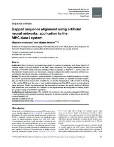
work’s generalization performance was estimated on a test dataset that was not part of the training data set. The prediction of the 10:15:1 neural network model is shown in the scatterplot in Fig. 2. The actual basal area change is plotted against the predicted basal area change. There are 26 points in the test set. There is a reasonable fit between the two as most of the points are near the diagonal: The value of adjusted R2 using the neural network prediction on the test data set was 0.839 compared to the corresponding values obtained using Gramm-Schmidt approach of between 0.48 and 0.70. Another measure of goodness of fit is the root-mean-
different random initializations were conducted. The number of hidden units was varied between 5 io 50. Best performance was produced with hidden units 15-20. Hence the minimal architecture with 15 hidden units is selected to discuss the results. Five simulations of the 10:15:1 network with different initial conditions were made. The results of the best simulation (with minimum variance) are presented in the next section, but it is interesting to note that all five simulations produced similar results. This similarity is encouraging and one indication of the stability of the input-output relationship. There are two phases in neural network modeling-training and testing. During training, input and desired output pairs
GOPAL AND WOODCOCK REMOTE SENSING OF FOREST CHANGE USING ARTIFICIAL NEURAL NETWORKS
0
50
100
401
150
Actual Basal Area Change Fig. 2. Network approximation using backpropagation (10:15:1) plot of observed versus predicted basal areas of test stands.
square error (RMSE). RMSE using Gramm-Schmidt approach varied between 9.91 to 7.86. RMSE using neural network is 6.80. These results indicate that the ANN model produces better prediction results compared to the benchmark approach.
IV. DISCUSSION One key question concerns the reason the neural network produces better estimates of conifer mortality than the Gramm-Schmidt technique. This concern is common when using neural networks, as they are often treated as “black boxes”-meaning that the nature of the signal used from the input variables and its relationship to the output are usually unknown. For applications where a one-time relationship is all that is required, this black-box approach may be sufficient. However, the more common case in pattern recognition is the desire to detect patterns usable many times, or to learn about the underlying relationships between variables. From a remote sensing perspective, neural networks will prove most useful if their internal behavior can be understood. Also, the kinds of uses for neural networks expand if their internal structure is understood. There appear to be two primary possibilities why neural networks worked better than the Gramm-Schmidt technique. First, the relationship between conifer mortality and the spectral data may be nonlinear. Given the lack of constraints in this regard within neural networks, they would have an obvious advantage in this situation. The other possibility is that the neural networks are using different patterns or a different “signal” in the spectral data to find mortality. To evaluate this situation, we explored the use of principal components analysis [ 131. Recently, several researchers [ 101, [27], [33]-[351 have explored how neural networks filter for principal components. In the present study, a covariance matrix of the hidden unit activation (weights) of the trained network was formed and the principal components were extracted. Analysis of the
eigenvalues and eigenvectors in this matrix is useful for two purposes. First the eigen values provide an indication of the relative importance of the various principal components. The first principal component explains nearly 94% of the variance in the data. The second and third explain an additional 4%. These percentages can be interpreted as the percent of the variances in the output vector (mortality) contained in the various components defined. This formulation for principal components analysis (PCA) is different from conventional applications because the information extracted relates to the dependent variable (mortality in this case). This difference in formulation is possible due to the filtering of information from the input variables related to the output variable by the weights in the neural network. All the other principal components are insignificant and are discarded from further analysis. The eigenvectors for the first three principal components and shown in Table I. The eigenvectors are direct analogs of the components created by the Gramm-Schmidt technique used by Collins and Woodcock [SI and facilitate comparison of the two methods. The first principal component is very similar to the “change” component defined using the Gramn-Schmidt procedure. (Table I1 from [8]). The pattern in the signs for the coefficients matches exactly and the magnitudes of the coefficients are also similar. This result indicates that the primary signal used by both methods is the same. Also, the second eigenvector looks in general like a multidate brightness image, much like the one defined in the Gramm-Schmidt analysis. That this factor might be related to change is interesting, and a result of the conditions in the Lake Tahoe Basin. As described by [8] and [30], there are patterns in the areas where conifer mortality is concentrated. One such pattern is that areas of the densest stocking of trees have the highest mortality. Since brightness is inversely related with forest density, there is a correlation between mortality and scene brightness. Similarly, the third eigenvector has the form of a multidate greenness index, which is also correlated with stand density and hence mortality.
IEEE TRANSACTIONS ON GEOSCIENCE AND REMOTE SENSING, VOL. 34, NO. 2, MARCH 1996
402
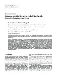
TABLE II GRAMM-SCHMIDT TRLNSFORMATION VECTORS
TM Band TM 2 1988 TM 3 1988 TM 4 1988 TM 5 1988 TM 7 1988 TM 2 1991 TM 3 1991 TM 4 1991 TM 5 1991 TM 7 1991
Principal Components 1 2 3 -0.320 0.236 0.146 -0.313 0.423 0.273 0.295 0.619 -0.611 -0.320 0.285 0.206 -0.323 0.123 0.251 0.320 0.114 0.223 0.322 0.124 0.276 -0.312 0.317 -0.314 0.319 0.269 0.281 0.317 0.292 0.350
Given that it appears that the same spectral signal is being used by both the Gramm-Schmidt technique and the neural network, it seems likely that there are nonlinearities in the relationship between the spectral inputs and the observed mortality pattems which account for the improved results using ANN'S. At this point it is possible to consider some of the strengths and weaknesses of the two methods, particularly as they apply to future use. Obviously the fact that neural networks produced better results is important. However, there are other considerations that influence decisions regarding which method to use. One such consideration is the amount of field data required to train the neural network. The GrammSchmidt technique can be calibrated by enough field sites to estimate regression coefficients-or approximately 30 sites. Neural networks need many more field sites for training the network. In this study less than one hundred sites (5334 pixels) were used, but that would appear to represent a bare minimum. A serious problem in model estimation is the problem of overfitting which is particularly serious for noisy limited real world data. Several strategies exist for handling such problems [ 11. We will address this problem in future research. Each field site represents a full day's work for two people, so this difference is not trivial. Another consideration is the nature and quantity of processing required for the two different approaches. The processing for the Gramm-Schmidt technique is direct and relatively easy. On the other hand, error-based neural networks such as the backpropagation that is described in this paper, is much more difficult to train and use. This problem can be overcome by using a more powerful architecture like the Adaptive Resonance Theory (ART) 131 or one of its variants, ARTMAP [5], [6] which are characterized by stability, speed, and incremental learning. Our future efforts in change detection will involve the use of fuzzy ARTMAP [6]. We hope to examine a number of interesting issues concerning magnitude and direction of change. In essence, the use of neural networks at this time for this kind of application requires a significantly different type and amount of training on the part of the user than does the Gramm-Schmidt technique. A third consideration related to the selection of change detection methods concerns the ability to apply the results in other places or times. For example, could the neural network built for this dataset be used in a neighboring area?
TMBand I
Princiaal ComDonents Brightness I Greenness I Wetness I 0.095 I -0.312 I 0.153 I TM 2 1988 I -0.445 TM 3 1988 0.173 0.193 0.211 0.309 0609 TM 4 1988 0.182 -0.271 TM 5 1988 0.561 -0.181 -0.218 0.300 TM 7 1988 0.088 -0.356 TM 2 1991 0.182 0.250 0.163 -0.529 TM 3 1991 0.198 0.278 TM 4 1991 0.558 -0.140 0.580 TM 5 1991 0.186 -0.143 TM 7 1991 0.319 -0.161
Change -0.161 -0.356 0.108 -0.568 -0.148 0.107 0.172 -0.161 0.451 0.471
Similarly, could the same neural network be used at a later date in the same location with new input images? This kind of generalization has not been tested for either the Gramm-Schmidt technique, or for neural networks. Another factor related to the issue of generalization of results concems feature selection. One future role for neural networks in remote sensing may be to help define the most useful set of input features for particular applications. In situations where many input bands are available and little is known about which bands are most useful, neural networks can be used for data exploration. Following training df a neural network, analysis of the internal structure of the neural network using methods like the principal component analysis of this paper may help select the appropriate input features for future analysis. The generalization of the results would not come in the form of a trained neural network. Rather, the lasting result would be an understanding of the information content of the various input bands with respect to a specific application. In subsequent projects, it may not prove necessary or expedient to collect enough data to train an entire new neural network, but the value of the initial neural network analysis will p via feature selection. Some of the interesting issues in neural network approach to change detection need further research. These include data pre-processing and data representation, generalization capabilities of neural networks outside the domain of training data (temporal and spatial), and development of suitable measures to quantify the neural network signal concerning the direction and magnitude of change. Data preprocessing is important since input data to neural networks is usually normalized to preserve the feature space. In addition, the issue of differencing versus simultaneous presentation of the multitemporal data needs further investigation. Our experience has shown that the latter provides more complete spectral information to the neural networks. V. CONCLUSION
This paper introduces a new approach to change detection in remote sensing based on artificial neural networks. The neural network architecture used is a Multilayer Feedforward Network. The results of the study suggest that the neural networks produce improved results over more conventional methods of change detection.
GOPAL AND WOODCOCK REMOTE SENSING OF FOREST CHANGE USING ARTIFICIAL NEURAL NETWORKS
An analysis of the internal structure of the trained neural network through PCA allows understanding of the signal being used in the spectral data. The neural network appears to be using the same signal in the spectral data as those found by a Gramm-Schmidt transformation. This suggests that the improvements associated with the use of neural networks is probably due to nonlinearities in the relationship between the spectral data and conifer mortality. This issue needs to be evaluated in other studies. ACKNOWLEDGMENT The authors would like to acknowledge the Support of the U.S. Forest Service for collection of the data used in this paper. They also thank S. Macomber, J. Collins, and V. Jakabhazy for their assistance in organizing the data.
REFERENCES C. Bishop, “Improving the generalization properties of radial basis function neural networks,” Neural Computation, vol. 3, pp. 930-945, 1991. J. A. Benediktsson, P. H. Swain, and 0. K. Ersoy, “Neural network approaches versus statistical methods in classification of multisource remote sensing data,” IEEE Trans. Geosci. Remote Sensing, vol. 28, pp. 540-552, 1990. G. A. Carpenter and S. Grossberg, “ART2: Self-organization of stable category recognition codes for analogue input patterns,” Appl. Opt., vol. 26, pp. 4919-4930, 1987. -, Pattern Recognition by Self-organizing Neural Networks. Cambridge, MA: M.I.T. Press, 1991. G. A. Carpenter, S. Grossberg, and J. H. Reynolds, “ARTMAP: Supervised real-time learning and classification of nonstationary data by a self-organizing neural network,” Neural Networks, vol. 4, pp. 565-588, 1991. G. A. Carpenter, S . Grossberg, and D. N. Rosen, “Fuzzy ART Fast stable learning and categorization of analog patterns by an adaptive resonance system,” Neural Networks, vol. 4, pp. 759-771, 1991. J. C. Coiner, “Using Landsat to monitor changes in vegetation cover induced by dissertification processes,” in Symp. Remote Sensing of the Environment, Environ. Res. Inst. Michigan, Ann Arbor, MI, 1980, vol. 3, no. 14, pp. 1341-1347. J. B. Collins and C. E. Woodcock, “Change detection using the GrammSchmidt transformation applied to mapping forest mortality,” Remote Sensing Environ., vol. 50, pp. 267-279, 1995. P. R. Coppin and M. E. Bauer, “Processing of multitemporal Landsat TM imagery to optimize extraction of forest cover change features,” IEEE Trans. Geosci. Remote Sensing, vol. 32, no. 4, pp. 918-927, 1994. G . W. Cottrell atld J. Metcalfe, “EMPATH: Face, emotion and gender recognition using Holons,” Advances in Neural Information Processing Systems, R. P. Lippmann, J. Moody, and D. Touretzky, Eds., vol. 3. San Mateo, CA: Morgan Kaufmann, 1991, pp. 56&572. G. Cybenko, “Approximation by superpositions of sigmoidal function,” Math. Contr., Signals, Syst., vol. 2, pp. 303-314, 1980. M. S . Dawson, A. K. Fung, and M. T. Manry, “Sea ice classification using fast learning neural networks,” in Proc. IGARSS’92,, Houston, TX, 1992, vol. 2, pp. 1070-1071. W. Dillon ind M. Goldstein, Multivariate Analysis: Methods and Applications. New York Wiley, 1984. S . Gopal, D. M. Sklarew, and E. Lambin, “Fuzzy-neural networks in multi-temporal classification of landcover change in the Sahel,” in Proc. DOSES Workshop on New Tools for Spatial Analysis, Lisbon, Portugal, DOSES, EUROSTAT, ECSC-EC-EAEC, Brussels, Luxembourg, 1994, pp. 55-68. S . Gopal and M. Fischer, “Learning in single hidden layer feedforward neural network models,” Geographical Analysis, 1996, in press. S . Grossberg, “Nonlinear neural networks: Principles, mechanisms and architectures,” Neural Networks, vol. 1, pp. 1 7 4 1 , 1988. R. Hecht-Nielsen, Neurocomputing. Reading, MA: Addison-Wesley, 1990.
403
[18] G. F. Hepner, T. Logan, N. Ritter, and N. Bryant, “Artificial neural network classification using a minimal training set comparison of conventional supervised classification,” Photogrammetric Eng. Remote Sensing, vol. 56, pp. 469-473, 1990. [19] J. J. Hopfield, “Neural networks and physical systems with emergent collective computational abilities,” in Proc. National Academy of Sciences, 1982, vol. 79, pp. 2554-2558. [20] K. Homik, M. Stinchcombe, and H. White, “Multilayer feedforward networks are universal approximators,” Neural Networks, vol. 2, pp. 359-366, 1989. [21] R. A. Jacobs, “Increased rates of convergence through learning rate adaptations,” Neural Networks, vol. 1, pp. 295-307, 1988. [22] A. Kanellopoulos, A. Varfis, G. G. Wilkinson, and J. Megier, “Landcover discrimination in SPOT HRV imagery using an artificial neural network-A 20-class experiment,” Int. J. Remote Sensing, vol. 13, no. 5, pp. 917-924, 1992. 1231 T. Kohonen, Self-organization and Associative Memory, 3rd ed. Berlin; New York Springer-Verlag, 1989. [24] B. Kosko, Neural Networks and Fuuy Systems: A Dynamical Systems Approach to Machine Intelligence. Englewood Cliff, NJ: Prentice-Hall, 1992. [25] E. F. Lambin and A. H. Strahler, “Indicators of land-cover change for change-vector analysis in multitemporal space at coarse spatial scales,” Int. J. Remote Sensing, vol. 15, no. 10, pp. 2099-2119, 1994. “Change-vector analysis in multitemporal space: A tool to [26] -, detect and categorize land-cover change processes using high temporalresolution satellite data,” Remote Sensing Environ., vol. 48, pp. 23 1-244, 1994. [27] T. Leen, “Dynamics of learning in recurrent feature-discovery networks,” Advances in Neural Information Processing Systems, R. P. Lippmann, J. Moody, and D. Touretzky, Eds., vol. 3. San Mateo, CA: Morgan Kaufmann, 1991, pp. 70-76. [28] E. Levin, N. Tishby, and S . A. Solla, “A statistical approach to learning and generalization in layered neural networks,” Proc. IEEE, vol. 78, pp. 1568-1575, 1990. [29] X. Li and A. H. Strahler, “Geometric-optical modeling of a conifer forest canopy,” IEEE Trans. Geosci. Remote Sensing, vol. GRS-23, up. 705-72 1, 1985. 1301. S . Macomber and C. E. Woodcock, “Mapping and monitoring conifer . mortality using remote sensing in the lake-&o; basin,” Remote Sensing Environ., vol. 50, pp. 255-266, 1995. 1311 D. M. Muchoney and B. N. Haack, “Change detection for monitoring forest defoliation,” Photogrammetric Eng. Remote Sensing, vol. 60, no. 10, pp. 1243-1251, 1994. R. F. Nelson, “Detecting forest canopy change due to insect activity using Landsat MSS,” Photogrammetric Eng. Remote Sensing, vol. 49, pp. 1303-1314, 1983. E. Oja, “A simplified neuron model as a principal component analyzer,” J. Math. Biology, vol. 15, pp. 267-273, 1982. -, “Neural networks, principal components, and subspaces,” Int. J. Neural Systems, vol. 1, pp. 61-68, 1989. J. Rubner and K. Scbulten, “Development of feature detectors by self-organization: A network model,” Biological Cybem., vol. 62, pp. 193-199, 1990. D. E. Rummelhart, G. E. Hinton, and R. J. Williams, “Learning representations by back-propagating errors,” Nature, vol. 323, pp. 533-536,
__
.--, IYXb.
[37] A. Singh, “Digital change detection techniques using remotely-sensed data,” Int. J. Remote Sensing, vol. 10, pp. 989-1003, 1989. [38] J. E. Vogelmann, “Use of thematic mapper data for the detection for forest damage caused by the pear thirps,” Remote Sensing Environ., vol. 30, pp. 217-225, 1988. 1391 J. E. Vogelmann and B. N. Rock, “Assessing forest damage in highelevation- coniferous forests in Vermont and New Hampshire using thematic mapper data,” Remote Sensing Environ., vol. 24, pp. 227-246, 1988. [40] H. White, “Learning in artificial neural networks: A statistical perspective,” Neural Computation, vol. 1, pp. 425-464, 1989. [41] D. L. Williams, R. F. Nelson, and C. L. Dottavio, “A georeferenced LANDSAT digital database for forest insect-damage assessment,” Int. J. Remote Sensing, vol. 6, no. 5, pp. 643-656, 1989. [42] C . Woodcock and V. Harward, “Nested hierarchical scene models and image segmentation,” Int. J. Remote Sensing, vol. 13, no. 16, pp. 3167-3189, 1992. [41] C. E. Woodcock, J. Collins, S . Gopal, V. Jakabhazy, X. Li, S . Macomber, S . Ryherd, Y. Wu, V. J. Harward, J. Levitan, and R. Warbington, “Mapping forest vegetation using Landsat TM imagery and a canopy reflectance model,” Remote Sensing Environ., vol. 50, pp. 240-254, 1994. ~~
404
IEEE TRANSACTIONS ON GEOSCIENCE AND REMOTE SENSING, VOL 34, NO 2, MARCH 1996
Sucharita Godal received the Ph.D. degree from the Department of Geography, University of C a l -
fomia, Santa Barbara, in 1989. Since then, she has carried out research in the areas of spatial cognition, fuzzy sets, spatial accuracy, and geographical information systems. Over the last few years, she has conducted research in the applications of neural networks to landcover classification, change detection, and modeling in remote sensing. She is currently an Associate Professor at Boston University, Boston, MA.
Curtis Woodcock (A’90) received the B.A., M A,, and Ph.D. degrees from the Department of Geography, University of California, Santa Barbara Since 1984, he has taught at Boston university, Boston, MA, where he is currently Associate Professor and Chair of Geography and a Researcher in the Center for Remote Sensing. His primary current research interests in remote sensing include mapping of forest structure and change, spatial modeling of images, inversion of canopy reflectance models, detection of environmental change, and issues of map accuracy.