Request Sequencing: Enabling Workflow for Efficient Problem Solving in GridSolve Yinan Li †1 , Jack Dongarra †∗‡2 , Keith Seymour †3 , Asim YarKhan †4 1
[email protected]
2
[email protected] †
3
[email protected]
4
[email protected]
Electrical Engineering and Computer Science Department
University of Tennessee Knoxville, TN USA ∗
Oak Ridge National Laboratory
Oak Ridge, TN USA ‡
University of Manchester Manchester, M13 9PL, UK
Abstract GridSolve employs a standard RPC-based model for solving computational problems. There are two deficiencies associated with this model when a computational problem essentially forms a workflow consisting of a set of tasks, among which there exist data dependencies. First, intermediate results are passed among tasks going through the client, resulting in additional data transport between the client and the servers, which is pure overhead. Second, since the execution of each individual task is a separate RPC session, it is difficult to exploit the potential parallelism among tasks. This paper presents a request sequencing technique that eliminates those limitations and solves the above problems. The core features of this work include automatic DAG construction and data dependency analysis, direct inter-server data transfer, and the capability of parallel task execution.
1. Introduction GridSolve [3] employs a standard RPC-based model, which is shown in Figure 1, for solving computational problems. A complete session of calling a remote service in GridSolve consists of two stages. In the first stage, the client sends a request for a remote service call to the agent, which returns a list of capable servers ordered by some measure of their capability. The actual remote service call takes place in the second stage. The client sends input data to the server that is most capable; the server finishes the task and returns
the result back to the client. This model forms a star topology with the client being the center, which means that all data traffic must involve the client. This model is efficient for solving computational problems consisting of a single task. When a computational problem essentially forms a workflow consisting of a set of tasks with data dependencies, however, this model is highly inefficient due to two deficiencies. First, intermediate results are passed among tasks via the client, resulting in additional data traffic between the client and the servers, which is pure overhead. Second, since the execution of each individual task is a separate RPC session, it is difficult to exploit the potential parallelism among tasks. For example, considering the following sequence of GridRPC calls: grpc_call("func1", grpc_call("func2", grpc_call("func3", grpc_call("func4",
ivec, ovec1, ovec2, n); ovec1,n); ovec2, n); ovec1, ovec2, ovec, n);
In this example, the outputs of func1, namely ovec1 and ovec2, are returned back to the client and immediately sent from the client to the servers running func2 and func3, resulting in two unnecessary data movements. Figure 2 illustrates the data flow for the above calls. This example demonstrates that when data dependencies exists among tasks, it may be unnecessary to transfer intermediate results back to the client, since such results will be needed immediately by the subsequent tasks. To eliminate unnecessary data traffic involving the client, NetSolve [5] proposed a technique called request sequenc-
Figure 2: An example of the standard data flow in GridSolve. Figure 1: The standard RPC-based computation model of GridSolve.
ing [6], which means clustering a set of tasks based upon the dependency among them and scheduling them to run together. Specifically, NetSolve request sequencing constructs a Directed Acyclic Graph (DAG) that represents the set of tasks and the data dependency among them, and assigns the entire DAG to a selected server for execution. Intermediate results are not passed back to the client, but used locally by requests that need them. The reduction in network traffic improves computational performance by decreasing the overall request response time. However, this approach has two limitations. First, the only mode of execution it supports is on a single server. Second, there is no way to exploit the potential parallelism among tasks in a sequence unless the single server has more than one processor. This paper presents a request sequencing technique that eliminates the above limitations. The objective of this work is to provide a technique for users to efficiently solve computational problems in GridSolve by constructing workflow applications that consist of a set of tasks, among which there exist data dependencies. In the rest of the paper, we will refer to the enhanced request sequencing technique as GridSolve request sequencing. In GridSolve request sequencing, a request is defined as a single GridRPC call to an available GridSolve service. GridRPC [12] is a standard API that describes the capability of Remote Procedure Call (RPC) in a Grid computing environment. The term request and task are used interchangeably in this paper. For each workflow application, the set of requests is scanned, and the data dependency between each pair of requests is analyzed. The output of the analysis is a DAG representing the workflow. The workflow scheduler then schedules the DAG to run on the available servers. A
Figure 3: The data flow in Figure 2 with direct interserver data transfer.
set of tasks can potentially be executed concurrently if they are completely independent. In order to eliminate unnecessary data transport when tasks are run on multiple servers, the standard RPC-based computational model of GridSolve must be extended to support direct data transfer among servers. Figure 3 illustrates the alternative data flow of Figure 2, with direct data transfer among servers. Supporting direct inter-server data transfer requires server-side data storage. A server may have already received some input arguments and stored them to the local storage, while waiting for the other ones. In addition, a server may store its outputs to the local storage in order to later transfer them to the servers that need them. In this paper, we present a method of using special data files as data storage.
2. Workflow Modeling and Automatic Dependency Analysis
a_0 RAW RAW
2.1. Directed Acyclic Graph and Data Dependency
b_1
• Output-After-Input (WAR) Dependency This represents the cases in which an output argument of a request is the input argument of a previous request in the sequence. • Output-After-Output (WAW) Dependency This represents the cases in which two successive requests in the sequence have references to the same output argument. The output of the request that is depended on will not be transferred back to the client since the shared data will be overwritten shortly by the depending request. • Conservative-Scalar Dependency This type of scalar data dependency occurs in the conservative sequencing mode that will be introduced shortly. In all these cases, the program order must be preserved. Parallel execution is only applicable to requests that are completely independent. The first three types of dependencies apply to non-scalar arguments such as vectors and matrices. Figure 4 gives an example DAG with all types of non-scalar data dependencies (RAW, WAR, and WAW). For scalar arguments, it is much more difficult and even impossible to determine if two scalar arguments are actually referencing the same data, since scalar data is often passed by value. Our method is to provide users with several sequencing modes that use different approaches for analyzing data dependencies among scalar arguments. The supported modes are as follows: • Optimistic Mode In this mode, scalar arguments are ignored when analyzing data dependencies.
WAW
WAR WAW
In GridSolve request sequencing, a DAG represents the requests within a workflow and the data dependencies among them. Each node in a DAG represents a request, and each edge represents the data dependency between two requests. Given a set of GridRPC calls, we identify four types of data dependencies in GridSolve request sequencing, listed as follows: • Input-After-Output (RAW) Dependency This represents the cases in which a request relies on the output of a previous request in the sequence. The actual data involved in the dependency will be transferred directly between servers, without the client being involved.
c_1
d_2 RAW
e_3
Figure 4: An example DAG with all three kinds of non-scalar data dependencies. a_0 RAW RAW
b_1
c_1
WAW
WAR WAW
d_2 RAWSCALAR
e_3
Figure 5: The example DAG in Figure 4 with an additional scalar data dependency. • Conservative Mode In this mode, two successive requests with one having an input scalar argument and the other having an output scalar argument, are viewed as having a conservative-scalar dependency, if these two scalar arguments have the same data type. • Restrictive Mode In this mode, scalar arguments are restricted to be passed by reference, and data dependencies among scalar arguments are analyzed as usual. Figure 5 depicts what it looks like in Figure 4 with one conservative scalar dependency.
2.2. Automatic DAG Construction and Dependency Analysis In GridSolve, non-scalar arguments are always passed by reference. In addition, each argument has some attributes
associated with it. These attributes describe the data type of the argument (integer, float, double, etc.), the object type of the argument (scalar, vector, or matrix), and the input/output specification of the argument (IN, OUT, or INOUT). These attributes, along with the data reference, can be used to determine if two arguments refer to the same data item. The pseudo-code of the algorithm for automatic DAG construction and dependency analysis is presented in Algorithm 1. Notice that in the algorithm, each node is assigned a rank, which is an integer representing the scheduling priority of this node. The algorithm for workflow scheduling and execution uses this rank information to schedule nodes to run. The algorithm for workflow scheduling and execution is presented in Section 4. Algorithm 1 The algorithm for automatic DAG construction and dependency analysis. 1: Scan the set of tasks, and create a DAG node for each task; 2: Let N odeList denote the list of nodes in the DAG; 3: Let N denote the number of nodes in the DAG; 4: for i = 1 to N − 1 do 5: Let P denote node N odeList[i], and P ArgList denote the argument list of node P; 6: for j = i + 1 to N do 7: Let C denote node N odeList[j], and CArgList denote the argument list of node C; 8: for each argument P Arg in P ArgList do 9: for each argument CArg in CArgList do 10: if P arg and CArg have identical references then 11: if P Arg.inout = (INOUT OR OUT) AND CArg.inout = (IN OR INOUT) then 12: Insert a RAW dependency RAW(P , C); 13: else if P Arg.inout = IN AND CArg.inout = (INOUT OR OUT) then 14: Insert a WAR dependency WAR(P , C); 15: else if P Arg.inout = (INOUT OR OUT) AND CArg.inout = OUT then 16: Insert a WAW dependency WAW(P , C); 17: end if 18: end if 19: end for 20: end for 21: Assign the appropriate rank to node C; 22: end for 23: Assign the appropriate rank to node P ; 24: end for As an example, considering the following workflow (this workflow is programmed using the API functions that will be introduced in Section 5):
grpc_sequence_begin(OPTIMISTIC_MODE); grpc_submit("return_int_vector",ivec,n,ovec); grpc_submit("vpass_int", ovec, n); grpc_submit("iqsort", ovec, n); grpc_submit("int_vector_add5",n,ovec,ovec2); grpc_sequence_end(0); Figure 6 depicts the DAG produced for the above sequence by the above algorithm. The DAG produced by the above algorithm may contain redundant edges from the perspective of both execution and data traffic. For example, in Figure 6, the RAW dependency between return_int_vector and int_vector_add5 is redundant, since the input argument ovec of int_vector_add5 will come from iqsort instead of return_int_vector. Removing this redundant edge will affect neither the execution order nor the effective data flow of the DAG. The final step in building and analyzing the DAG is to remove all such redundant dependencies. Figure 7 shows the DAG in Figure 6 after all redundant edges are removed.
3. Direct Inter-Server Data Transfer An approach to inter-server data transfer via a Grid file system called Gfarm was introduced in [16]. This is similar to using Distributed Storage Infrastructure (DSI) [7] in GridSolve. In GridSolve, DSI is mainly used for building external data repositories to provide large chunks of both input data and output storage to tasks running on servers. Both approaches use external libraries that must be installed and configured prior to use. In this paper, we describe our approach to direct interserver data transfer via file staging. File staging is a service in GridSolve that moves files between two servers. Our approach uses file staging as a medium of transferring intermediate data between two servers. Specifically, intermediate results are first saved as data files, and are then staged to the target servers, on which they are restored by the tasks depending on them. This approach not only eliminates unnecessary data transport, it also protects the system from losing data, since data can be easily retrieved from locally saved files. In our approach, the server that needs an intermediate result “pull” the result from the server that produces it. It is therefore necessary for the server that needs an intermediate result to know which server produces it. Our solution is to have the server that produces the intermediate result send a data handle via the client to the servers that need the result. A data handle is a small data structure that describes various aspects of an argument in GridSolve, including object type, data type, storage pattern, task name, server name, data size, file name, file path. In GridSolve request sequencing, data handles are used as virtual pointers to intermediate results stored in special
return_int_vector_0 RAW
vpass_int_1
RAW
RAW
RAW
RAW
iqsort_2 RAW
int_vector_add5_3
Figure 6: An example DAG before redundant edges are removed. return_int_vector_0 RAW
vpass_int_1 RAW
iqsort_2 RAW
int_vector_add5_3
Figure 7: The example DAG in Figure 6 after all the redundant edges are removed.
data files. Data handles are passed between two servers via the client. The recipient of a data handle, the server that needs the data pointed to by the data handle, asks for the intermediate data by sending a request to the server that stores the data. Upon receiving the request, the server that stores the intermediate data sends it directly to the requester via file staging, without the client being involved.
4. Workflow Scheduling and Execution As mentioned in Section 2, after the dependency analysis, a DAG is built for a workflow and each node in the DAG is assigned an integer representing the rank of that node. The rank of a node indicates the scheduling priority of the node. A smaller integer means a higher rank. The client will schedule and execute a workflow based on the rank of each node. Specifically, nodes with the same rank are independent of each other and can be scheduled to run
simultaneously. Initially, the client will schedule the nodes with the highest rank (rank 0) to start executing. Notice that all the input arguments for such nodes should be available at the time of execution. The client will schedule the remaining nodes to run if and only if both the following two conditions are satisfied: 1)all the input arguments are available, and 2)all the dependencies involving the node are resolved. A dependency is considered being resolved if the node that is depended on has finished its execution. A resolved dependency is removed from the DAG. The algorithm for workflow scheduling and execution is shown in Algorithm 2. The client executes the algorithm and acts as the manager of DAG execution. The algorithm uses Algorithm 2 The algorithm for workflow scheduling and execution. 1: Let N denote the total number of nodes in the workflow to be scheduled; 2: Let M denote the number of requests that have been scheduled; 3: M = N = 0; CurrentSchedRank = 0; 4: repeat 5: NodeList = NodeWithRank(CurrentSchedRank); 6: K = NumNodes(NodeList); 7: AssignRequestsToServers(NodeList); 8: ExecuteNodes(NodeList); 9: WaitUntilFinished(NodeList); 10: CurrentSchedRank = CurrentSchedRank + 1; 11: M = M + K; 12: until M = N level-based clustering to group nodes that can be scheduled to run simultaneously. Nodes with the same rank are viewed as on the same scheduling level, and are clustered and scheduled to run simultaneously. Notice that the routine AssignRequestToServers assigns the nodes on the current scheduling level to the available servers. The assignment of requests to the available servers is critical to the overall performance of the execution of a DAG. In our current implementation, we use a simple strategy to assign tasks on a specific level onto the available servers. Specifically, the round-robin method is used to evenly assign tasks on a specific level onto the available servers. The above algorithm is primitive and probably will be highly inefficient when the workflow to schedule is complex. A major deficiency of the algorithm is that it does not take into consideration the differences among tasks and does not really consider the mutual impact between task clustering and network communication. In addition, sometimes it will be helpful for reducing the total execution time if some tasks on a specific scheduling level are scheduled to run before other tasks on the same level. The algorithm, however, does not support this kind of out-of-order execu-
Table 1: GridSolve Request Sequencing API. Function prototypes gs_sequence_begin(int) gs_submit(char*, ...) gs_submit_arg_stack(char*, arg_stack*) gs_sequence_end(int)
tion of tasks on the same scheduling level. This primitive algorithm will be replaced by a more advanced one in our future work.
Table 2: The outline of a single level recursion of Strassen’s algorithm. T1 = A11 + A22 T2 = A21 + A22 T3 = A11 + A12 T4 = A21 − A11 T5 = A12 − A22 T6 = B11 + B22 T7 = B12 − B22 T8 = B21 − B11 T9 = B11 + B12 T10 = B21 + B22 Q1 = T1 × T6 Q2 = T2 × B11 Q3 = A11 × T7 Q4 = A22 × T8 Q5 = T3 × B22 Q6 = T4 × T9 Q7 = T5 × T10 C11 = Q1 + Q4 − Q5 + Q7 C12 = Q3 + Q5 C21 = Q2 + Q4 C22 = Q1 − Q2 + Q3 + Q6
5. GridSolve Request Sequencing API One important design goal of GridSolve request sequencing is to ease the programming of workflow applications by providing users with a small set of API functions, presented in Table 1. The current API does not support advanced workflow patterns such as conditional branches and loops. We are planning to add support to such advanced workflow patterns in the future to make GridSolve request sequencing a more powerful technique for workflow programming.
6. Applications and Experiments This section presents experiments using GridSolve request sequencing to build practical workflow applications. The first application is to implement Strassen’s algorithm for matrix multiplication. As shown below, Strassen’s algorithm works in a layered fashion, and there are data dependencies between adjacent layers. Thus it is natural to represent Strassen’s algorithm as a workflow using GridSolve request sequencing. The second application is to build a Montage [4, 8, 9] workflow for creating science-grade mosaics of astronomical images. Montage is a portable toolkit for constructing custom science-grade mosaics by composing multiple astronomical images. Montage uses three steps to build a mosaic [9]: • Re-projection of input images: this step re-projects input images to a common spatial scale and coordinate system. • Modeling of background radiation in images: this step rectifies the re-projected images to a common flux scale and background level. • Co-addition: this step co-adds re-projected, background-rectified images into a final mosaic.
Each step consists of a number of tasks that are performed by the corresponding Montage modules. There are dependencies both between adjacent steps and among tasks in each step.
6.1. Experiments with Strassen’s Algorithm This subsection discusses a series of experiments with the implementation of Strassen’s algorithm using GridSolve request sequencing. The servers used in the experiments are Linux boxes with Dual Intel Pentium 4 EM64T 3.4GHz processors and 2.0 GB memory. The client, the agent, and the servers are all connected via 100 Mb/s Ethernet.
6.1.1
Implementation
Strassen’s algorithm is a fast divide-and-conquer algorithm for matrix multiplication. The computational complexity of this algorithm is O(n2.81 ), which is better than the O(n3 ) complexity of the classic implementation. Strassen’s algorithm is recursive and works in a block, layered fashion, as shown by Table 2. Table 2 illustrates the outline of a single level recursion of the algorithm [15]. As shown in Table 2, Strassen’s algorithm is organized in a layered fashion, and there are data dependencies between adjacent layers. Thus it is natural to represent a single level recursion of the algorithm as a workflow and construct the algorithm using GridSolve request sequencing. It can be seen that on each layer, tasks can be performed fully in parallel, since there is no data dependency among tasks on the same layer. For instance, the seven submatrix multiplications (Q1 to Q7) can each be executed by a separate process running on a separate server.
6.1.2
Results and Analysis
Figure 8 plots the execution time as a function of N (matrix size) of Strassen’s algorithm on a single server, both with and without inter-server data transfer. This figure demonstrates the advantage of eliminating unnecessary data traffic when a single server is used. It can be seen in the figure that the computational performance with direct inter-server data transfer is consistently better than that without the feature. This figure shows the case that only one server is used. In this case, intermediate results are passed between tasks locally within the single server when direct inter-server data transfer is enabled. When multiple servers are used, intermediate results are transferred directly among servers. Considering that servers are typically connected using highspeed interconnections, the elimination of unnecessary data traffic will still be helpful in boosting the performance in the case that multiple servers are used. Figure 9 plots the execution time as a function of N of Strassen’s algorithm on 4 servers, both with and without inter-server data transfer. The same conclusion that eliminating unnecessary data transport is beneficial can be obtained as in Figure 8. 140
Without direct inter-server data transfer With direct inter-server data transfer
Execution time (sec)
120 100
It can be seen in Figure 8 and 9 that parallel execution in this case is disappointingly ineffective in improving the computational performance. This is attributed to several important reasons. As discussed above, in the case that a single server is used, intermediate results are passed between tasks locally within the single server, resulting in no real network communication. In contrast, when multiple servers are used, some intermediate results have to be passed among tasks running on different servers, resulting in real network transfer of large chunks of data. Considering that the client, the agent, and the servers are all connected via 100 Mb/s Ethernet, the overhead of network traffic can be relatively huge in the cases. Therefore, the effect of parallel execution in improving the overall performance is largely offset by the overhead of additional network traffic. In addition, the overhead within the GridSolve system further reduces the weight of the time purely spent on computation in the total execution time, making it even less effective to try to reduce the computation time by parallel execution. Another important reason is that the primitive algorithm for DAG scheduling and execution is highly inefficient for complex workflows, as discussed in Section 4. The above result indicates that GridSolve request sequencing is not an appropriate technique for implementing fine-grained parallel applications, since the overhead of network communication and remote service invocation in GridSolve can easily offset the performance gain of parallel execution.
80 60
6.2. Experiments with Montage
40 20 0 0
500
1000
1500
2000
2500
N
Figure 8: The execution time of Strassen’s algorithm as a function of N on a single server, both with and without inter-server data transfer. 140
Without direct inter-server data transfer With direct inter-server data transfer
This subsection presents a series of experiments with a simple application of the Montage toolkit, which is introduced in the following subsection. Unlike Strassen’s algorithm for matrix multiplication, this is essentially an image processing application and is more coarse-grained. The servers used in the experiments are Linux boxes with Dual Intel Pentium 4 EM64T 3.4GHz processors and 2.0 GB memory. The client, the agent, and the servers are all connected via 100 Mb/s Ethernet.
Execution time (sec)
120 100
6.3. A Simple Montage Application
80 60 40 20 0 0
500
1000
1500
2000
2500
N
Figure 9: The execution time of Strassen’s algorithm as a function of N on four servers, both with and without inter-server data transfer.
We use the simple Montage application introduced in “Montage Tutorial: m101 Mosaic” [1], which is a step-bystep tutorial on how to use the Montage toolkit to create a mosaic of 10 2MASS [2] Atlas images. This simple application generates both background-matched and uncorrected versions of the mosaic [1]. The step-by-step instruction in the tutorial can be easily converted to a simple workflow, which is illustrated by the left graph in Figure 12. The rest of this section refers to this workflow as the naive workflow. The detailed description of each Montage module used in
the application and the workflow can be found in the documentation section of [4].
improve the performance of the naive workflow is replacing the single mProjExec operation with a set of independent mProjectPP operations and parallelize the execution of these independent image re-projection operations. The workflow with this modification is illustrated by the right graph in Figure 12. The rest of this section refers to this workflow as the modified workflow.
Figure 10: The uncorrected version of the mosaic.
Figure 11: The background-matched version of the mosaic. The output of the naive workflow, both the uncorrected and background-matched versions of the mosaic, are given in Figure 10 and 11, respectively. It can be seen that the background-matched version of the mosaic has a much better quality than the uncorrected version.
6.4. Parallelization of Image Re-projection The execution time of the naive workflow on a single server is approximately 90 to 95 seconds, as shown below. The most time-consuming operation in the naive workflow is mProjExec, which is a batch operation that reprojects a set of images to a common spatial scale and coordinate system, by calling mProjectPP for each image internally. mProjectPP performs a plane-to-plane projection on the single input image, and outputs the result as another image. It is obvious that the calls to mProjectPP are serialized in mProjExec. Thus, an obvious way to
Figure 12: The naive (left) and modified (right) workflows built for the simple Montage application. In each workflow, the left branch generates the uncorrected version of the mosaic, whereas the right branch generates the backgroundmatched version of the mosaic. Both branches are highlighted by the wrapping boxes.
6.5. Results and Analysis Figure 13 shows the execution time (sorted) on a single server of the best 10 of 20 runs of both the naive and modified workflows. It can be seen that the performance of the modified workflow is significantly better than that of the naive workflow. The reason is that the single server has two processors as mentioned above, and therefore can execute two mProjectPP operations simultaneously. This result demonstrates the benefit of parallelizing the time-consuming image re-projection operation by replacing the single mProjExec with a set of independent mProjectPP operations. It is still interesting to see
whether using more than one server can further speed up the execution. This is investigated by the following experiment. The next experiment is based on a smaller workflow, which is the left branch of the modified workflow, i.e., the smaller branch that produces the uncorrected version of the mosaic. The reason for using a smaller workflow is that we want to minimize the influence of the fluctuating execution time of the right branch on the overall execution time. The expectation that using more than one server can further speed up the execution is demonstrated by Figure 14. The figure shows the execution time (sorted) of the best 10 out of 20 runs of the left branch of the modified workflow on different numbers of servers (1, 2, and 3). It is not surprising to see in the figure that the performance is better as more servers are used to increase the degree of parallelization. 105
1 mProjExec 10 mProjectPP
100
Execution time (sec)
95 90 85 80 75 70 65 1
2
3
4
5
6
7
8
9
10
Run
Figure 13: The execution time (sorted) on a single server of the best 10 of 20 runs of both the naive and modified workflows.
Execution time (sec)
55
Three servers Two servers Single server
includes the deficiencies of GridSolve in solving problems consisting of a set of tasks that have data dependencies, and the limitations of the request sequencing technique in NetSolve. GridSolve request sequencing completely eliminates unnecessary data transfer during the execution of tasks both on a single server and on multiple servers. In addition, GridSolve request sequencing is capable of exploring the potential parallelism among tasks in a workflow. The experiments discussed in the paper promisingly demonstrate the benefit of eliminating unnecessary data transfer and exploring the potential parallelism. Another important feature of GridSolve request sequencing is that the analysis of dependencies among tasks in a workflow is fully automated. With this feature, users are not required to manually write scripts that specify the dependency among tasks in a workflow. These features plus the easy-to-use API make GridSolve request sequencing a powerful tool for building workflow applications for efficient parallel problem solving in GridSolve. As mentioned in Section 4, the algorithm for workflow scheduling and execution currently used in GridSolve request sequencing is primitive, in that it does not take into consideration the differences among tasks and does not overally consider the mutual impact between task clustering and network communication. We are planning to substitute a more advanced algorithm for this primitive one. There is a large literature about workflow scheduling in Grid computing environments, such as [11, 14, 13, 10]. Additionally, we are currently working on providing support for advanced workflow patterns such as conditional branches and loops, as discussed in Section 5. The ultimate goal is to make GridSolve request sequencing a easy-to-use yet powerful tool for workflow programming.
50
8. Acknowledgement
45
This research made use of Montage, funded by the National Aeronautics and Space Administration’s Earth Science Technology Office, Computation Technologies Project, under Cooperative Agreement Number NCC5-626 between NASA and the California Institute of Technology. Montage is maintained by the NASA/IPAC Infrared Science Archive.
40
35
30 1
2
3
4
5
6
7
8
9
10
Run
Figure 14: The execution time (sorted) of the best 10 of 20 runs of the left branch of the modified workflow on different numbers of servers (1, 2, and 3).
7. Conclusions and Future Work GridSolve request sequencing is a technique developed for users to build workflow applications for efficient problem solving in GridSolve. The motivation of this research
References [1] Montage Tutorial: m101 Mosaic. http://montage.ipac.caltech.edu/docs/m101tutorial.html. [2] The 2MASS Project. http://www.ipac.caltech.edu/2mass. [3] The GridSolve Project. http://icl.cs.utk.edu/gridsolve/. [4] The Montage Project. http://montage.ipac.caltech.edu/. [5] The NetSolve Project. http://icl.cs.utk.edu/netsolve/. [6] D. C. Arnold, D. Bachmann, and J. Dongarra. Request Sequencing: Optimizing Communication for the Grid. Lecture Notes in Computer Science, 1900:1213–1222, 2001.
[7] M. Beck and T. Moore. The Internet2 Distributed Storage Infrastructure project: an architecture for Internet content channels. Computer Networks and ISDN Systems, 30(22– 23):2141–2148, 1998. [8] G. B. Berriman, E. Deelman, J. C. Good, J. C. Jacob, D. S. Katz, C. Kesselman, A. C. Laity, T. A. Prince, G. Singh, and M.-H. Su. Montage: a grid-enabled engine for delivering custom science-grade mosaics on demand. In P. J. Quinn and A. Bridger, editors, Optimizing Scientific Return for Astronomy through Information Technologies. Edited by Quinn, Peter J.; Bridger, Alan. Proceedings of the SPIE, Volume 5493, pp. 221-232 (2004)., volume 5493 of Presented at the Society of Photo-Optical Instrumentation Engineers (SPIE) Conference, pages 221–232, Sept. 2004. [9] L. A. C. G. J. C. J. J. C. K. D. S. D. E. S. G. S. M.-H. P. T. A. Berriman, G. B. Montage: The Architecture and Scientific Applications of a National Virtual Observatory Service for Computing Astronomical Image Mosaics. In Proceedings of Earth Sciences Technology Conference, 2006. [10] R. Duan, R. Prodan, and T. Fahringer. Run-time Optimisation of Grid Workflow Applications. Grid Computing, 7th IEEE/ACM International Conference on, pages 33–40, 2829 Sept. 2006. [11] A. Mandal, K. Kennedy, C. Koelbel, G. Marin, J. MellorCrummey, B. Liu, and L. Johnsson. Scheduling strategies for mapping application workflows onto the grid. In HPDC ’05: Proceedings of the High Performance Distributed Computing, 2005. HPDC-14. Proceedings. 14th IEEE International Symposium, pages 125–134, Washington, DC, USA, 2005. IEEE Computer Society. [12] K. Seymour, H. Nakada, S. Matsuoka, J. Dongarra, C. Lee, and H. Casanova. Overview of GridRPC: A Remote Procedure Call API for Grid Computing. In GRID ’02: Proceedings of the Third International Workshop on Grid Computing, pages 274–278, London, UK, 2002. Springer-Verlag. [13] G. Singh, C. Kesselman, and E. Deelman. Optimizing GridBased Workflow Execution. Journal of Grid Computing, 3(3-4):201–219, September 2005. [14] G. Singh, M.-H. Su, K. Vahi, E. Deelman, B. Berriman, J. Good, D. S. Katz, and G. Mehta. Workflow task clustering for best effort systems with Pegasus. In MG ’08: Proceedings of the 15th ACM Mardi Gras conference, pages 1–8, New York, NY, USA, 2008. ACM. [15] F. Song, J. Dongarra, and S. Moore. Experiments with Strassen’s Algorithm: from Sequential to Parallel. In Parallel and Distributed Computing and Systems 2006 (PDCS06), Dallas, Texas, 2006. [16] Y. Tanimura, H. Nakada, Y. Tanaka, and S. Sekiguchi. Design and Implementation of Distributed Task Sequencing on GridRPC. In CIT ’06: Proceedings of the Sixth IEEE International Conference on Computer and Information Technology (CIT’06), page 67, Washington, DC, USA, 2006. IEEE Computer Society.