Hindawi Mathematical Problems in Engineering Volume 2018, Article ID 1259703, 10 pages https://doi.org/10.1155/2018/1259703
Research Article Image Denoising Algorithm Combined with SGK Dictionary Learning and Principal Component Analysis Noise Estimation Wenjing Zhao , Yue Chi, Yatong Zhou
, and Cheng Zhang
Tianjin Key Laboratory of Electronic Materials and Devices, Hebei University of Technology, Tianjin 300401, China Correspondence should be addressed to Yatong Zhou; zhouyatong
[email protected] Received 21 August 2017; Revised 31 January 2018; Accepted 13 February 2018; Published 14 March 2018 Academic Editor: Daniel Zaldivar Copyright © 2018 Wenjing Zhao et al. This is an open access article distributed under the Creative Commons Attribution License, which permits unrestricted use, distribution, and reproduction in any medium, provided the original work is properly cited. SGK (sequential generalization of 𝐾-means) dictionary learning denoising algorithm has the characteristics of fast denoising speed and excellent denoising performance. However, the noise standard deviation must be known in advance when using SGK algorithm to process the image. This paper presents a denoising algorithm combined with SGK dictionary learning and the principal component analysis (PCA) noise estimation. At first, the noise standard deviation of the image is estimated by using the PCA noise estimation algorithm. And then it is used for SGK dictionary learning algorithm. Experimental results show the following: (1) The SGK algorithm has the best denoising performance compared with the other three dictionary learning algorithms. (2) The SGK algorithm combined with PCA is superior to the SGK algorithm combined with other noise estimation algorithms. (3) Compared with the original SGK algorithm, the proposed algorithm has higher PSNR and better denoising performance.
1. Introduction In the image acquisition and transmission, noise is inevitably carried, which will reduce image quality, so image denoising has a very important significance. Image denoising algorithms can be divided into space domain denoising and frequency domain denoising. The former includes the mean filtering, median filtering, and Wiener filtering. The latter includes Fourier transform [1], Laplace transform [2], and wavelet transform [3]. A series of postwavelet multiscale tools have been developed based on the wavelet theory to filter noise effectively such as curvelet [4], directionlet [5], bandelet [6], and shearlet [7]. In recent years, there are some novel denoising algorithms such as nonlocal mean [8] denoising, Gaussian mixture model denoising [9], and dictionary learning denoising [10] based on sparse representation [11]. An image denoising method based on wavelet and SVD transforms improves denoising performance [12]. Moreover, K-singular value decomposition (K-SVD) [13] based on overcomplete sparse representation has recently been the subject of intense research activity within the denoising community [14, 15]. However, K-SVD increases the iteration number when dealing with large data. So Sujit proposed the SGK [13] dictionary
learning algorithm in 2013, which not only overcomes the drawbacks of ordinary dictionary learning that breaks the sparse coefficient structure but also can be applied to a variety of sparse representations, with the low complexity and fast calculation ability [10]. At present, many image denoising algorithms need to foreknow the noise standard deviation [16], but it is usually unknown in practice. So the noise estimation has been developed in the image denoising community. The classic image filtering in [17] estimates the noise standard deviation by the convolution of image and filter. The DCT of the image patch [18] concentrates the image structure in the low frequency coefficient region, so that the noise estimation can be performed by the high frequency coefficient. It is also common to estimate noise level by the grayscale value of the image [19]. Patch-based local variance [20] generally estimates noise level by robust statistical algorithms. The Bayesian contraction algorithm [21] is used to denoise the image and analyze the autocorrelation of residuals in the range of noise standard deviation to find the true value. The distribution of the sideband filter response [22] can be divided into two parts according to the difference of the image and noise, which is calculated by the expected
2
Mathematical Problems in Engineering
maximization [23]. The kurtosis of the edge sideband filter response distribution [24] is constant for the noisy image, and a kurtosis model can be established and the noise standard deviation can be evaluated by finding the best parameters of the model. However, the above algorithms mostly assume that the image is uniform. For images with abundant textures, Pyatykh et al. [25] proposed PCA noise estimation based on the data patch, where the noise standard deviation can be estimated as the minimum eigenvalue of the image patch covariance matrix. Based on the above considerations, a denoising algorithm combined with SGK dictionary learning and PCA noise estimation is proposed. Firstly, the image with additive Gaussian white noise is segmented, and the noise level is estimated by calculating the minimum eigenvalue of the image patch covariance matrix. Then the estimated noise standard deviation is entered into SGK dictionary learning algorithm to denoise the image. During the denoising process, each image patch is sparse and the sparse representation coefficient is calculated by pursuit algorithm. The dictionary atom is updated with the sparse representation coefficient; therefore a more accurate approximation of the image patch is obtained. The experimental results show that the proposed algorithm is superior to other algorithms in noise level estimation and has better denoising performance.
B = A + W.
(1)
Assume that the dictionary D ∈ 𝑅𝑡×𝑙 consists of image atoms d𝑙 ∈ 𝑅𝑡 , where 𝑙 = 1, 2, . . . , 𝐿. Q𝑖𝑗 represents a 𝑡 × 𝑇 matrix that extracts patches of size √𝑡 × √𝑡 in image A, which is ∀𝑖𝑗 {Q𝑖𝑗 A ∈ 𝑅𝑡 }. For each local patch, the sparse representation a = Q𝑖𝑗 A can be represented by a dictionary D: 𝛽̂ = arg min 𝛽
2 { 𝜂 𝛽0 + D𝛽 − a2 } .
2 { 𝜂𝑖𝑗 𝛽𝑖𝑗 0 + D𝛽𝑖𝑗 − Q𝑖𝑗 A2 }
𝛽̂𝑖𝑗 = arg min 𝛽𝑖𝑗
2.1. Image Denoising Problem and SGK Dictionary Learning. SGK dictionary learning algorithm is a generalization of
̂ 𝛽̂𝑖𝑗 } = arg min { A, A,𝛽𝑖𝑗
(2)
(3)
(4)
In (6), 𝛽𝑖𝑗 (𝑟) is the 𝑟th component of 𝛽𝑖𝑗 . And the error matrix G is composed of all these elements {g𝑖𝑗 }. So the error of the image patch d𝑙 can be expressed as g𝑖𝑗𝑙 = Q𝑖𝑗 A − ∑d𝑚 𝛼𝑖𝑗 (𝑟) = g𝑖𝑗 + d𝑙 𝛼𝑖𝑗 (𝑙) .
𝛽𝑖𝑗 0
∀𝑖𝑗 .
Therefore the global image representation is shown as
{ } { 𝜌 ‖B − A‖2 + ∑ 𝜂𝑖𝑗 𝛽𝑖𝑗 0 + ∑ D𝛽𝑖𝑗 − Q𝑖𝑗 A2 } . 𝑖𝑗 𝑖𝑗 { }
For the solution of (4), 𝛽𝑖𝑗 can be obtained by (3), and then B is represented as sparse approximation of A by choosing appropriate 𝜂𝑖𝑗 , so it can be obtained as 𝛽𝑖𝑗
2.2. Sparse Coding Stage. For an image A of size√𝑇 × √𝑇 √ √ added to additive white Gaussian noise W ∈ 𝑅 𝑇× 𝑇 , it constitutes a noisy image B:
For any patch in the image,
2. SGK Dictionary Learning Denoising Algorithm
𝛽̂𝑖𝑗 = arg min
the 𝐾-means clustering. It mainly consists of two stages: sparse coding stage and dictionary update stage when using SGK dictionary learning algorithm to perform denoising [13], and the flow chart is shown in Figure 1. SGK algorithm firstly processes image through the original DCT dictionary and then updates dictionary with the sparse representation coefficient. Each local patch extracted in the image is sparsecoded by new training dictionary to achieve the denoising performance.
𝑟=𝑙̸
(7)
(5)
All these {g𝑖𝑗𝑙 } form the error matrix G𝑙 and also form vector 𝛽𝑙 containing corresponding {𝛽𝑖𝑗 (𝑙)}, so it has
2.3. Dictionary Update Stage. In the dictionary update stage, updating each image’s atoms sequentially can minimize sparse representation error, which is denoted as
G𝑙 = E + d𝑙 𝛽𝑙 ⇒ (8) 2 ‖G‖2𝐹 = G𝑙 − d𝑙 𝛽𝑙 𝐹 . And ‖ ⋅ ‖𝐹 is Frobenius norm in (8). According to the sequential generalization of 𝐾-means [12], the solution of (8) is 2 d(𝑡+1) = arg min ‖G‖2𝐹 = arg min G𝑙 − d𝑙 𝛽𝑙 𝐹 . (9) 𝑙 d d
s.t.
2 Qij B − D𝛽𝑖𝑗 ≤ (𝐶𝜎)2 2 ∀𝑖𝑗 .
g𝑖𝑗 = Q𝑖𝑗 A − D𝛽𝑖𝑗 = Q𝑖𝑗 A − ∑ d𝑚 𝛽𝑖𝑗 (𝑟) . 𝑟
(6)
𝑙
𝑙
Mathematical Problems in Engineering
3
Noisy image
Denoising image
Sparse coding stage
Dictionary update stage
Fix dictionary D; find sparse representation coefficient
Fix sparse representation coefficient ; update dictionary D
Figure 1: SGK algorithm denoising flow chart.
The closed-form solution of (9) is ̂ = G𝑙 𝛽 𝑇 (𝛽 𝛽 𝑇 )−1 . d 𝑙 𝑙 𝑙 𝑙
(10)
̂ and SGK training It replaces all atoms with d = d 𝑙 ̂ dictionary D is used to obtain the final sparse representation ̂ is of the component 𝛽̂𝑖𝑗 for each extracted local patch. A obtained as ̂ = arg min A A
{ } ̂ { 𝜌 ‖B − A‖2 + ∑ D𝛽𝑖𝑗 − Q𝑖𝑗 A2 } . (11) 𝑖𝑗 { }
The final solution of the sparse representation error minimization problem is −1
̂ = (𝜆IN + ∑Q𝑇 Q𝑖𝑗 ) (𝜆B + ∑Q𝑇 D𝛽̂𝑖𝑗 ) . A 𝑖𝑗 𝑖𝑗 𝑖𝑗
E (𝜇̃B,𝑀−𝑐+1 − 𝜇̃B,𝑀) = O (
𝜎2 ). √𝐻
(16)
The condition of (16) is
3.1. Noise Estimation Theory Based on PCA. Suppose that A is a clean image with size of √𝑇× √𝑇, and Β represents an image with additive white Gaussian noise W. The noise variance is unknown, so it needs to be estimated. For A, B, and W, each image contains 𝐻 = (√𝑇 − √𝑀 + 1)(√𝑇 − √𝑀 + 1) patches with size 𝑀 = √𝑀×√𝑀. Since W is the independent additive white Gaussian noise, there is W ∼ 𝑁𝑀(0, 𝜎2 I) and cov(A, W) = 0. Suppose that JA and JB are, respectively, the sample covariance matrices of A and B. Meanwhile, 𝜇̃A,1 ≥ 𝜇̃A,2 ≥ ⋅ ⋅ ⋅ ≥ 𝜇̃A,𝑀 are the eigenvalues of JA , and the corresponding ̃ A,𝑀. Similarly, 𝜇̃B,1 ≥ 𝜇̃B,2 ≥ ̃ A,1 , . . . , W eigenvectors are W ⋅ ⋅ ⋅ ≥ 𝜇̃B,𝑀 are the eigenvalues of JB , and corresponding eigeñ B,𝑀.W ̃ 𝑇 B, . . . , W ̃ 𝑇 B represent the ̃ B,1 , . . . , W vectors are W B,1 B,𝑀 sample principal component of B [26], and 𝑆2 represents the sample variance, so it is shown as follows: 𝑘 = 1, 2, . . . , 𝑀,
(13)
where 𝑆2 represents the sample variance. In order to apply PCA to noise variance estimation, it defines positive integer 𝑐. The clean image A satisfies A𝑖 ∈ W𝑀−𝑐 ⊂ 𝑅𝑀, and its dimension 𝑀 − 𝑐 is less than the number of coordinates 𝑀. So there is 𝜎2 ), E (𝜇̃B,ℎ − 𝜎2 ) = 𝑂 ( √𝐻
which represents the fact that 𝜇̃B,𝑀 converges to 𝜎2 , so the noise variance can be estimated as 𝜇̃B,𝑀 and it is a consistent estimation of the noise level. If the above assumptions hold, the expected values of 𝜇̃B,𝑀−𝑐+1 − 𝜇̃B,𝑀 can be calculated from the trigonometric inequality and (15):
(12)
𝑖𝑗
3. Noise Estimation Theory
̃ 𝑇 B) = 𝜇̃B,𝑘 , 𝑆2 (W B,𝑘
And it is held for all ℎ = 𝑀 − 𝑐 + 1, . . . , 𝑀. When considering the overall principal component, cov(A, W) = 0 represents ∑B = ∑A + ∑W , where ∑B , ∑A , and ∑W , respectively, represent the overall covariance matrices of B, A, and W. Meanwhile, the minimum eigenvalues of ∑W = 𝜎2 I and ∑A are zero, so the minimum eigenvalue of ∑B is 𝜎2 . With the sample size 𝑁 tending to infinity, it meets lim E (𝜇̃B,𝑀 − 𝜎2 ) = 0, (15) 𝑁→∞
𝐻 → ∞.
(14)
𝜇̃B,𝑀−𝑐+1 − 𝜇̃B,𝑀
0. 2 , it can be verified For the estimation of noise variance 𝜎est 2 by (17). If (17) holds, 𝜎est is the final estimation. But if (17) cannot hold, it is necessary to extract a subset of the image patches with a small standard deviation. Performing noise estimation again to satisfy (17) is satisfied until the final noise estimation is obtained. 3.2. Estimate the Noise Level Based on PCA: An Example. Figure 2 is a PCA noise estimation example of the house image. Figure 2(a) is the house image, and Figure 2(b) shows the noise estimation results under the different noise standard deviation. It can be seen that the PCA noise estimation value is very close to the true value.
4. Experimental Results’ Analysis The standard Kodak Photo CD benchmark was used to evaluate the performance of denoising algorithm. The size of some images is 256 ∗ 256, and the size of other images is 512 ∗ 512. The patches sizes of all images are 8 × 8. 4.1. Comparison of Four Dictionary Learning Denoising Algorithms. We conduct experiments for image denoising by using SGK, DCT, Global, K-SVD dictionary learning
4
Mathematical Problems in Engineering Table 1: Image denoising results of five dictionary learning algorithms.
Algorithms SGK DCT Global K-SVD BM3D
Time/s 17.378 83.884 100.479 284.181 12.256
PSNR/dB 32.077 31.079 31.734 32.171 30.717
MSE 77.470 113.873 89.435 72.383 119.478
Estimated noise standard deviation
35 30 25 20 15 10 5 0
0
5
10 15 20 Noise standard deviation
25
30
True value Estimated value (a) House image
(b) Noise level estimation results
Figure 2: Noise estimation based on principal component analysis.
algorithms, and BM3D algorithms. The similarity of the first four algorithms is to build a dictionary and then use the dictionary to denoise. DCT algorithm denoises an image by sparsely representing each block with the overcomplete DCT dictionary, thus averaging the represented parts [11]. Global algorithm denoises an image by training a dictionary on patches from the noisy image, sparsely representing each block with this dictionary and averaging the represented parts [11]. K-SVD algorithm uses DCT dictionary to initialize and then uses singular value decomposition for dictionary updating [11]. BM3D algorithm is an image signal denoising method based on transform domain enhancement sparse representation [26]. Throughout this experiment, we use SGK, DCT, Global, K-SVD, and BM3D algorithms to denoise the Barbara image with 𝜎 = 25 as an example. As shown in Figures 3(b)–3(f), the denoising results of five different algorithms are basically the same, and the image’s details are basically well preserved. In the following, we do quantitative comparisons between five algorithms, and the experimental data is shown in Table 1. The PSNR of the SGK is similar to that of K-SVD, and it is superior to Global, DCT, and BM3D algorithms. Encouragingly, we see that SGK runs much faster than K-SVD. As to the value of MSE, SGK is smaller than Global, DCT, and BM3D algorithms. With all the above-mentioned results, the denoising supremacy of SGK over the rest algorithms is demonstrated.
4.2. Comparison of SGK Combined with Different Noise Estimation Algorithms. In order to analyze the sensitivity of SGK algorithm to the noise level, the noise standard deviation is set as 𝜎 = 5, 10, 15, 20, 25, respectively. SGK algorithm is used to denoise the Peppers image with different noise standard deviation. Figure 4 shows the denoising experiment’s results using the SGK algorithm with different offsets. The five different colors curves, respectively, represent the case where the PSNR varies with the noise offsets if the noise standard deviation is given. It can be found in Figure 4 that the PSNR of denoised image is basically invariant when the noise standard deviation has negative offset of 0∼−5% and the forward offset of 0∼+5%. When the offset of noise standard deviation continues to increase, it shows a significant downward trend in −5%∼−25% of the negative offset and 5% to 25% of forward offset, which indicates that the image’s PSNR is significantly reduced. Therefore the PSNR would be changed when the noise standard deviation has negative or forward offset, which shows that the SGK algorithm is sensitive to the offsets of the noise standard deviation. So it is necessary to estimate noise level before image denoising. If the estimated noise level is close to the true noise, the denoising results will be more accurate. In order to analyze the performances of SGK dictionary denoising combined with different noise estimation
Mathematical Problems in Engineering
5
(a) Original Barbara image
(b) SGK denoised image
(c) DCT denoised image
(d) Global denoised image
(e) K-SVD denoised image
(f) BM3D denoised image
Figure 3: Using five kinds of dictionary learning algorithm for image denoising.
40
PSNR (dB)
38 36 34 32 30 28 26 −25 −20 −15 −10 =5 = 10 = 15
0 5 −5 Noise offset (%)
10
15
20
25
= 20 = 25
Figure 4: SGK denoising performance with different noise offset.
algorithms, this paper also introduces four noise estimation algorithms: Kurtosis [25], local standard deviation distribution mode (Mode) [27], local standard deviation (Med) [27], and local standard deviation minimum (Min) [27]. Kurtosis assumes that the corresponding distribution of the kurtosis edge bandpass filter should be a constant for the noise-free images. However, the kurtosis at the entire scale of a noisy image may vary. Under this assumption, the noise standard deviation can be estimated by the kurtosis model. Mode can divide image and the noise standard deviation is estimated according to the distribution pattern of the
image’s local standard deviation. As the variance of noise is constant throughout the picture, it will affect every local variance value equally. As a result, the maximum of the bell-shaped distribution will reflect the local variance of the degraded image within homogeneous areas. This value is the mode of the distribution, and it is very close to the mode, so we can use the mode to estimate it. Med estimates noise standard deviation based on the median of the image’s local standard deviation. If practical difficulties to properly estimate the mode arise, it may be useful to use the median operator instead, due to its greater simplicity and the fact that both parameters, albeit different, are not far apart in practice. So an alternative estimation procedure can be done. Min estimates the noise standard deviation based on the minimum value of the local standard deviation of the images. Within a uniform area, the variance of the degraded image equals the variance of noise. According to the previous statement, one straightforward way to estimate standard deviation is to calculate the variance within homogeneous regions, where the variance of the original image is close to zero. The above noise estimation algorithms are all combined with the SGK dictionary learning algorithm in this paper. Now we combine the five noise estimation algorithms mentioned above with SGK, respectively. The combined algorithms are referred to as PCA + SGK, Kurtosis + SGK, Mode + SGK, Med + SGK, and Min + SGK. Figure 5 shows the
6
Mathematical Problems in Engineering
(a) Original Lena image
(b) PCA + SGK
(c) Kurtosis + SGK
(d) Mode + SGK
(e) Med + SGK
(f) Min + SGK
Figure 5: Comparison of five kinds of algorithms.
denoising results of the Lena image, where the noise standard deviation is set to 𝜎 = 15. Analysis of Figure 5 leads to the following observation: the denoising performance of Mode + SGK in Figure 5(d) is slightly the worst, while the remaining four algorithms are basically the same. They all retain the details of the image in the denoising process. In order to analyze the denoising performance of five algorithms quantitatively, additive Gaussian white noise images with 𝜎 = 2, 5, 10, 20, 30, 40 are, respectively, denoised and compared in Table 2. The best results are shown in boldface. Experiments performed on noisy Lena image indicate that the proposed algorithm outperforms, in terms of estimation accuracy |𝜎est − 𝜎|, estimation time, PSNR, and MSE, the four existing algorithms. Figure 6 illustrates the performance of algorithms more intuitively varying with standard deviation. Figure 6(a) shows variation of noise estimation absolute error with the noise standard deviation. It can be seen that PCA + SGK has the least value, which is superior to the other four algorithms. So the estimation of PCA + SGK is the most accurate. Figure 6(b) shows the variation of the noise estimation time with the noise standard deviation. For the noise estimation time, Mode + SGK, Med + SGK, and Min + SGK are the least accurate, followed by PCA + SGK and Kurtosis + SGK. Figure 6(c) shows the variation of PSNR with the noise standard deviation. With the increase of standard deviation, PCA + SGK and Kurtosis + SGK keep the PSNR higher, followed by Med + SGK and Mode + SGK, and Min + SGK
has the lowest PSNR. Figure 6(d) shows the variation of MSE with the noise standard deviation. In this experiment, PCA + SGK owns the lowest value of MSE, which means that the denoising performance is better than any of the other four algorithms. 4.3. Denoising Experiment of Noisy Image with Unknown Standard Deviation. The above experiments presumably assumed that the standard deviation of the noise contained in the image is known. In order to demonstrate the advantage of the proposed PCA + SGK algorithm, it is used to denoise the noisy image with unknown standard deviation and compare it with the original SGK algorithm. Twelve classic original images are shown in Figure 7. These images are mixed into additive white Gaussian noise with unknown standard deviation. After that, we do PCA + SGK denoising and SGK denoising, respectively. When SGK is used for denoising, the standard deviation can only be guessed based on the noisy image or given a random value because the noise standard deviation is unknown. When PCA + SGK is used for denoising, the noise standard deviation is first estimated by PCA and thus is entered into SGK for denoising. Denoising results of the Cameraman image using these two algorithms are shown in Figure 8. Figure 8(a) shows the noise image with 𝜎 = 10. Figure 8(b) shows the denoised image by SGK and Figure 8(c) shows the denoised image by PCA + SGK. The experiment testifies for the good performance of our approach. It can be seen that the denoising performance of
Mathematical Problems in Engineering
7
Table 2: Denoising indicators on SGK combined with five noise estimation algorithms. 𝜎
𝜎=2
𝜎=5
𝜎 = 10
𝜎 = 15
𝜎 = 20
𝜎 = 30
𝜎 = 40
Algorithms PCA + SGK Kurtosis + SGK Mode + SGK Med + SGK Min + SGK PCA + SGK Kurtosis + SGK Mode + SGK Med + SGK Min + SGK PCA + SGK Kurtosis + SGK Mode + SGK Med + SGK Min + SGK PCA + SGK Kurtosis + SGK Mode + SGK Med + SGK Min + SGK PCA + SGK Kurtosis + SGK Mode + SGK Med + SGK Min + SGK PCA+SGK Kurtosis + SGK Mode + SGK Med + SGK Min + SGK PCA + SGK Kurtosis + SGK Mode + SGK Med + SGK Min + SGK
𝜎est 2.733 2.841 2.768 4.063 0.496 5.510 5.166 4.480 6.194 0.674 10.342 9.576 8.809 10.463 1.640 15.153 14.196 12.494 14.838 1.807 20.071 18.943 17.038 19.319 1.877 29.672 28.480 23.356 28.199 3.292 39.546 38.238 33.463 37.068 5.385
𝜎est − 𝜎 +0.733 +0.841 +0.768 +2.063 −1.504 +0.510 +0.166 −0.520 +1.194 −4.326 +0.342 +0.424 +1.191 +0.463 −18.360 +0.147 +0.804 +2.506 −0.162 −13.193 +0.071 −1.057 −2.963 −0.681 −18.123 −0.328 −1.520 −6.644 −1.801 −26.708 −0.454 −1.762 −6.537 −2.932 −34.615
PCA + SGK is better than SGK, which retains more details of the original image. The denoising results of 12 images are shown in Table 3. It is seen that the PSNR of SGK is less than that of PCA + SGK; that is, PCA + SGK has better denoised performance than PCA. Because the standard deviation of noisy image is not given when using SGK, the noise level can only be guessed and entered into SGK for denoising. While using PCA + SGK to deal with noisy image, PCA is first used to estimate the standard deviation, and then the estimated value is entered into SGK for denoising, so the denoising performance is better. Quantitative comparisons with traditional SGK illustrate the benefits of PCA + SGK.
5. Conclusions In this paper, the algorithm of PCA noise estimation combined with SGK dictionary learning was proposed to denoise image. The noisy image is first divided into patches, and
𝜎est − 𝜎 0.733 0.841 0.768 2.063 1.504 0.510 0.166 0.520 1.194 4.326 0.342 0.424 1.191 0.463 18.360 0.147 0.804 2.506 0.162 13.193 0.071 1.057 2.963 0.681 18.123 0.328 1.520 6.644 1.801 26.708 0.454 1.762 6.537 2.932 34.615
Time/s 1.799 4.699 0.070 0.051 0.037 1.829 5.865 0.091 0.047 0.035 1.604 4.848 0.090 0.051 0.037 1.995 5.208 0.084 0.082 0.029 1.618 4.818 0.094 0.055 0.028 1.393 5.126 0.084 0.054 0.029 1.865 5.134 0.087 0.053 0.034
PSNR/dB 43.385 43.378 43.222 41.811 42.119 38.383 38.302 38.139 38.251 34.175 35.177 34.795 34.074 35.149 28.244 34.269 33.899 31.381 33.221 28.274 31.911 31.574 30.186 31.777 22.152 29.917 29.724 29.044 29.614 18.675 28.371 28.305 25.813 27.910 16.222
MSE 2.983 2.987 3.010 4.286 3.993 9.436 9.614 9.981 9.727 24.865 19.201 21.559 25.447 19.869 97.417 30.632 30.760 47.311 30.971 96.766 41.876 45.256 62.300 43.193 396.153 66.286 69.292 161.709 71.074 882.180 94.630 96.062 170.526 105.212 1152.049
the noise standard deviation is estimated by calculating the minimum eigenvalue of the image patch covariance matrix. After that, the estimated noise standard deviation is entered into SGK dictionary learning algorithm. The sparse representation of each training sample is obtained by sparse coding, and the dictionary atoms are updated by dictionary updating to denoise the image. This algorithm effectively solves the problem that the SGK algorithm requires a prior noise standard deviation for image denoising. This paper has the following three conclusions. Firstly, the SGK dictionary learning algorithm is compared with K-SVD, DCT, Global, and BM3D algorithms. The PSNR of SGK algorithm and those of the other four algorithms do not have much difference, and the MSE of SGK algorithm is only higher than K-SVD algorithm. SGK algorithm owns great advantage in denoising time, which is much faster than K-SVD, DCT, and Global algorithms. Therefore, the SGK algorithm has the best denoising performance.
Mathematical Problems in Engineering 40
6
35
5
30 4 25 Time (s)
Noise estimation absolute offset
8
20 15 10
3 2 1
5 0
0 −5
0
5
10
15 20 25 30 Noise standard deviation
PCA + SGK Kurtosis + SGK Mode + SGK
35
−1
40
0
5
Med + SGK Min + SGK
40
1000
35
800 MSE
PSNR (dB)
1200
30
400
20
200
10
15 20 25 30 Noise standard deviation
PCA + SGK Kurtosis + SGK Mode + SGK
Med + SGK Min + SGK
40
35
40
Med + SGK Min + SGK
600
25
5
35
(b) Variation of noise estimation time
45
0
15 20 25 30 Noise standard deviation
PCA + SGK Kurtosis + SGK Mode + SGK
(a) Variation of noise estimation absolute
15
10
35
40
0
0
5
10
15 20 25 30 Noise standard deviation
PCA + SGK Kurtosis + SGK Mode + SGK
(c) Variation of PSNR
Med + SGK Min + SGK
(d) Variation of MSE
Figure 6: Variation of denoising performance with noise standard deviation on five algorithms.
Figure 7: Twelve classic images.
Mathematical Problems in Engineering
9
Table 3: Denoising results of two algorithms for 12 images. Image Barbara Boat Bridge Cameraman Couple Fingerprint Flintstones Hill House Lena Man Peppers
Guessed noise value 𝜎 12.15 20.02 29.78 35.11 30.45 20.10 4.98 5.23 10.00 15.15 15.50 18.24
(a) Noisy Cameraman image
PCA estimated value 𝜎est 3.25 4.96 8.67 10.22 12.30 15.06 19.10 20.21 22.58 24.34 28.04 30.38
PSNR of SGK 31.5826 31.0877 24.7522 27.5935 26.1943 28.0063 23.4492 22.5119 22.8280 23.7830 21.8376 22.4973
(b) SGK denoised image
PSNR of PCA + SGK 40.8875 36.9938 32.1713 33.7171 32.2721 29.7811 29.0998 29.9451 32.4558 30.8314 28.3323 28.7696
(c) PCA + SGK denoised image
Figure 8: Comparison of two denoising algorithms on the Cameraman image.
Secondly, the PCA algorithm is compared with the other four noise estimation algorithms: Kurtosis, Mode, Mad, and Min. The five algorithms are, respectively, combined with the SGK algorithm to denoise the additive Gaussian white noise images with different standard deviation. The absolute deviation of the noise estimated by PCA + SGK is the smallest, and it is better than the other four algorithms; that is, the noise standard deviation estimation of this algorithm is the most accurate. For the noise estimation time, Min + SGK, Med + SGK, and Mode + SGK all have a faster estimation and then it is PCA + SGK algorithm proposed in this paper and Kurtosis + SGK is the slowest. On the other hand, PCA + SGK and Kurtosis + SGK keep the high PSNR, followed by Med + SGK and Mode + SGK. The lowest PSNR is that of Min + SGK. At the same time, the MSE value of PCA + SGK is the lowest. So the denoising performance of proposed algorithm is better than the other four algorithms. It is found that the proposed algorithm is more accurate to estimate the noise standard deviation with faster denoising speed and good denoising performance. Thirdly, PCA + SGK and SGK are, respectively, used to denoise the image with different standard deviation. Experiments show that PSNR of PCA + SGK is much higher than that of SGK. When using SGK for denoising, the noise
standard is unclear, so the denoising performance is not good, while PCA + SGK firstly uses the PCA to estimate the noise standard deviation, which is close to the true value of the noise level, so the denoising performance is more ideal and the image’s details are better preserved. While performance improvement is different for different images, the results nonetheless indicate the potential of proposed algorithm over original SGK algorithms.
Conflicts of Interest The authors declare that there are no conflicts of interest.
Acknowledgments This work was supported by the Natural Science Foundation of Hebei Province (no. E2016202341) and Humanity and Social Science Foundation of Ministry of Education of China (15YJA630108).
References [1] A. M. Scarfone, “Deformed Fourier transform,” Physica A: Statistical Mechanics and its Applications, vol. 480, pp. 63–78, 2017.
10 [2] N. Yalcin, E. Celik, and A. Gokdogan, “Multiplicative Laplace transform and its applications,” Optik - International Journal for Light and Electron Optics, vol. 127, no. 20, pp. 9984–9995, 2016. [3] Y. Hel-Or and D. Shaked, “A discriminative approach for wavelet denoising,” IEEE Transactions on Image Processing, vol. 17, no. 4, pp. 443–457, 2008. [4] J.-L. Starck, E. J. Candes, and D. L. Donoho, “The curvelet transform for image denoising,” IEEE Transactions on Image Processing, vol. 11, no. 6, pp. 670–684, 2002. [5] V. Velisavljevi´c, B. Beferull-Lozano, M. Vetterli, and P. L. Dragotti, “Directionlets: anisotropic multidirectional representation with separable filtering,” IEEE Transactions on Image Processing, vol. 15, no. 7, pp. 1916–1933, 2006. [6] E. Le Pennec and S. Mallat, “Sparse geometric image representations with bandelets,” IEEE Transactions on Image Processing, vol. 14, no. 4, pp. 423–438, 2005. [7] B. G. Bodmann, G. Kutyniok, and X. Zhuang, “Gabor shearlets,” Applied and Computational Harmonic Analysis, vol. 38, no. 1, pp. 87–114, 2015. [8] A. Ben Said, R. Hadjidj, K. Eddine Melkemi, and S. Foufou, “Multispectral image denoising with optimized vector nonlocal mean filter,” Digital Signal Processing, vol. 58, pp. 115–126, 2016. [9] X. Cong-Hua, C. Jin-Yi, and X. Wen-Bin, “Medical image denoising by generalised Gaussian mixture modelling with edge information,” IET Image Processing, vol. 8, no. 8, pp. 464–476, 2014. [10] S. K. Sahoo and A. Makur, “Dictionary training for sparse representation as generalization of K-means clustering,” IEEE Signal Processing Letters, vol. 20, no. 6, pp. 587–590, 2013. [11] S. Liu, L. Li, Y. Peng, G. Qiu, and T. Lei, “Improved sparse representation method for image classification,” IET Computer Vision, vol. 11, no. 4, pp. 319–330, 2017. [12] M. Wang, Z. Li, X. Duan, and W. Li, “An image denoising method with enhancement of the directional features based on wavelet and SVD transforms,” Mathematical Problems in Engineering, vol. 2015, Article ID 469350, 9 pages, 2015. [13] M. Elad and M. Aharon, “Image denoising via sparse and redundant representations over learned dictionaries,” IEEE Transactions on Image Processing, vol. 15, no. 12, pp. 3736–3745, 2006. [14] M. Aharon, M. Elad, and A. Bruckstein, “K-SVD: An algorithm for designing overcomplete dictionaries for sparse representation,” IEEE Transactions on Signal Processing, vol. 54, no. 11, pp. 4311–4322, 2006. [15] B. Dumitrescu and P. Irofti, “Regularized K-SVD,” IEEE Signal Processing Letters, vol. 24, no. 3, pp. 309–313, 2017. [16] P. Jiang and J.-Z. Zhang, “Fast and reliable noise level estimation based on local statistic,” Pattern Recognition Letters, vol. 78, pp. 8–13, 2016. [17] D.-H. Shin, R.-H. Park, S. Yang, and J.-H. Jung, “Blockbased noise estimation using adaptive gaussian filtering,” IEEE Transactions on Consumer Electronics, vol. 51, no. 1, pp. 218–226, 2005. [18] N. N. Ponomarenko, V. V. Lukin, M. S. Zriakhov, A. Kaarna, and J. Astola, “An automatic approach to lossy compression of AVIRIS images,” in Proceedings of the 2007 IEEE International Geoscience and Remote Sensing Symposium, (IGARSS ’07), pp. 472–475, Spain, June 2007. [19] X. Liu, M. Tanaka, and M. Okutomi, “Single-image noise level estimation for blind denoising,” IEEE Transactions on Image Processing, vol. 22, no. 12, pp. 5226–5237, 2013.
Mathematical Problems in Engineering [20] B. R. Corner, R. M. Narayanan, and S. E. Reichenbach, “Noise estimation in remote sensing imagery using data masking,” International Journal of Remote Sensing, vol. 24, no. 4, pp. 689– 702, 2003. [21] P. Wyatt and H. Nakai, “Developing nonstationary noise estimation for application in edge and corner detection,” IEEE Transactions on Image Processing, vol. 16, no. 7, pp. 1840–1853, 2007. [22] A. Barducci, D. Guzzi, P. Marcoionni, and I. Pippi, “Assessing noise amplitude in remotely sensed images using bit-plane and scatterplot approaches,” IEEE Transactions on Geoscience and Remote Sensing, vol. 45, no. 8, pp. 2665–2675, 2007. [23] W. Yao, “A note on EM algorithm for mixture models,” Statistics & Probability Letters, vol. 83, no. 2, pp. 519–526, 2013. [24] D. Zoran and Y. Weiss, “Scale invariance and noise in natural images,” in Proceedings of the 12th International Conference on Computer Vision (ICCV ’09), pp. 2209–2216, October 2009. [25] S. Pyatykh, J. Hesser, and L. Zheng, “Image noise level estimation by principal component analysis,” IEEE Transactions on Image Processing, vol. 22, no. 2, pp. 687–699, 2013. [26] K. Dabov, A. Foi, V. Katkovnik, and K. Egiazarian, “Image denoising with block-matching and 3D filtering,” in Proceedings of the Image Processing: Algorithms and Systems, Neural Networks, and Machine Learning, vol. 6064:, pp. 354–365, USA, January 2006. [27] S. Aja-Fern´andez, G. Vegas-S´anchez-Ferrero, M. Mart´ınFern´andez, and C. Alberola-L´opez, “Automatic noise estimation in images using local statistics. Additive and multiplicative cases,” Image and Vision Computing, vol. 27, no. 6, pp. 756–770, 2009.
Advances in
Operations Research Hindawi Publishing Corporation http://www.hindawi.com
Volume 2014
Advances in
Decision Sciences Hindawi Publishing Corporation http://www.hindawi.com
Volume 2014
Journal of
Applied Mathematics
Algebra
Hindawi Publishing Corporation http://www.hindawi.com
Hindawi Publishing Corporation http://www.hindawi.com
Volume 2014
Journal of
Probability and Statistics Volume 2014
The Scientific World Journal Hindawi Publishing Corporation http://www.hindawi.com
Hindawi Publishing Corporation http://www.hindawi.com
Volume 2014
International Journal of
Differential Equations Hindawi Publishing Corporation http://www.hindawi.com
Volume 2014
Volume 2014
Submit your manuscripts at https://www.hindawi.com International Journal of
Advances in
Combinatorics Hindawi Publishing Corporation http://www.hindawi.com
Mathematical Physics Hindawi Publishing Corporation http://www.hindawi.com
Volume 2014
Journal of
Complex Analysis Hindawi Publishing Corporation http://www.hindawi.com
Volume 2014
International Journal of Mathematics and Mathematical Sciences
Mathematical Problems in Engineering
Journal of
Mathematics Hindawi Publishing Corporation http://www.hindawi.com
Volume 2014
Hindawi Publishing Corporation http://www.hindawi.com
Volume 2014
Volume 2014
Hindawi Publishing Corporation http://www.hindawi.com
Volume 2014
Discrete Mathematics
Journal of
Volume 2014
Hindawi Publishing Corporation http://www.hindawi.com
Discrete Dynamics in Nature and Society
Journal of
Function Spaces Hindawi Publishing Corporation http://www.hindawi.com
Abstract and Applied Analysis
Volume 2014
Hindawi Publishing Corporation http://www.hindawi.com
Volume 2014
Hindawi Publishing Corporation http://www.hindawi.com
Volume 2014
International Journal of
Journal of
Stochastic Analysis
Optimization
Hindawi Publishing Corporation http://www.hindawi.com
Hindawi Publishing Corporation http://www.hindawi.com
Volume 2014
Volume 2014