Hindawi Publishing Corporation Journal of Nanomaterials Volume 2014, Article ID 725246, 7 pages http://dx.doi.org/10.1155/2014/725246
Research Article Research on the Output Characteristics of Microfluidic Inductive Sensor Xingming Zhang, Hongpeng Zhang, Yuqing Sun, Haiquan Chen, and Yindong Zhang Department of Marine Engineering, Dalian Maritime University, Dalian, China Correspondence should be addressed to Hongpeng Zhang;
[email protected] Received 15 October 2013; Revised 17 January 2014; Accepted 17 January 2014; Published 13 March 2014 Academic Editor: Guillaume Tresset Copyright © 2014 Xingming Zhang et al. This is an open access article distributed under the Creative Commons Attribution License, which permits unrestricted use, distribution, and reproduction in any medium, provided the original work is properly cited. This paper focuses on the output characteristic of the microfluidic inductive sensor. First the coil-metal particle system model is established from Maxwell’s equations. Then series solution is achieved by solving partial differential equation. Finally the numerical simulations and physical experiments are compared on particle feature, particle size, excitation frequency, coil turns, and coil density. The experiments coincide well with the simulations.
1. Introduction The development of high-precision hydraulic technology in recent years has resulted in increased hydraulic oil purity requirement. When abnormal wear occurs, particle concentration gradually increases and the size grows from about 50 𝜇m to 100 𝜇m [1]. An effective method of preventing hydraulic system failure is to carry out the oil abrasive detection work, thus keeping the degree of contamination within the tolerance range of key components [2]. The current techniques to monitor particle pollution in hydraulic oil include iron spectrum measurement analysis, pollution gravimetric method, microscope comparison method, and particle counting method. Except for particle counting, all these methods can only estimate the pollution to some extent, and the results are greatly influenced by human factors. Particle counting is a common method of detecting fluid contamination, which can determine the size distribution of oil contaminants by measuring the number and amplitude of signal pulses caused by the particles [3]. Research on particle counting has focused on the optical detection, acoustic detection, capacitive sensing, and the inductance detection methods. A list of these oil particle detection methods is featured in Table 1. As for the other methods, iron spectrum measurement analysis and pollution gravimetric method cannot give the particle size distribution,
whereas the microscope comparison and particle counting methods excluded inductance method which cannot distinguish ferromagnetic or nonferromagnetic metal particles. Du et al. [4, 5] have done series of works on microfluidic inductive sensors [5]. The authors also have proposed some previous works to apply a microfluidic technique to detect wear debris in hydraulic oil using inductive sensing [6]. There we examined the correlation between the coil line width and inductance variation [6]. The amount of pulse generated by copper or iron particles indicates the number of particles, whereas the height indicates their sizes. Because the relative permeability of nonferromagnetic metal particles is very close to 1, the magnetization can be ignored in static magnetic field or low frequency harmonic magnetic field. Therefore DC (direct current) or low frequency methodologies fail. Eddy current within nonferromagnetic metal particle produced by medium or high frequency excitation decreases average relative permeability, which produces demagnetization effect. So both ferromagnetic and nonferromagnetic metal particles could be detected by alternating current (AC) inductance method. The current work examines the basic principles and output characteristics of this method by undertaking research using the complex Helmholtz equation established from the Maxwell equations. Then, the correlation between various parameters and inductance variation is obtained from
2
Journal of Nanomaterials Table 1: Listing of oil particle detection methods.
Method Optical Acoustic Capacitive Inductive
Working principle Light blocking or light scattering Reflection of sound waves Dielectric difference Magnetic flux change
D
Features Sensitive but easy to be interfered by air bubbles and oil oxidation Easy to be interfered by background noises and temperature Sensitive but easy to be interfered by water content and acidity Able to distinguish metal particles
mth
D
Particle
O
Ref. [11–13] [14, 15] [16, 17] [4–6, 18]
X 𝜙
z0
𝜃m O
rm
Z
Figure 1: Approximation of the spiral planar coil.
Magnetic induction line Current
a series solution of a chip model, which is confirmed by the experiments.
2. Model Establishment and Series Solution of the Coil-Metal Particle System This process is completed based on several factors. Firstly, the hysteresis in the particle is ignored, and the conductivity and dielectric constant are assumed to be constant. Secondly, for the substrate of the chip and the polydimethylsiloxane (PDMS), the conductivity and relative permeability are assumed to be 0 and 1, respectively. Finally, the planar coil is assumed to be a series of concentric circles, as shown in Figure 1. The final assumption is based on the fact that the spiral planar coil in the microfluidic chip is thin and narrow enough. When a metal particle passes radially above the spiral planar coil, peak inductance change appears in the metal particle located at the axis of the coil in a spherical coordinate system (𝑅, Θ, Φ) as shown in Figure 2. In that system, the center 𝑂 of the spherical particle with radius 𝑎 is set to the coordinate origin, and the 𝑍 axis passes through the center 𝑂 of the 𝑀 turns of planar coil. The distance between the center of the particles and the center of the planar coil is represented by 𝑧0 . The 𝑚th (1 ≤ 𝑚 ≤ 𝑀) current ring in spherical coordinate is expressed as (𝑟𝑚 , 𝜃𝑚 , 𝜑); 𝑟𝑚 is distance between center of spherical particle and current element on 2 + 𝑧2 , the 𝑚th current ring; its radius is given by 𝜌𝑚 = √𝑟𝑚 0 𝑗𝜔𝑡 which is excited by 𝐼 ̇ = 𝐼𝑒 . ⃗ 𝜃, 𝜙) at The magnetic vector potential 𝐴̇ = 𝑒𝑗𝜔𝑡 𝐴(𝑟, any point can be obtained using the complex Helmholtz equation [7], which can be derived from a differential form of Maxwell’s field equation [8] given by the following: ∇2 𝐴⃗ + 𝑘2 𝐴⃗ = 0,
(1)
Figure 2: The model for the coil-metal particle system. In the magnetic field produced by planar coil, the metal particle is magnetized.
where 𝜔 is the angular velocity of the excitation alternating current; 𝜇𝑟 is the relative permeability, which is 1000 for iron and 0.99991 for copper; 𝜇0 is the permeability of the vacuum; 𝜀0 is the permittivity of the vacuum; 𝜀𝑟 is the relative permittivity, which is 1 for both iron and copper; 𝜎 is the conductivity of particles, whose value is 5.8 × 10⁷ S/m for copper and 1.0 × 10⁷ S/m for iron; and 𝑗 is the imaginary unit. 𝑘 is the wave number 𝑘2 = 𝜔2 𝜇𝑟 𝜇0 𝜀0 (𝜀𝑟 − 𝑗(𝜎/𝜀0 𝜔)), which can be ignored outside the metal particles. Then partial differential equation of magnetic vector potential distribution outside the particle is given by ∇2 𝐴⃗ = 0,
(2)
which is the harmonic equation. From the series solutions [9] for the Helmholtz equation (1) and the harmonic equation (2), the magnetic vector potential with any current ring in the spherical coordinates can be derived through the continuity of the magnetic vector potential and the tangential components of the magnetic field on the particle surface [10]. Consider 𝜇0 𝐼 ∞ (2𝑛 + 1) 𝑎𝑛 𝑅𝑛 (𝑟𝑚 ) { { 𝑗𝑛 (𝑘𝑟) 𝑃𝑛1 (cos 𝜃) , ∑ { { 2 𝑓 𝑛 + 1) (𝑎) (𝑛 { 𝑛 𝑛=0 { { { 𝑟 ≤ 𝑎, { { { { { 𝜇0 𝐼 ∞ 𝑅𝑛 (𝑟𝑚 ) 𝑛 𝑔𝑛 (𝑎) 1 { { [𝑟 + 𝑛+1 ] 𝑃𝑛 (cos 𝜃) , ∑ 𝐴 𝜑 (𝑟, 𝜃) = { 2 𝑛=0 𝑛 (𝑛 + 1) 𝑟 { { { 𝑎 < 𝑟 ≤ 𝑟𝑚 , { { { { 𝑃𝑛1 (cos 𝜃) 𝜇0 𝐼 ∞ 𝑅𝑛 (𝑟𝑚 ) 2𝑛+1 { { { [𝑟 + 𝑔 , ∑ (𝑎)] 𝑛 { 2 𝑚 { 𝑟𝑛+1 { 𝑛=0 𝑛 (𝑛 + 1) { 𝑟 > 𝑟𝑚 { 𝐴 𝜃 = 0,
𝐴 𝑟 = 0.
(3)
Journal of Nanomaterials
3
In the equation above, 𝑃𝑛1 (⋅) is the 𝑛 degree and 1 order of the associated Legendre function. Meanwhile, 𝑔𝑛 (𝑎) and 𝑓𝑛 (𝑎) are defined in (4) and (5), respectively. Both functions depend on the magnetic and electrical properties as well as on the size of the particles. Consider the following: 𝑔𝑛 (𝑎) =
(𝑛𝜇𝑟 + 𝜇𝑟 + 𝑛) 𝑗𝑛 (𝑘𝑎) + 𝑘𝑎𝑗𝑛−1 (𝑘𝑎) 2𝑛+1 𝑎 , 𝑛 (𝜇𝑟 − 1) 𝑗𝑛 (𝑘𝑎) − 𝑘𝑎𝑗𝑛−1 (𝑘𝑎)
𝑓𝑛 (𝑎) =
𝑘𝑎𝑗𝑛−1 (𝑘𝑎) + 𝑛 (𝜇𝑟 − 1) 𝑗𝑛 (𝑘𝑎) . 𝜇𝑟 (2𝑛 + 1)
(4) (5)
In addition, 𝑗𝑛 (⋅) is the 𝑛 order of first kind spherical Bessel function. 𝑅𝑛 (𝑟𝑚 ) depends on the coordinate of the current ring and is defined as follows: 𝑅𝑛 (𝑟𝑚 ) =
𝜌𝑚 1 𝑧0 𝑃 ( ). 𝑛+1 𝑛 𝑟 𝑟𝑚 𝑚
𝜇0 𝐼 ∞ 𝑅𝑛 (𝑟𝑚 ) 𝑔𝑛 (𝑎) 1 𝑃 (cos 𝜃) . ∑ 2 𝑛=0 𝑛 (𝑛 + 1) 𝑟𝑛+1 𝑛
For any two current rings 𝑚1 and 𝑚2, the 𝐴 sc field impact on the 𝑚2th current ring caused by the 𝑚1th current ring is given by ∞
𝑅 (𝑟 ) 𝑔 (𝑎) 𝜇0 𝐼 ∑ 𝑛 𝑚1 𝑛𝑛+1 𝑃𝑛1 (cos 𝜃𝑚2 ) , 2 𝑛=0 𝑛 (𝑛 + 1) 𝑟𝑚2
(8)
Then, the change of the magnetic flux caused by 𝐴 sc can be obtained by applying the second kind of curvilinear integral on the current ring using (9)
𝑙
where 𝑙 is the current path. From (9), the change of inductance and mutual inductance between any two current rings can be derived by Δ𝐿 𝑚1,𝑚2 =
2𝜋𝜌𝑚2 𝐴 sc (𝑟𝑚1 , 𝑟𝑚2 ) . 𝐼
(10)
The total inductance of the 𝑀-turn planar coil is derived by summing up all the impedance changes using the equation given by 𝑀
𝑀
∞
𝑔𝑛 (𝑎) ℎ𝑛 , 𝑛=1 𝑛 (𝑛 + 1)
Δ𝐿 = ∑ ∑ Δ𝐿 𝑚1,𝑚2 = 𝜋𝜇0 ∑ 𝑚2=1 𝑚1=1
Line width/gap width 74 𝜇m/74 𝜇m 74 𝜇m/74 𝜇m 74 𝜇m/74 𝜇m 74 𝜇m/74 𝜇m 74 𝜇m/99 𝜇m 74 𝜇m/133 𝜇m 74 𝜇m/185 𝜇m 74 𝜇m/271 𝜇m 74 𝜇m/444 𝜇m
Outer diameter 10.64 mm 9.16 mm 7.68 mm 6.20 mm 10.64 mm 10.64 mm 10.64 mm 10.64 mm 10.64 mm
Oil
PDMS
Microchannel
Coil Base
degree of planar coil density. The real component of complex inductance Δ𝐿 changes the inductance of the planar coil, and the imaginary component influences its resistance. Consider 𝑀
2
ℎ𝑛 = [ ∑ 𝑅𝑛 (𝑟𝑚 )] .
𝑚1, 𝑚2 ∈ {1, 2, 3, . . . , 𝑀} .
ΔΦ𝑚 = ∫ 𝐴⃗ sc 𝑑𝑙,⃗
Turns 35 30 25 20 30 25 20 15 10
Figure 3: Schematic diagram.
(7)
𝐴 sc (𝑟𝑚1 , 𝑟𝑚2 ) =
Number C1 C2 C3 C4 C5 C6 C7 C8 C9
(6)
The magnetic vector potential scattered by particle is named 𝐴 sc . The 𝐴 sc field changes the magnetic flux in the current ring, from which inductance and mutual inductance can be derived. The 𝐴 sc field outside of the particles can be obtained by 𝐴 sc = 𝐴 − 𝐴|𝑎 → 0 =
Table 2: Chips’ specification in the experiment.
(11)
where ℎ𝑛 defined in (12) depends on the degree of planar coil density; its value also increases with the increasing
(12)
𝑚=1
3. Experimental Verification 3.1. Device Setup and Test Procedure. The performance of the planar metal particle counter is shown in Figure 3, which was demonstrated using a microfluidic device fabricated with PDMS microchannel and bonded to a glass substrate in conjunction with a planar inductor coil. Similar to the planar inductor, the microfluidic channel was also fabricated by soft lithography. Fabrication method was described in prior work [6]. The single channel sensor consisted of an inlet reservoir, an outlet reservoir, and a single channel with 600 𝜇m (height) × 600 𝜇m (width) × 30 mm (length). Nine different chips were fabricated with the parameters shown in Table 2. The planar coils from C1 to C4 were of the same line widths and gaps in order to research the impacts of radius position (Figure 5), coil turns (Figures 6 and 7), and excitation frequency (Figure 8) on inductance change. Furthermore, the chips in specifications from C5 to C9 with the same line widths and external diameters, but with different gaps and turns, were used to obtain the correlation between planar coil density and output (Figure 9). The principle of signal processing system is shown in Figure 4. A 2 V AC voltage was applied between the planar
4
Journal of Nanomaterials
Original signal
RMS to DC module Differentiation
AC excitation
Counting
Size distribution
Figure 4: Working principle.
0.003
0.00000 −0.00005 −0.00010 ΔL (𝜇H)
ΔL (𝜇H)
0.002
0.001
−0.00015 −0.00020 −0.00025 −0.00030
0.000
−0.00035
−1
0 Position
Chip C1 Chip C2
1
Chip C3 Chip C4 (a)
−1
0 Position
Chip C1 Chip C2
1
Chip C3 Chip C4 (b)
Figure 5: Inductance changes for a metal particle passing the center of the planar coils. (a) Iron and (b) copper.
coil and a constant impedance, which induced a harmonic magnetic field around the planar inductor coil. The AC was supplied by an LCR meter (Agilent E4980A). In the experimental setup, the voltage on the planar coil is amplified by an AD797 (Analog Devices, USA) and converted to DC by an AD637 (Analog Devices, USA). Then it was fed to the digital data acquisition system (NI USB 6259), which was used as a source-measure unit to measure the inductance changes of the planar coil. Before the test, some iron and copper particles were selected with a microscope (NIKON Ti, Japan). The equivalent diameter was also measured by NIS-Element D (Nikon, Japan). Then these particles were carefully picked up by needle and transferred to a centrifuge tube. During the test, particles mixed with hydraulic oil (Hyspin AWH-M, Castrol) were transferred with a pipette to the inlet of microchannel.
The movement of particle is controlled by a syringe pump (Harvard). 3.2. Simulations and Contrast Experiments in the Harmonic Field. Figure 5 shows the inductance changes for a metal particle passing the center of the planar coils. In this test, an iron particle (370 𝜇m) and a copper particle (340 𝜇m) were selected and transferred inside the chips (C1 , C2 , C3 , and C4 , resp.; 0 is the center of coil; −1 is the coil edge near inlet; 1 is the coil edge near outlet). The excitation frequency was 2 MHz. From the figures, one can see that iron particle increases the inductance of coil while copper particle decreases it. The sensitive area of the chip is located in the middle area of planar coil and the inductance peak appeared at center of planar coil, and that is due to outer current rings which
Journal of Nanomaterials
5
0.015 0.006
ΔL (𝜇H)
0.01
ΔL (𝜇H)
0.004
0.005
0.002
0 100
200
300 400 Particle diameter (𝜇m)
Chip C1 Chip C2
0.000
500
350
300
400 450 Particle diameter (𝜇m)
Chip C1 Chip C2
Chip C3 Chip C4
500
Chip C3 Chip C4
(a)
(b)
Figure 6: Inductance changes of planar coils (C1 , C2 , C3 , and C4 ) by different size iron particles. (a) Numerical simulations. (b) Experimental results. ×10−3 0
0.0000
−0.5
−0.0005
−1.5
ΔL (𝜇H)
ΔL (𝜇H)
−1
−2
−0.0015
−2.5 −3 150
−0.0010
200
250 300 Particle diameter (𝜇m)
Chip C1 Chip C2
350
400
Chip C3 Chip C4 (a)
−0.0020
340
350
360 370 380 390 Particle diameter (𝜇m)
Chip C1 Chip C2
400
Chip C3 Chip C4 (b)
Figure 7: Inductance changes of planar coils (C1 , C2 , C3 , and C4 ) by different size copper particles. (a) Numerical simulations. (b) Experimental results.
are insensitive to particle. While the contribution of outer ring has less contribution to inductance change, in the same density, increasing the number of turns helps monitoring smaller particles. Figure 6 is the inductance changes of planar coils (C1 , C2 , C3 , and C4 ) by iron particles, which are of the same coil density but of different coil turns. The excitation frequency is 2 MHz. The curve is upward slope with particle diameter
increase. It is easy to understand that the bigger iron particle causes the larger inductance change. The reason is that the iron particle strengthens the magnetic flux of the coil, which therefore increases the coil inductance [5]. Furthermore, the more turns of coil contribute to the larger inductance change. Figure 7 shows the inductance changes of planar coils (C1 , C2 , C3 , and C4 ) by copper particles, which are of the same coil density but of different coil turns. The curve is downward
6
Journal of Nanomaterials ×10−3 20
0.016 0.014 0.012
15
10
ΔL (𝜇H)
ΔL (𝜇H)
0.010
5
0.008 0.006 0.004 0.002 0.000
0 −5
−0.002 −0.004 0
0.5
1
1.5
2
2.5
0.5
Excitation frequency (MHz)
Cu 420 𝜇m
Fe 550 𝜇m Fe 400 𝜇m
1.0 1.5 Excitation frequency (MHz) Cu 420 𝜇m
Fe 550 𝜇m Fe 400 𝜇m
Cu 470 𝜇m (a)
2.0
Cu 470 𝜇m (b)
Figure 8: Inductance changes of the planar coil C1 with different excitation (0.5–2.0 MHz). (a) Numerical simulations. (b) Experimental results. ×10−3 15
0.010 0.008
10 ΔL (𝜇H)
ΔL (𝜇H)
0.006 5
0.004 0.002
0
0.000 −0.002
−5
10
15 20 25 30 Turns of coil with the same outer diameter (10.64 mm) Cu 420 𝜇m
Fe 550 𝜇m Fe 400 𝜇m
Cu 470 𝜇m (a)
10
20 Turns of coil
30
Cu 420 𝜇m
Fe 550 𝜇m Fe 400 𝜇m
Cu 470 𝜇m (b)
Figure 9: Inductance changes for the different planar coils by 4 different particles under 2 MHz excitation. (a) Numerical simulations. (b) Experimental results (C5 , C6 , C7 , C8 , and C9 ).
slope with particle diameter increase. That means the bigger copper particle causes the larger inductance change. The value is negative because the eddy current decreases the coil inductance [5]. Like iron particle test, the more turns of coil also contribute to the larger inductance change. Figure 8 shows how the excitation frequency influences the inductance change for the coil C1 (35 turns). For the iron particles, the inductance change decreased slightly as frequency increased, and the curve is a flat slope in the chart,
while for copper particles the inductance changes decrease significantly as frequency increases, and the curve is steeper. During the experiment, the particles reciprocate inside the microchannel, which are driven by a syringe pump. At the same time the excitation frequency is adjusted manually. Figure 9 shows the inductance changes for different planar coils by 4 particles (Fe (550 𝜇m), Fe (400 𝜇m), Cu (420 𝜇m), and Cu (470 𝜇m)). The coils are of the same outer diameter (10.64 mm). In the experiment, 5 planar coils are
Journal of Nanomaterials used (C5 , C6 , C7 , C8 , and C9 ). The excitation frequency is 2 MHz. It is obvious that a denser planar coil contributes to a bigger inductance change for the same size particle, which means more sensitivity for particle detection. The experimental results coincide well with the numerical simulation, either for ferromagnetic particles or for nonferromagnetic particles.
4. Conclusion This study has presented the measurement mechanism of a microfluidic chip for metal particle detection using the magnetic vector potential model of the particle-planar coil system which is derived from the complex Helmholtz equation. The numerical simulation shows good agreement with the experimental data, including the gap width, coil density, turns of the coil, and frequency. This shows that the parameters influence the inductance change. The size of particles can also be evaluated by the proposed model. This model is established from a perfect ball without planar thickness and line width, which shall be studied in the future work.
Conflict of Interests The authors declare that there is no conflict of interests regarding the publication of this paper.
Acknowledgments Support for this work was provided by the following: the Natural Science Foundation of China (51205034, 51109021), Scientific Research Program of the Education Department of Liaoning Province (L2012179), and Scientific Research Program of the Ministry of Transport (2013329225260).
References [1] J. Tucker, T. Galie, A. Schultz et al., “Lasernet fines optical wear debris monitor: a navy shipboard evaluation of CBM enabling technology,” in Proceedings of the 54th International Conference of Machinery Failure Prevention Technology (MFPT ’00), pp. 191– 202, 2000. [2] J. L. Miller and D. Kitaljevich, “In-line oil debris monitor for aircraft engine condition assessment,” in Proceedings of the 2000 IEEE Aerospace Conference, pp. 49–56, March 2000. [3] H. Zhang, C. H. Chon, X. Pan, and D. Li, “Methods for counting particles in microfluidic applications,” Microfluidics and Nanofluidics, vol. 7, no. 6, pp. 739–749, 2009. [4] L. Du and J. Zhe, “Parallel sensing of metallic wear debris in lubricants using undersampling data processing,” Tribology International, vol. 53, pp. 28–37, 2012. [5] L. Du, J. Zhe, J. Carletta, R. Veillette, and F. Choy, “Realtime monitoring of wear debris in lubrication oil using a microfluidic inductive Coulter counting device,” Microfluidics and Nanofluidics, vol. 9, no. 6, pp. 1241–1245, 2010. [6] H. Zhang, W. Huang, Y. Zhang, Y. Shen, and D. Li, “Design of the microfluidic chip of oil detection,” Applied Mechanics and Materials, vol. 117–119, pp. 517–520, 2012.
7 [7] P. G. Huray, Maxwell’s Equations, pp. 209–227, John Wiley and Sons, Hoboken, NJ, USA, 2011. [8] K. Umashankar, Introduction to Engineering Electromagnetic Fields, pp. 305–333, World Scientific, Singapore, 1989. [9] E. W. Weisstein, CRC Concise Encyclopedia of Mathematics, CRC Press, Boca Raton, Fla, USA, 2nd edition, 2002. [10] Y. Lei, J. Liu, Y. Xu, and D. Wang, “Analytical solutions to sphere and coil coaxial eddy current problems,” Proceedings of the Chinese Society of Electrical Engineering, vol. 19, no. 2, pp. 26–31, 1999. [11] I. I. Khandaker, E. Glavas, and G. R. Jones, “A fibre-optic oil condition monitor based on chromatic modulation,” Measurement Science and Technology, vol. 4, no. 5, pp. 608–613, 1993. [12] Z. Zhang, D. Yu, and J. Su, “Fluid power systems particle contamination monitoring based on matched filter,” Mechanical Engineering, vol. 39, no. 5, pp. 65–70, 2003. [13] Y. Li, Y. Zheng, and R. Wang, “Theoretical model and experimental research of optoelectronic granular solid flowmeter,” Chinese Journal of Mechanical Engineering, vol. 40, no. 8, pp. 160–165, 2004. [14] J. Edmonds, M. S. Resner, and K. Shkarlet, “Detection of precursor wear debris in lubrication systems,” in Proceedings of the 2000 IEEE Aerospace Conference, pp. 73–78, March 2000. [15] J. Zhang, B. W. Drinkwater, and R. S. Dwyer-Joyce, “Monitoring of lubricant film failure in a ball bearing using ultrasound,” Journal of Tribology, vol. 128, no. 3, pp. 612–618, 2006. [16] M. Li, K. Zhao, Y. Song et al., “Microfluidic capacitance sensor for detecting metal wear debris in lubrication oil,” Journal of Dalian Maritime University, no. 3, pp. 42–46, 2013. [17] S. Raadnui and S. Kleesuwan, “Low-cost condition monitoring sensor for used oil analysis,” Wear, vol. 259, no. 7, pp. 1502–1506, 2005. [18] J. Davis, J. Carletta, R. Veillette et al., “Instrumentation circuitry for an inductive wear debris sensor,” in Proceedings of the IEEE 10th International New Circuits and Systems Conference (NEWCAS ’12), pp. 501–504, 2012.
Journal of
Nanotechnology Hindawi Publishing Corporation http://www.hindawi.com
Volume 2014
International Journal of
International Journal of
Corrosion Hindawi Publishing Corporation http://www.hindawi.com
Polymer Science Volume 2014
Hindawi Publishing Corporation http://www.hindawi.com
Volume 2014
Smart Materials Research Hindawi Publishing Corporation http://www.hindawi.com
Journal of
Composites Volume 2014
Hindawi Publishing Corporation http://www.hindawi.com
Volume 2014
Journal of
Metallurgy
BioMed Research International Hindawi Publishing Corporation http://www.hindawi.com
Volume 2014
Nanomaterials
Hindawi Publishing Corporation http://www.hindawi.com
Volume 2014
Submit your manuscripts at http://www.hindawi.com Journal of
Materials Hindawi Publishing Corporation http://www.hindawi.com
Volume 2014
Journal of
Nanoparticles Hindawi Publishing Corporation http://www.hindawi.com
Volume 2014
Nanomaterials Journal of
Advances in
Materials Science and Engineering Hindawi Publishing Corporation http://www.hindawi.com
Volume 2014
Journal of
Hindawi Publishing Corporation http://www.hindawi.com
Volume 2014
Journal of
Nanoscience Hindawi Publishing Corporation http://www.hindawi.com
Scientifica
Hindawi Publishing Corporation http://www.hindawi.com
Volume 2014
Journal of
Coatings Volume 2014
Hindawi Publishing Corporation http://www.hindawi.com
Crystallography Volume 2014
Hindawi Publishing Corporation http://www.hindawi.com
Volume 2014
The Scientific World Journal Hindawi Publishing Corporation http://www.hindawi.com
Volume 2014
Hindawi Publishing Corporation http://www.hindawi.com
Volume 2014
Journal of
Journal of
Textiles
Ceramics Hindawi Publishing Corporation http://www.hindawi.com
International Journal of
Biomaterials
Volume 2014
Hindawi Publishing Corporation http://www.hindawi.com
Volume 2014