Resolution Enhancement in Σ∆ Learners for Super-Resolution Source

1

Resolution Enhancement in Σ∆ Learners for Super-Resolution Source Separation Amin Fazel, Student Member, IEEE, Amit Gore, and Shantanu Chakrabartty, Member, IEEE

Abstract—Many source separation algorithms fail to deliver robust performance when applied to signals recorded using high-density sensor arrays where the distance between sensor elements is much less than the wavelength of the signals. This can be attributed to limited dynamic range (determined by analog-to-digital conversion) of the sensor which is insufficient to overcome the artifacts due to large cross-channel redundancy, non-homogeneous mixing and high-dimensionality of the signal space. This paper proposes a novel framework that overcomes these limitations by integrating statistical learning directly with the signal measurement (analog-to-digital) process which enables high fidelity separation of linear instantaneous mixtures. At the core of the proposed approach is a min-max optimization of a regularized objective function that yields a sequence of quantized parameters which asymptotically tracks the statistics of the input signal. Experiments with synthetic and real recordings demonstrate significant and consistent performance improvements when the proposed approach is used as the analog-to-digital front-end to conventional source separation algorithms. Index Terms—Source separation, Oversampling converters, Σ∆ modulation, Analog-to-information converters, High-density sensing, Super-resolution.

I. I NTRODUCTION

A

DVANCES in miniaturization are enabling integration of an ever increasing number of recording elements within a single sensor device [1]. Examples of such high-density sensors include microelectrode arrays used for recording neural signals [2], [3], [4] and microphone arrays used for next generation hearing prosthesis [5], [6], [7]. A key challenge in high-density sensing is to be able to image events (acoustic, optical or electrical) occurring in its environment with high fidelity (spatial and temporal). However, due to the dispersive nature of the surrounding media, each element of the sensor array records a mixture of signals generated by independent events in its environment. Recovery of the independent signals from the recorded mixtures lies within the domain of blind source separation (special instance of manifold learning) where algorithms like independent component analysis (ICA) have been employed [8], [9], [10], [11], [12], [13], [14]. However, several factors limit the performance of traditional source separation techniques when applied to analog signals acquired from high-density sensor arrays: Copyright (c) 2008 IEEE. Personal use of this material is permitted. However, permission to use this material for any other purposes must be obtained from the IEEE by sending a request to [email protected]. A. Fazel and S. Chakrabartty are with the Department of Electrical and Computer Engineering, Michigan State University, East Lansing, MI, 48824 USA (e-mails: {fazel,shantanu}@egr.msu.edu). A. Gore is with General Electric Global Research, Niskayuna, NY 12309 USA.

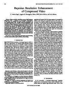
Far-field effects: For miniature arrays, sources are usually located at distances much larger than the distance between recording elements. As a result, the mixing of signals at the recording elements is near singular. Separating independent sources from near ill-conditioned mixtures would require super-resolution signal processing to reliably identify the parameters of the separation manifold. • Near-far effects: For miniature sensor arrays, a stronger source that is closer to the array can mask the signal produced by background sources. Separating the background sources in presence of the strong masker would again require super-resolution processing of the input signals. DSP based source separation algorithms are typically implemented subsequent to a quantization operation (analog-todigital conversion) and hence do not consider the detrimental effects of finite resolution due to the quantizer. In particular, for a high-density sensor array, a naive implementation of a quantizer that uniformly partitions each dimension (pulse coded modulation) of the input signal space could lead to a significant loss of information. To understand the effect of this degradation consider the framework of a conventional source separation algorithm as shown in Fig. 1(a). The “analog” signal x ∈ RM recorded at each of the sensor array is given by x = As, A ∈ RM × RM being the mixing matrix and s ∈ RM being the independent sources of interest. This simplified linear model is applicable to both instantaneous mixing as well as to convolutive mixing formulation [16]. The recorded signals are first digitized and then processed by a digital signal processor (DSP) which implements the source separation algorithm (for example FastICA or SOBI [25]). For the sake of simplicity, assume that the algorithm is able to identify the correct unmixing matrix given by W = A−1 which is then used to recover the source signals ˜s ∈ RM . The effect of quantization in this approach can be captured using a simple additive model as shown in Fig. 1(a) •

˜sd = W(x + q) = s + A−1 q

(1)

where q denotes the additive quantization error introduced during the digitization process. The reconstruction error between the recovered signal ˜sd and the source signal s can then be expressed as ||˜sd − s|| = ||A−1 q|| ≤ ||A−1 ||.||q||

(2)

where ||.|| denotes a matrix and vector norm [23]. Equation (2) indicates that under ideal reconstruction conditions, the performance of conventional source separation algorithm is limited

2

Fig. 1: System architecture where the source separation algorithm is applied (a) after quantization (b) after analog projection and quantization

by: (a) quantization error (accuracy of analog-to-digital conversion) and (b) the nature of the mixing operation determined by A. For high-density sensors, the mixing typically tends to be ill-conditioned (||A−1 || À 1), as a result the reconstruction error due to equation (2) could be large. Now consider the framework shown in Fig.1(b) which is at the core of the proposed resolution enhancement approach. The signals recorded by the sensor array is first transformed by P (in the analog domain) before being quantized. In this case, the reconstructed signal ˜sm ∈ RM can be expressed as ˜sm = D(Px + q).

(3)

For source separation DP = A−1 , for which the reconstructed signal now can be expressed as ˜sm = s + A−1 P−1 q

(4)

which leads to the reconstruction error ||˜sm − s|| = ||A−1 P−1 q|| ≤ ||A−1 P−1 ||.||q||.

(5)

Thus, the reconstruction error can now be controlled by the choice of the transform P and is not completely determined by the mixing transform A. An interesting choice of the matrix P is the one that satisfies ||A−1 P−1 || = 1

(6)

which ensures that the input signals are normalized before processed by the DSP based source separation algorithm. Equation 5 then reduces to ||˜sm − s|| ≤ ||q||

(7)

only if the analog projection P can be precisely and adaptively determined during the process of quantization (“analogto-digital” conversion). This procedure is unlike traditional multi-channel “analog-to-digital” conversion where each signal channel is uniformly quantized the input signal without taking into consideration the spatial statistics of the input signal. Since the projection P is also quantized, the precision to which the condition (6) is satisfied is also important. In this regard, oversampling “analog-to-digital” converters like Σ∆ modulators are attractive since the topology is robust to analog imperfection and can easily achieve dynamic ranges greater than 120 dB (more than 16 bits or accuracy) [20]. In this paper, we extend our work on Σ∆ learning [22] to include theoretical and measurement results obtained for separating sources whose mixtures are near-singular. In particular, we show that the learning algorithm can efficiently and adaptively quantize non-redundant analog signal sub-spaces which leads to significant performance improvement for any DSP based source separation algorithm. The paper is organized as follows: Section II presents a Σ∆ learning framework that estimates the matrix P using an online stochastic gradient algorithm. The algorithm processes samples a continuous time analog signal and produces a sequence of quantized representations that encodes the matrix P and the transformed input signal. We present some of the theoretical properties of the proposed approach and demonstrate the benefits of the approach using representative examples. Section III and IV presents experimental results obtained when the proposed sigma-delta learner interfaces with a conventional ICA module and is used for separating speech samples recorded using a miniature microphone array. Section V concludes with some remarks about the future work in this area. Before we present the Σ∆ learning algorithm in detail we summarize some of the mathematical notations that will be used in this paper. A (bold capital letters) x (normal lowecase letters) x (bold lowecase letters) x[n] ||x||p AT x[n] Ex {.}

En {.}

A Matrix and its elements will be denoted by aij , i = 1, 2, ..; j = 1, 2, ... A Scalar variable. A Vector and its elements will be denoted by xi , i = 1, 2, ... A sequence of vectors where n = 1, 2, .. denotes a discrete time index. The Lp norm of a vector and is given by P ||x||p = ( i |xi |p )1/p . Transpose of A. Discrete time sequences. StatisticalRexpectation and is given by Ex {.} = x (.)px (x)dx, where px (x) denotes the probability density function of x. Empirical expectation and is defined as a temporal average of a discrete time sequence: 1 PN En {dn } = limN →∞ N n=1 d[n].

and the expected performance improvement when employing the framework in Fig. 1(b) over the framework in Fig. 1(a) is given by P I = −20 log ||A−1 ||. (8)

II. O PTIMIZATION F RAMEWORK FOR Σ∆ L EARNING

Equation (8), thus, shows that the for near-singular mixing, ||A−1 || À 1, the performance improvement based on the resolution enhancement technique shown in Fig. 1(b) could be significant. However, the performance improvement is valid

The underlying principle behind the proposed resolution enhancement technique is illustrated using Fig. 2 which shows a two dimensional signal distribution along with the respective signal quantization levels (depicted using rectangular tick

3 C(v)

d[n]

x[n]

+_

+1

d[n]

v[n] +

Q

+

v[n-1] v[n-1]

-1

(a)

(b)

v

(c)

Fig. 4: (a) System architecture of a first order Σ∆ modulator, (b) input-output response of single bit quantizer, and (c) illustration of “limit-cycle” oscillations about the minima of the cost function C(v) Fig. 2: Illustration of the two-dimensional signal distribution for: (a) the input signals ; (b) signals obtained after transformation B and (c) signals obtained after resolution enhancement

marks). In this example, the signal distribution has been chosen to cover only a small region of the quantization space which would be the case for near-singular mixing. Thus, in a traditional implementation where each dimension is quantized independently of the other there would be a significant information loss due to quantization. Our approach towards estimating P while performing signal quantization will be to decompose P ∈ RM × RM as a product two simple matrices Λ ∈ RM × RM and B ∈ RM × RM such that P = ΛB. The transformation matrix B will first “approximately” align the data distribution along the orthogonal axes, each axis representing an independent (orthogonal) component (shown in Fig. 2(b)). Based on this alignment, the signal distribution will be scaled according to a diagonal matrix Λ such that the quantization levels now span a significant region of the signal space (Fig. 2(c)). Our objective will be to compute these transforms B and Λ recursively while performing signal quantization. Even though the proposed procedure bears similarity to recursive techniques reported in many online “whitening” algorithms [15], [16], [13], the key difference for the proposed approach is that the adaptation and estimation of the projection matrix P is coupled with the quantization process. Thus, unlike traditional online “whitening” techniques, in the proposed approach any imperfections or errors in the quantization process can be corrected through the adaptation of P . This approach can therefore be visualized as a “smart” analog-todigital converter as shown in Fig. 3 which not only produces quantized (digitized) representation of the input signal d but also quantized (digitized) representations of the transforms B and Λ. In our formulation, the estimation algorithm for P (B

and Λ) has been integrated within a Σ∆ modulation algorithm and hence the name “Σ∆ learning. The choice of Σ∆ modulation is due to its robustness to hardware level artifacts (mismatch and non-linearity) which makes the modulation amenable for implementing high-resolution analog-to-digital converters [20]. Before we present a generalized formulation for Σ∆ learning we first we first present an optimization framework that can model the dynamics of first-order Σ∆ modulation. A. Stochastic Gradient Descent and Σ∆ Modulators First, we will use a one dimensional example to illustrate how a Σ∆ modulator can be modeled as an equivalent stochastic gradient descent based optimization problem. Consider an architecture of a well known first-order Σ∆ modulator [20] as shown in Fig. 4(a) which consists of a single discrete-time integrator in a feedback loop. The loop also consists of a quantizer Q which produces a sequence of digitized representation d[n], where n = 1, 2, .. denotes a discrete time-index. Let x[n] ∈ R be the sampled analog input to the modulator and without any loss of generality let d[n] ∈ {+1, −1} be the output of a single-bit quantizer given by d[n] = sgn(v[n − 1]) (see Fig. 4(b)) where vn ∈ R is the internal state variable or the output of the integrator as shown in Fig. 4(a). Then, the Σ∆ modulator in Fig. 4(a) implements the following recursion: v[n] = v[n − 1] + x[n] − d[n]

It can be seen from equation (9) that if v[n] is bounded for all n, then N N X 1 X N →∞ 1 d[n] −→ x[n]. (10) N n=1 N n=1 This implies that Σ∆ algorithm given by equation (9) produces a binary sequence d[n] whose temporal average asymptotically converges to the temporal average of the input analog signal. This statistical dynamics is at the core of most Σ∆ modulators. However, from the perspective of statistical learning, the Σ∆ recursion in equation (9) can be viewed as a stochastic gradient step of the following optimization problem: min C(v) = min[|v| − vEx (x)] v

Fig. 3: Architecture of the proposed sigma-delta learning applied to a source separation problem

(9)

v

(11)

where Ex (.) is the ensemble expectation of the random variable x. The optimization function C(v) is shown in Fig. 4(c) for the case |Ex (x)| < 1. The minima under this condition is minv C(v) = 0 which is achieved for v = 0 and thus does not contain any information about the statistical property of

4

1 2

1  K −1    2 K 

2

V 1 K

(a) 2K − 1 2K

1 1   −1 2K 

K −1 K

1

d

2K − 3 2K

Fig. 6: Limit cycle behavior using bounded gradients V 1 K

K −1 K

1

(b) Fig. 5: One dimensional piece-wise linear regularization functions and the multi-bit quantization function as its gradient x. The recursion (9) ensures that v[n] approaches the minima and then exhibits oscillations about the minima (shown in Fig. 4(c)). Note that unlike conventional stochastic gradient based optimization techniques [21], recursion (9) does not require any learning rate parameters. This is unique to the proposed optimization framework where the stochastic gradient descent is used to generate limit-cycles (oscillations) about the minima of the cost function C(v). The only requirement in such a framework is that the assumption that the input signal is bounded which ensures that the limit-cycles are bounded. Under this condition, the statistics of the limit-cycles can asymptotically encode the statistics of the input signal with infinite precision, as shown by equation (10). In the later sections, we will exploit this asymptotic property to precisely estimate the transform P which can then be used for resolving the acute spatial cues in high-density sensor arrays. Another unique aspect of the proposed optimization framework for modeling Σ∆ modulators is that the cost function C(v) links “analog-to-digital” conversion through the regularizer |v| whose derivative leads to a single-bit quantizer (sgn function). The second term in C(v) ensures that the statistics of the quantized stream d[n] matches the statistics of the input analog signal x[n]. We now extend this optimization framework to a multidimensional Σ∆ modulator which uses a multi-bit quantizer and incorporates transformations B and Λ. Consider the following minimization problem min C(v) v

Ω(v) =

M X j=1

|

i vj |; 2K

|vj | ∈ [i − 1, i]

(14)

for i = 1, .., 2K. To reiterate, the uniqueness of the proposed approach, compared to other optimization techniques to solve (12) is the use of bounded gradients to generate Σ∆ limit-cycles. This is illustrated in Fig. 6 showing the proposed optimization procedure using a two-dimensional contour. Provided the input x and the norm of the linear transformation ||B||∞ are bounded and the regularization function Ω satisfies the Lipschitz condition, the optimal solution to (12) is well defined and bounded from below which is shown in the next lemma: Lemma 1: For the bounded matrix ||B||∞ ≤ λ−1 , bounded vector ||x||∞ ≤ 1, C as defined in equation (13) is convex and is bounded by below according to C ∗ = minv C(v) > 1 1 2 ( K − 1). Proof: We will use topological property of norms [23] which states that for two integers p, q satisfying p1 + 1q = 1, the following relationship is valid for vectors v and u |vT u| ≤ ||v||p ||u||q

(15)

(12)

Setting u = Ex {Bx} and applying equation (15) the following inequality is obtained:

(13)

||v||1 ||u||∞ ≥ |vT u| ≥ vT u ≥ vT Ex {Bx}

where the cost function C(v) is given by C(v) = Ω(λ−1 v) − vT Ex {Bx}.

x ∈ RM is now an M dimensional analog input vector and v ∈ RM is an internal state vector. For the first part of this formulation, λ will be assumed to be a constant scalar and the transform B will be assumed to be a constant matrix. Ω(.) denotes a piece-wise linear regularization function that is used for implementing quantization operators. An example of a regularization function Ω(.) is shown in Fig. 5 for 1dimensional input vector v. Due to the piece-wise nature of the function Ω(.) its gradient d = ∇Ω (shown in Fig. 5) is equivalent to scalar quantization operators. Without loss of generality, it will be assumed that the range of the quantization operator is limited between [−1, 1]. Therefore, for a 2K step quantization function the corresponding regularization function Ω(.) is given by

(16)

5

1 It can be easily verified that Ω(v) ≥ ||v||1 − 21 ( K −1) which ¤ is shown graphically in Fig. 5 for a one dimensional case and hence can be extended element-wise to the multi-dimensional Thus, according to Lemma 3, recursion (18) produces a case. quantized sequence whose mean asymptotically encodes the Using the definition of the matrix norm and the given scaled transformed input at infinite resolution. It can also be constraints, it can be easily seen ||B||∞ ≥ ||Bx||∞ ≥ ||u||∞ . shown that for a finite I iterations of (18) yields a quantized Thus, |u||∞ ≤ λ−1 . Therefore, the inequality (16) leads to representation that is log2 (I) bits accurate. 1 1 Ω(λ−1 v)−vT Ex {Bx} ≥ λ−1 ||v||1 − ( −1)−vT Ex {Bx} ≥ 0 2 K B. Σ∆ Learning (17) In this section, we will extend the optimization framework which proves that the cost function C(v) is bounded from to include on-line estimation of the transform B. Here we below by C ∗ . again assume that λ is constant. Given an M dimensional ¤ random input vector x ∈ RM and an internal state vector v, However, for Σ∆ learning the trajectory toward the minima the Σ∆ learning algorithm estimates parameters of a linear M M of the cost function (13) is of importance. A stochastic gradient transformation matrix B ∈ R × R according to the minimization corresponding to the optimization problem (13) following optimization function leads to max(min C(v, B)) (22) v B∈C v[n] = v[n − 1] + Bx[n] − λ−1 d[n] (18) where with n signifying the time steps and d[n] = ∇Ω(v[n − 1]) beC(v, B) = Ω(λ−1 v) − vT Ex {Bx}. (23) ing the quantized representation according to functions shown in Fig. 5. Note also that formulation (18) does not require C denotes a constraint space on the transformation matrix B. any learning rate parameters. As the recursion (18) progresses, The minimization step in equation (22) will ensure that the bounded limit cycles are produced about the solution v∗ (see state vector v is correlated with the transformed input signal Fig. 6) . Bx (tracking step) and the maximization step in (22) will The following two lemma exploits the property of the first- adapt the matrix B such that it minimizes the correlation (deorder modulator to show that the auxiliary state variable v[n] correlation step). defined by (18) is uniformly bounded if the input random The stochastic gradient descent step corresponding to the vector x and matrix B are uniformly bounded. minimization yields the recursion Lemma 2: For any bounded input vector sequence satisfying v[n] = v[n − 1] + B[n]x[n] − λ−1 d[n]. (24) ||x[n]||∞ ≤ 1 and the transformation matrix B satisfying −1 ||B||∞ ≤ λ , the internal state vector v[n] defined by where B[n] denotes the transform matrix obtained at time equation (18) is always bounded, i.e., ||v[n]||∞ ≤ 2λ−1 for instant n. The transform B is then updated according to a n = 1, 2, ... stochastic gradient ascent step given by Proof: We will apply mathematical induction to prove B[n] = B[n − 1] − 2−P v[n − 1]x[n]T ; B[n] ∈ C. (25) this lemma. Without any loss of generality we will assume ||v[0]||∞ ≤ 2λ−1 . Suppose ||v[n − 1]||∞ ≤ 2λ−1 , it then P in equation (25) is a parameter which determines the follows that ||v[n − 1] − ∇Ω(v[n − 1])||∞ = ||v[n − 1] − resolution of updates the parameter matrix B. If we assume d[n]||∞ ≤ λ−1 . Because x and B are bounded and using that locally the matrix B∗ behaves as a positive definite matrix, equation (18), the following relationship holds equation (25) can be rewritten as ||v[n]||∞ = ||v[n − 1] − λ−1 d[n] + Bx[n]||∞ B[n] = B[n − 1] − 2−P v[n − 1](B[n]x[n])T ≤ ||v[n − 1] − λ−1 d[n]||∞ + ||B||∞ T = B[n − 1] − 2−P d[n]d[n] (26) ≤ 2λ−1 (19) where we have replaced the transformed input B[n]x[n] by its ¤ asymptotic quantized representation d[n]. Similarly we have Lemma 3: For any bounded input vector ||x||∞ ≤ 1 replaced v[n − 1] by its quantized representation d[n]. The and bounded transformation matrix B, d[n] asymptotically update can be generalized further by incorporating non-linear n→∞ quantization function φ(.) as satisfies estimates E {d[n]} −→ λE {Bx[n]}. n

n

Proof: Following N update steps the recursion given by equation (18) yields 1 (20) Bx[n] − λ−1 En {d[n]} = (v[N ] − v[0]) N which using the bounded property of random vector v asymptotically leads to n→∞

En {d[n]} −→ λEn {Bx[n]}

(21)

B[n] = B[n − 1] − 2−P φ(d[n])d[n]T

(27)

where φ : RM → RM are functions dependent on the transformation B. Here, we have chosen φ(.) = tanh(.) and the constraint space C has been chosen to restrict B to be a lower triangular matrix with all diagonal elements to be unity. One of the ways to ensure that B[n] ∈ C ∀n is to apply the updates only to lower triangular elements bij ; i > j. The

6

choice of this constraint guarantees convergence of the Σ∆ learning by ensuring B is bounded. Lemma 4: If the transform matrix B is bounded then the quantized sequences di [n] and dj [n] with i 6= j are uncorrelated with respect to each other.

2 (a)

−2

Proof: Using equation (27) the following relationships are obtained: =

B[n] − B[n − 1] B[N ] −2−P En {d[n]φ(d[n])T } = lim N →∞ N En {di [n]φ(dj [n])} = 0 ∀i 6= j (28) Since this relationship holds for a generic form of φ(.), the sequences di [n] are (non-linearly) uncorrelated with respect to each other. ¤ Equation (28) also provides a mechanism of reconstructing the input signal using the transformed output d[n] and the n→∞ converged estimate of the transformation matrix B[n] −→ B∞ . The input signal can be reconstructed using ˆ= x

−1 B−1 En {d[n]}. ∞λ

(29)

The use of lower-triangular transforms for B greatly simplifies the computation of the inverse B−1 ∞ through use of backsubstitution techniques. Also, due to its lower-triangular form, the inverse of B∞ always exists and is well defined. C. Resolution Enhancement Once the transform B has been determined such that the output of the Σ∆ learner is “de-correlated”, we can apply resolution enhancement by “zooming” into the transformed signal space that does not cover the quantization regions (see Fig. 2(b)). This can be achieved using another diagonal matrix Λ−1 which scales each axes as shown in the illustration 2(c). The Σ∆ cost function can be appropriately transformed to include the diagonal matrix Λ ∈ RM × RM as C(v, B, Λ) = Ω(Λ−1 v) − vT Ex {Bx}.

(30)

where the optimization (23) is also performed with respect to the parameter matrix Λ such that the constraint ||B||∞ < ||Λ−1 ||∞ is satisfied. This constraint is to ensure that C(v, B, Λ) is always bounded from below. The stochastic gradient step equivalent to recursion (24) is given by v[n] = v[n − 1] + (B[n − 1]x[n] − Λ−1 [n]d[n])

(31)

The asymptotic behavior of update (31) for equation (30) n→∞ can be expressed as En {d[n]} → ΛEn {Bn xn }. Thus, reducing the magnitude of diagonal elements of Λ will result in an equivalent amplification of the transformed signal. To satisfy the constraint on the transform B and Λ, a suitable update for the diagonal matrix Λ and its elements λi are λi = max |(B[n]x[n])i |; N1 > n > N0

(32)

where N0 is the number of iterations required for the matrix B to stabilize and N1 is the maximum observation period used to determine the parameters λi .

0

500

1000

1500

2000

0

500

1000

1500

2000

0

500

1000

1500

2000

0

500

1000

1500

2000

2 (b)

−2−P d[n]φ(d[n])T

0

0 −2 2

(c)

0 −2 2

(d)

0 −2

Fig. 7: Reconstruction of the sources using conventional and proposed Σ∆ with OSR=1024

III. N UMERICAL E VALUATION OF Σ∆ L EARNING We first verify the improvement achievable using Σ∆ learning as predicted by the equations (8). For this controlled experiment we have chosen two synthetic signals which have been also used in previous studies [24]. s1 (t) = 480t − b480tc s2 (t) = sin(800t + 6 cos(90t))

(33)

Each of these source signals were mixed using a random illconditioned matrix A to obtain the two-dimensional signals which were then processed by the Σ∆ learner. The outputs of the Σ∆ learner were then used to reconstruct the source signals according to ˜sd ˜sm ˜sm ´

= A−1 x −1

−1

= A B x = A−1 B−1 Λ−1 x

(34) (35) (36)

assuming that the un-mixing matrix A−1 can be perfectly determined. The equations (34)- (36) represent the following three cases: (a) ˜sd which is the signal reconstructed using a Σ∆ modulator without any learning (denoted by without); (b) ˜sm which is the signal reconstructed using Σ∆ learning without resolution enhancement (denoted by with); and (c) ˜sm ´ which is the signal reconstructed using Σ∆ learning with resolution enhancement (denoted by with+). For this experiment, the condition number of the mixing matrix was chosen to be 1000 and the oversampling ratio (OSR), which is defined as the sampling frequency/Nyquist frequency, was chosen to be 1024. For the signal in (33) the Nyquist frequency was chosen to be 10 KHz. Figure 7 shows the reconstructed signals obtained with and without the application of Σ∆ learning. The quantization artifacts can be clearly seen Fig. 7(b) which is the signal recovered using Σ∆ modulator without learning. However, the signals obtained when Σ∆ learning is applied does not show any such artifacts indicating improvement in resolution. To quantify this improvement, we compared the signal-to-error

7

25

without with with+

15 Signal to Error Ratio (dB)

Signal to Error Ratio (dB)

20

15

10

5

SER = log2 {

10

5

0

0

−5

ratio (SER) for the separated signals. SER is defined as

20 without with with+

5

6

7 8 9 Log (OSR)

−5

10

5

6

2

7 8 9 Log (OSR)

10

2

(a)

(b)

Fig. 8: Evaluating the reconstruction of the sources for classical (without), learning (with), and learning with resolution enhancement (with+) Σ∆ at different OSR for log2 (condition number) of (a) 10 and (b) 12 30

30 without with with+

20 15 10 5

20

15

10

5

0 −5

without with with+

25 Signal to Error Ratio (dB)

Signal to Error Ratio (dB)

25

6

7 8 9 10 11 12 Log (Condition number) 2

0

6

7 8 9 10 11 12 Log (Condition number) 2

(a)

(b)

Fig. 9: Evaluating the reconstruction of the sources for classical (without), learning (with), and learning with resolution enhancement (with+) Σ∆ at different condition number for OSR of (a) 256 and (b) 512

25 2 Dim 3 Dim 6 Dim

Signal to Error Ratio (dB)

20

15

10

5

0

6

7 8 9 10 11 12 Log (Condition number) 2

Fig. 10: Evaluating the reconstruction of sources at different dimension for the learning Σ∆ at different condition number for OSR of 128

||s||2 } ||s − ˜s||2

(37)

where s and ˜s is based on the definition in (34)- (36). To compute the mean SER and its variance 10 different mixing matrices with a fixed condition number were chosen and the mean/variances were calculated across different experimental runs. Fig. 8(a) compares the SER obtained when the mixing matrix with condition number 210 was chosen for different values of OSR. Figure 8(b) compares the SER obtained when the mixing matrix with condition number 212 was chosen. It can be seen in Fig. 8(a) and (b) that as the OSR of the Σ∆ modulator increases, the SER increases. This is consistent with results reported for Σ∆ modulators where OSR is directly related to the resolution of the “analog-to-digital” conversion. However, it can be seen that for all conditions of OSR, Σ∆ learning with resolution enhancement outperforms the other two approaches. Figure 9(a) and (b) compares the performance of Σ∆ learner when the condition number of the mixing matrix is varied for fixed over-sampling ratios of 256 and 512. The results again show that Σ∆ learner (with and without resolution enhancement) demonstrates consistent performance improvement over the traditional Σ∆ modulator. Also, as expected the SER performance for all the three cases deteriorates with the increasing condition number, which indicates that the mixing becomes more singular. Figure 10 evaluates the SER achieved by Σ∆ learning (with resolution enhancement) when the dimensionality of the mixing matrix is increased. For this experiment, the number of source signals are increased by randomly selecting signals which were mutually independent with respect to each other. It can be seen from Fig. 10 that the response of the Σ∆ learning is consistent across different signal dimensions with larger SER when the dimension is lower. In the next set of experiments the performance of Σ∆ learning is evaluated for the task of source separation when the un-mixing matrix is estimated using an ICA algorithm. Speech samples were obtained from TIMIT database and were synthetically mixed using an ill-conditioned matrix with different condition number. The instantaneous mixing parameters are shown in Fig. 11 which simulates the “near-far” scenario where one of the speech sources is assumed to be much closer to the microphone array than the other. This scenario was emulated by scaling one of the signals by −50dB with respect to another, as shown in Fig. 11. The speech mixture is then presented to the Σ∆ learner and its output is then processed by a second-order blind inference (SOBI) [25] and by an efficient FastICA (EFICA) [26] algorithms. The performance metrics chosen for this experiment is based on source-todistortion ratio (SDR) [27] where the estimated signal sˆj (n) is decomposed into sˆj (n) = starget (n) + einterf (n) + eartif (n)

(38)

with starget (n) being the original signal, and einterf (n) and eartif (n) denote the interference and artifacts errors, respectively. The SDR metric is a global performance metric which

8

20

20

15

15

10

10

5

5 SDR (dB)

SDR (dB)

Fig. 11: Source signals s1 and s2 (subplots a and b) and mixed signals x1 and x2 (subplots c and d).

0 −5 −10

0 −5

2d

−10 with (S1) with (S2) without (S1) without (S2)

−15 −20 −25

si

6

7

8 9 10 Log (OSR) 2

(a)

11

12

with (S1) with (S2) without (S1) without (S2)

−15 −20 −25

6

7

8 9 10 Log (OSR)

11

12

xj

pj ui

2

(b)

Fig. 12: SDR corresponding to with/without Σ∆ learning for the near-far recording conditions illustrated in Fig 11 using (a) SOBI and (b) EFICA algorithms. then measures both source-to-interference ratio (SIR) - the amount of interferences from non wanted sources and also other artifacts like quantization and musical noise. The SDR is defined as: kstarget k2 SDR = 10 log (39) keinterf + eartif k2 The speech sources s1 and s2 in Fig. 11 consists of 44200 samples with a sampling rate of 16KHz which is also the Nyquist rate. Figure 11 also shows that, after mixing, one of the sources is being completely masked by the other which is consistent with the“near-far” effect. Figure 12(a) and (b) shows the SDR obtained using the Σ∆ learning when the OSR is varied from 128 to 4096 . Also shown in Fig. 12 (a) and (b) are the SDR metrics obtained when a conventional Σ∆ algorithm is used. It can be seen from the Fig. 12 that the SDR corresponding to the stronger source is similar for both cases (with and without Σ∆ learning), where as for the masked source the SDR obtained using Σ∆ learning is superior. This is consistent with the results published in [28]. However, the approach in [28] is applied after quantization

Fig. 13: Far-field recording using a two-element sensor array

and hence according to formulation in section I, is limited by the condition number of the mixing matrix. It should also be noted that the Σ∆ learning only enhances the resolution of the measured signals. The ability to successfully recover the weak source under “near-far” conditions, however, is mainly determined by the choice of the ICA algorithm. IV. FAR - FIELD E XPERIMENTS USING M INIATURE M ICROPHONE A RRAYS In this section we first present a mathematical model for a miniature microphone array and show that the recorded signals from the array can be near singular. Then, we use this model with the Σ∆ learner to compare the performance of the algorithm with a traditional source separation technique. We then verify the proposed approach using speech data collected using a prototype miniature microphone array under real recording conditions. A. Far-field model for a miniature microphone array We illustrate a specific instance of singular mixing that occurs in the case of miniature microphone arrays. For this

9

10

1cm

0

5 0

S1

−5

x

−10 −15 −20

SDR (dB)

SDR (dB)

o

0 SDR (dB)

−5

S4

z

5

5

S3 S2

10

−5

−10 −15

−10 −20

−25

y

with without

−30 −35

6

7 8 9 Log2(OSR)

(a)

10

−15

−20

(b)

with without 6

7 8 9 Log2(OSR)

10

−25 −30

with without 6

7 8 9 Log2(OSR)

(c)

10

(d)

Fig. 14: Σ∆ performance with and without learning for three speech signals corresponding to the far-field model

modeling we resort to the far-field wave propagation models that have been extensively studied within the context of plenacoustic signal processing [17]. For modeling purposes, consider a sensor array shown in Fig. 13 that consists of two recording elements. If the inter-element distance is much less than the wavelength of the sensor signal of interest, the signals recorded at each of the sensor elements can be approximated using far-field models. Also, for miniature sensor array the distance to the sources from the center of the array can be assumed to be larger than the inter-element distance. We express the signal xj (pj , t) recorded at j th sensor as a superposition of i independent sources si (t) (i ∈ 1, .., D), each of which are referenced with respect to the center of the array [17]. This can be written as X xj (pj , t) = ci (pj )si (t − τi (pj )) (40) i

where ci (pj ) and τi (pj ) denotes the attenuation and delay, for the source si (t) at the position pj , measured relative to the center of the sensor array. pj in equation (40) denotes the position vector of the j th microphone. Equation (40) can be approximated using Taylor’s series expansion as

xj (pj , t) =

X

ci (pj )

i

∞ X (−τi (pj ))k

k!

k=0

(k)

si (t)

(41)

Under far-field conditions it can be assumed that ci (pj ) ≈ ci is constant across all the sensor elements. Also, the higherorder terms in the series expansion (41) can be ignored and can be expressed as X X xj (pj , t) ≈ ci si (t) − ci τi (pj )s˙ i (t). (42) i

P

i

The component xc (t) = i ci si (t) signifies the commonmode signal common to all the recording elements and the second part of the RHS signifies an instantaneous mixture of the derivative of the source signals. The common-mode component can be canceled using a differential measurement [18]

under which equation (42) becomes ∆xj (pj , t) = xj (pj , t) − xc (t) ≈ −

X

ci τi (pj )s˙ i (t) (43)

i

and can be expressed in a matrix-vector form as ∆x(t) ≈ −A˙s(t)

(44)

where A = {ci τi (pj )} denotes the instantaneous mixing matrix. Under far-field approximation, the time delays can be expressed as τi (pj ) = uTi pj /v (45) where ui is the unit normal vector of the wavefront of source i and v is the speed of sound (v = 340m/s in air). Thus equations (44) and (45) show that for miniature recording array, recovery of the desired sources s or s˙ entails solving a linear source separation problem [19]. However, equation (45) reveals that sources that are located closer to the sensor array can completely mask the sources located away from the sensor array, resulting in a near-singular mixing A. As shown in the following description that under near-singular mixing conditions, conventional methods of signal acquisition and source separation fail to deliver robust performance. B. Experiments with Far-field Model In this setup, we simulated recording conditions that consisted of four closely spaced microphones. The arrangement is shown in Fig. 14(a) where each circle represents a microphone of dimension 1cm. In this arrangement, three of the microphones were placed along a triangle, whereas the fourth microphone was placed at the centroid and act as the reference sensor which records the common signal. The set up is similar to the conditions that have been reported in [19] where the simulation have been shown to be consistent with recording in the real-life conditions. The outputs of each microphone along the triangle were subtracted from the reference microphone to produce three differential outputs. In our experiments we used three independent speech signals as

8000

8000

6000

6000

Frequency

Frequency

10

4000 2000 0

0.5

2000

8000

1 Time (c)

1.5

Frequency

2000 1 Time (e)

1.5

2

0.5

1 Time (d)

1.5

2

0.5

1 Time (f)

1.5

2

4000 2000

8000

4000

0.5

1 Time (b)

6000

0

2

6000

0

0.5

8000

4000

0.5

2000 0

2

6000

0

Frequency

1.5

Frequency

Frequency

8000

1 Time (a)

4000

1.5

2

6000 4000 2000 0

Fig. 15: Spectrogram of the recorded signals (subplots (a) and (b)) and recovered signals using Σ∆ without learning (subplots (c) and (d)) and with learning (subplots (e) and (f))

far-field sources. The differential outputs of the microphone array were first presented to the proposed Σ∆ learner, and the outputs of Σ∆ learner array were then used as inputs to the SOBI algorithm. A benchmark used for comparative study consisted of Σ∆ converters that directly quantized the differential outputs of the microphones. Figure 14(b)-(d) summarizes the performance of source separation (with and without Σ∆ learning) for different orientation of the acoustic sources. For the three experiments, only the bearing of the sources were varied but their respective distances to the center of the microphone was kept constant. It can be seen that for each of these orientations, source separation algorithm that uses Σ∆ learning as a front-end “analog-to-digital” converter delivers superior performance compared to the algorithm that does not use Σ∆ learning. Also, from Fig. 14(b)-(d) it can be seen that the improvement in SDR performance significantly increases when the sampling frequency (resolution) decreases showing that Σ∆ learning efficiently utilizes the available resolution (due to coarse quantization) to capture information necessary for source separation. C. Experiments with real microphone recordings In this set of experiments, we have applied Σ∆ learning to speech data that was recorded using a prototype miniature microphone array, similar to the set up described in [18]. The four omni-directional microphones Knowles FG3629 were mounted on a circular array with radius 0.5 cm. The differential microphone signals were pre-processed using secondorder bandpass filters with low-frequency cutoff at 130 Hz

and high-frequency cutoff at 4.3 kHz. The signals were also amplified by 26dB. The speech signals were presented through loudspeakers positioned at 1.5 m distance from the array and the sampling frequency of the National Instruments data acquisition card was set to 32 KHz. Male and female speakers from TIMIT database were chosen as sound sources and was replayed through standard computer speakers. The data was recorded from each of the microphones, archived, and then presented as inputs to the Σ∆ learning and the SOBI algorithm. Figure 15(a) and (b) shows the spectrogram of the speech signals recorded from the microphone array. The two spectrograms look similar, thus emulating a “near-far” recording scenario where a dominant source masks the background weak source. Also it can be seen from the spectrogram in Fig. 15(b) that one of the recordings is more noisy than the other (due to microphone mismatch). Figure 15(c) and (d) show the spectrogram of the separated speech signals obtained without Σ∆ learning. Figure 15(e) and (f) show the spectrogram of the separated speech signals obtained with Σ∆ learning. A visual comparison of the spectrograms show that separated speech signal (without Σ∆ learning) contain more quantization artifacts which can be seen as the broadband noise in Fig. 15(c) and (d). The table I summarizes the SDR performance (for different OSR) for each of the sources in these two cases (with and without Σ∆ learning), showing that Σ∆ learning indeed improves the performance of the source separation algorithm. Also, from table I, it can be seen that when the OSR increases, the performance differences between

11

TABLE I: Performance (SDR (dB) ) of the proposed Σ∆ for the real data for different over-sampling ratio. OSR=4

S1 S2

OSR=8

OSR=16

OSR=32

OSR=64

with

without

with

without

with

without

with

without

with

without

1.03 -12.52

-0.72 -13.15

1.33 -9.77

0.41 -10.17

1.34 -8.69

0.94 -8.88

1.3 -8.29

1.15 -8.32

1.28 -8.12

1.21 -8.1

the two cases becomes insignificant. This artifact is due to the limitations in the SOBI algorithm for separating sources with high fidelity, noise in the microphones and ambient recording conditions. V. C ONCLUSIONS AND D ISCUSSIONS In this paper, we have argued that the classical approach of signal quantization followed by DSP based source separation fails to deliver robust performance when processing signals recorded using miniature sensor arrays. We proposed a framework that combined statistical learning with Σ∆ modulation and can be used for designing “smart” high-dimensional analog-to-digital converters that can exploit spatial correlations to resolve acute differences between signals recorded by miniature sensor array. Even though in this paper Σ∆ learning has been demonstrated to improve the performance of speech based source separation algorithms, the proposed technique is general and can be applied to any sensor array. The potential applications include microphone array hearing aids, microelectrode array in neuroprosthetic devices, miniature radio-frequency antenna arrays and for radar applications. The experimental results presented in this paper demonstrated that the Σ∆ learning algorithm consistently led to a superior performance over the classical approach and hence is attractive for implementing high-dimensional analog-to-digital converters. The future work in this area will include: (a) exploring higher-order noise-shaping Σ∆ modulators for improving the performance of resolution enhancement; (b) extending Σ∆ learning to non-linear signal transforms by embedding kernels into the optimization framework; (c) extending Σ∆ learning to integrate ICA with signal quantization. ACKNOWLEDGMENT The authors would like to thank the Prof. Milutin Stancevic from Stony Brook University for providing us with the real microphone data to which we have applied the Σ∆ learning algorithm. This work was supported in part by a grant from the National Science Foundation (IIS:0836278). R EFERENCES [1] M.J. Madou, M.J., Fundamentals of Microfabrication: The Science of Miniaturization, Boca Raton, FL: CRC Press, 2002. [2] K.D. Wise, D.J. Anderson, J.F. Hetke, D.R. Kipke, and K. Najafi, “Wireless implantable microsystems: High-density electronic interfaces to the nervous system,” Proceedings of the IEEE, vol. 92, no. 1, pp. 138-145, Jan. 2004. [3] C.T. Nordhausen, E.M. Maynard, and R.A. Normann, “Single unit recording capabilities of a 100-microelectrode array,” Brain Research, vol. 726, pp. 129-140, 1996. [4] K.D. Wise and K. Najafi, “Microfabrication techniques for integrated sensors and microsystems,” Science, vol. 254, pp. 1335-1342, Nov. 1991.

[5] R.N. Miles and R.R. Hoy, “The development of a biologically-inspired directional microphone for hearing aids,” Audiology and Neuro-Otology, vol. 11, no. 2, pp. 86-94, 2006. [6] J.E. Greenberg and P.M. Zurek, “Microphone array hearing aids in microphone arrays: Signal Processing Techniques and Application,” Springer, Berlin, pp. 229-253, 2001. [7] B. Edwards, “The future of hearing aid technology,” Trends in Amplification, vol. 11, no 1, pp. 31-45, Mar. 2007. [8] C. Jutten and J. H´erault, “Blind separation of sources, Part 1: an adaptive algorithm based on neuromimetic architecture,” Signal Processing, vol. 24, no. 1, pp. 1-10, July 1991. [9] A. Hyv¨arinen, J. Karhunen, and E. Oja, Independent Component Analysis, New York: Wiley, 2001. [10] A. Hyv¨arinen and E. Oja, “Independent component analysis: Algorithms and applications,” Neural Networks, vol. 13, pp. 411-430, 2000. [11] P. Comon, “Independent component analysis - a new concept?,” Signal Processing, vol. 36, pp. 287-314, 1994. [12] A.J. Bell and T.J. Sejnowski, “An Information-Maximization Approach to Blind Separation and Blind Deconvolution,” Neural Computation, vol. 7, pp. 1129-1159, 1995. [13] S. Amari, A. Cichocki, and H.H. Yang, “A new learning algorithm for blind signal separation,” in Adv. Neural Information Processing Systems (NIPS), vol. 8, pp. 757-763, Cambridge: MIT Press, 1996. [14] J.-F. Cardoso and B.H. Laheld, “Equivariant adaptive source separation,” IEEE Trans. Signal Process., vol. 44, no. 12, pp. 30173030, 1996. [15] E. Oja, “Principal components, minor components, and linear neural networks,” Neural Networks, vol. 5, no. 6, pp.927-935, 1992. [16] A. Cichocki and S. Amari, Adaptive Blind Signal and Image Processing: Learning Algorithms and Applications, New York, NY: Wiley, 2002. [17] M.N. Do, “Toward sound-based synthesis: the far-field case,” in Proc. Int. Conf. Acoustics, Speech and Signal Processing (ICASSP), Canada, 2004. [18] A. Celik, M. Stanacevic, and G. Cauwenberghs, “Gradient flow independent component analysis in micropower VLSI,” Adv. Neural Information Processing Systems (NIPS), vol. 8, pp. 187-194, Cambridge: MIT Press, 2006. [19] J. Barr`ere, and G. Chabriel, “A Compact Sensor Array for Blind Separation of Sources,” IEEE Trans. Circuits and Systems: Part I, vol. 49, no. 5, pp. 565-574, 2002. [20] J.C. Candy and G.C. Temes, “Oversampled methods for A/D and D/A conversion,” in Oversampled Delta-Sigma Data Converters, Piscataway, NJ: IEEE Press, pp. 1-29, 1992. [21] L. Bottou, “Stochastic learning,” in Advanced Lectures on Machine Learning, Lecture Notes in Artificial Intelligence, vol. 3176, O. Bousquet and U. von Luxburg, Ed. Berlin: Springer Verlag, 2004, pp. 146-168. [22] A. Fazel, S. Chakrabartty, “Sigma-Delta resolution enhancement for farfield acoustic source separation,” in Proc. Int. Conf. Acoustics, Speech and Signal Processing (ICASSP), Las Vegas, NV, 2008. [23] W. Rudin, Functional Analysis, New York: McGraw-Hill, 1991. [24] A. Cichocki, R.E. Bogner, L. Moszczynski, and K. Pope, “Modified Hrault-Jutten algorithms for blind separation of sources,” Digital Signal Processing, vol. 7, no. 2, pp. 80-93, 1997. [25] A. Belouchrani, K. Abed-Meraim, J.-F. Cardoso, E. Moulines, “A blind source separation technique using second-order statistics,” IEEE Trans. Signal Process., vol. 45, no. 2, pp. 434444, 1997. [26] Z. Koldovsk´y, P. Tichavsk´y and E. Oja, “Efficient Variant of Algorithm FastICA for Independent Component Analysis Attaining the Cram´er-Rao Lower Bound,” IEEE Trans. on Neural Networks, Vol. 17, No. 5, Sept 2006. [27] E. Vincent, R. Gribonval, and C. Fvotte, “Performance measurement in Blind Audio Source Separation,” IEEE Trans. Audio, Speech, and Lang. Processing, vol. 14, no. 4, pp. 1462-1469, July 2006. [28] M. Gupta and S. C. Douglas, “Performance Evaluation of Convolutive Blind Source Separation of Mixtures of Unequal-Level Speech Signals,” in Proc. Int. Symposium on Circuits and Systems (ISCAS), New Orleans, Louisiana, 2007.

12

Amin Fazel (S’07) received the B.Sc. degree in computer science and engineering from Shiraz University, Shiraz, Iran, in 2002 and the M.Sc. degree in computer engineering from Sharif University of Technology, Tehran, Iran, in 2005. Currently, he is pursuing the Ph.D. degree in electrical and computer engineering at Michigan State University. His research interests include speech processing, robust speech/speaker recognition, acoustic source separation, and analog-to-information converters.

Amit Gore received the B.E. degree in instrumentation engineering from the University of Pune, Pune, India, in 1998, and the M.S. and Ph.D. degrees in electrical and computer engineering from Michigan State University, East Lansing, in 2002 and 2008, respectively. Currently, he is with General Electric Global Research, Niskayuna, New York. His research interests are low-power sigma-delta converters, analog signal processing and low-power mixed-signal VLSI design.

Shantanu Chakrabartty (M’96-SM’09) received his B.Tech degree from Indian Institute of Technology, Delhi in 1996, M.S and Ph.D in Electrical Engineering from Johns Hopkins University, Baltimore, MD in 2001 and 2004 respectively. He is currently an assistant professor in the department of electrical and computer engineering at Michigan State University. From 1996-1999 he was with Qualcomm Incorporated, San Diego and during 2002 he was a visiting researcher at University of Tokyo. His current research interests include low-power analog and digital VLSI systems, hardware implementation of machine learning algorithms with application to biosensors and biomedical instrumentation. Dr. Chakrabartty was a recipient of The Catalyst foundation fellowship from 19992004 and received the best undergraduate thesis award in 1996. He is currently a member for IEEE BioCAS technical committee, IEEE Circuits and Systems Sensors technical committee and serves as an associate editor for Advances in Artificial Neural Systems from Hindawi publications.