dler and Zang [HZ80] and Beasley and Christofides [BC89] is the solution of a linear programming ..... John Wiley & Sons, Inc, 1998. [CMS93] K. Clarkson, K.
Resource Constrained Shortest Paths ? Kurt Mehlhorn1 and Mark Ziegelmann1?? Max-Planck-Institut f¨ur Informatik, Stuhlsatzenhausweg 85, 66123 Saarbr¨ucken, Germany, mehlhorn,mark �mpi-sb.mpg.de http://www.mpi-sb.mpg.de/~ mehlhorn,mark
f
g
f
g
Abstract. The resource constrained shortest path problem (CSP) asks for the computation of a least cost path obeying a set of resource constraints. The problem is NP-complete. We give theoretical and experimental results for CSP. In the theoretical part we present the hull approach, a combinatorial algorithm for solving a linear programming relaxation and prove that it runs in polynomial time in the case of one resource. In the experimental part we compare the hull approach to previous methods for solving the LP relaxation and give an exact algorithm based on the hull approach. We also compare our exact algorithm to previous exact algorithms and approximation algorithms for the problem.
1 Introduction The resource constrained shortest path problem (CSP) asks for the computation of a least cost path obeying a set of resource constraints. We are given a graph G = (V; E ), a source node s and a target t, and k resource limits λ(1) to λ(k) . Each edge e has a cost ce (i) and uses re units of resource i, 1 � i � k. Cost and resource usages are assumed to be non-negative. They are additive along paths. The goal is to find a least cost path from s to t satisfiying the resource constraints. CSP has applications in mission planning and operations research. CSP is NP-complete even for the case of one resource [HZ80]. The problem has received considerable attention in the literature [Jok66, Han80, HZ80, AAN83, MR85, Hen85, War87, BC89, Has92, Phi93]. The first step in the exact algorithms of Handler and Zang [HZ80] and Beasley and Christofides [BC89] is the solution of a linear programming relaxation. Hassin [Has92] gives a pseudo-polynomial algorithm for one resource that runs in time O(nmC) for integral edge costs from the range [0 :: C℄. He also gives an ε-approximation algorithm that runs in time O(nm=ε). Other approximation algorithms were given by Phillips [Phi93]. In our experiments the approximation algorithm of Hassin was much slower than our exact algorithm. We discuss the previous work in more detail in later sections of the paper. In the theoretical part of our paper we study a linear programming relaxation of the problem. It was studied before by Handler/Zang [HZ80] and Beasley/Christofides [BC89] who obtained it by Lagrangean relaxation of the standard ILP formulation. The latter ? ??
An extended version of this paper is available at http://www.mpi-sb.mpg.de/~mark/r sp.ps Supported by a Graduate Fellowship of the German Research Foundation (DFG).
authors use a subgradient procedure to (approximately) solve the LP and the former authors gave a combinatorial algorithm for solving the LP in the case of one resource. We give a new geometric interpretation of their algorithm and use it to extend the algorithm to the case of many resources. We also show the polynomiality of the algorithm in the case of one resource: the LP can be solved by O(log(nRC)) shortest path computations. This assumes that the ce and re are integral and contained in the ranges [0 :: C℄ and [0 :: R℄, respectively. Polynomiality of the algorithm in the case of many resources stays open. It follows from the Ellipsoid method that the LP can be solved in polynomial time for any number of resources. In the experimental part we first compare the hull approach to solving the relaxation with the subgradient method of Beasley/Christofides that approximately solves the Lagrangean relaxation. The hull approach is simultaneously more efficient and more effective in the single resource case; it gives better bounds in less time. For many resources the relation is less clear. In Section 3 we describe an exact algorithm that follows the general outline of the algorithms of Handler/Zang and Beasley/Christofides and works in three steps: (1) Compute a lower bound LB and an upper bound UB for the objective value by either the hull approach or the subgradient procedure. (2) Use the results of the first step to prune the graph, i.e. to delete nodes and edges which cannot possibly lie on an optimal path. (3) Close the gap between lower and upper bound by enumerating paths. We use the methods of Beasley/Christofides for the second step. The fact that the hull approach gives better bounds than the subgradient procedure makes pruning more effective. Finally, we discuss three methods for gap closing: (1) Applying the pseudopolynomial algorithm of Hassin [Has92] to the reduced graph. (2) Enumerating paths in order of increasing reduced cost (the cost function suggested by the optimal solution of the LP) as suggested by Handler and Zang using the k-shortest path algorithm of [JM99]. (3) Enumerating paths in order of increasing reduced cost combined with on-line pruning. This method is new. Our new method turns out to be most effective in the single resource case when the number of paths to be ranked is large (it otherwise gives similar results as the second method, whereas the first method is only efficient when the pruning reduced the graph drastically). However, the path ranking via k-shortest paths usually outperforms our new method in the multiple resource case. In our experiments we used random grid graphs, digital elevation models, and road graphs. For all three kinds of graphs the running time of the third step is small compared to that of the first two steps for the single resource case and hence the observed running time of our exact algorithm is O(m + n logn) � log(nCR). This compares favorably with the running time of the pseudo-polynomial algorithm (O(nmC)) and the approximation algorithm (O(nm=ε)) of Hassin. It is therefore not surprising that the latter algorithms were not competitive in our experiments.
2 Relaxations We start with a (somewhat unusual) ILP formulation. For any path p from s to t we (i) introduce a 0-1 variable x p and we use c p and r p (i = 1; : : : ; k) to denote the cost and
X X X
resource consumption of p, respectively. Consider min
cpxp
(1)
xp = 1
(2)
p
s.t.
p
r p x p � λ(i) (i)
i = 1; : : : ; k
(3)
p
x p 2 f0; 1g
(4)
This ILP models CSP. Observe that integrality together with (2) guarantees that x p =1 for exactly one path, (3) ensures that this path is feasible, i.e. obeys the resource constraints, and (1) ensures that the cheapest feasible path is chosen. We obtain an LP by dropping the integrality constraint. The objective value LB of the LP relaxation is a lower bound for the objective value of CSP. The linear program has k + 1 constraints and an exponential number of variables and is non-trivial to solve. Beasley/Christofides approximate LB from below by relaxing the resource constraint in a Lagrangean fashion and using subgradient optimization to approximately solve the Lagrangean relaxation1. The dual of the LP has an unconstrained variable u for equation (2) and k variables vi � 0 for the inequalities (3): The dual problem can now be stated as follows: max u + λ(1)v1 + ��� + λ(k) vk
s.t. u + r p v1 + ��� r p vk � c p i = 1; : : : ; k vi � 0 (1)
(k)
(5)
8p
(6) (7)
The dual has only k + 1 variables albeit an exponential number of constraints. Lemma 1. The dual can be solved in polynomial time by the Ellipsoid Method. Proof. Let u� ; v�1 ; : : : ; v�k be the current values of the dual variables. The separation prob(1) lem amounts to the question whether there is a path q such that u� + v�1 rq + ��� + ( k ) ( 1 ) ( k ) v�k rq > cq or equivalently cq v�1 rq ��� v�k rq < u� : This question can be solved
with a shortest path computation with the scaled edge costs c˜e = ce v1 re ��� (k) vk re . Hence we can identify violated constraints in polynomial time which completes the proof. (1)
1
�
P
�
P P
For any v 0 the linear program min p (c p + v(λ r p )) subject to x 0 and p x p = 1 is easily solved by a shortest path computation (with respect to the edge costs ce vre ) and is a lower bound for LB (this is obvious in the presence of the additional constraint p r p x p λ; dropping the constraint can make the minimum only smaller). Subgradient optimization uses an iterative procedure to approximate the value of v which maximizes the bound. In general, the maximum is not reached, but only approximated. It is known (see, for example, [CCPS98]) that the maximum is equal to the objective value of the LP relaxation.
�
2.1 The Single Resource Case The dual now has two variables, u and v � 0 and can be interpreted geometrically. Standard Interpretation [HZ80]: A pair (u; v) is interpreted as a point in the u-vplane. Each constraint is viewed as a halfspace in the u-v-plane and we search for the maximal feasible point in direction (1; λ) (see Figure 1).
u
c
direction (1; λ)
r v
λ
Fig. 1. (left) Find maximal point in direction (1; λ) in the intersection of halfspaces. (right) Find line with maximal c-value at r = λ which has all points above or on it.
(Geometric) Dual Interpretation: A pair (u; v) is interpreted as a line in r-c-space (the line c = vr + u). A constraint u + r p v � c p is interpreted as a point (r p ; c p ) in r-cspace. Hence every path corresponds to a point in r-c-space. We are searching for a line with non-positive slope that maximizes u + λv while obeying the constraints, i.e. which has maximal c-value at r = λ, and which has all points (r p ; c p ) above or on it (see Figure 1), i.e., we are searching for the segment of the lower hull2 which intersects the line r = λ. We now use the new interpretation to derive a combinatorial algorithm for solving the dual. Although equivalent to Handler/Zang’s method, our formulation is simpler and more intuitive. The hull approach: We are searching for the segment of the lower hull which intersects the limit line r = λ. We may compute points on the lower hull with shortest path computations, e.g. the extreme point in c-direction is the point corresponding to the minimal length path and the extreme point in r-direction is the point corresponding to the minimal resource path. We start with the computation of the minimum resource path. If this path is unfeasible, i.e. all points lie to the right of the limit line, the dual LP is unbounded and the CSP problem is unfeasible. Otherwise we compute a lower bound, the minimum length path. If this path is feasible, we have found the optimum of CSP, the constraint λ is redundant in that case. Otherwise we have a first line through the two points that corresponds to a (u; v)value pair where v is the slope and u the c-abscissae of the line. 2
We use a sloppy definition of lower hull here: there is a horizontal segment to the right incident to the lowest point.
Now we test whether all constraints are fulfilled, i.e. whether all points lie above or on the line. This separation problem is solved with a shortest path computation with the scaled costs c˜e = ce vre and can be viewed as moving the line in its normal direction until we find the extreme point in that direction (see Figure 2). If no point below the
c prmin
pcmin
r λ Fig. 2. Finding a new point on the lower hull
line is found, we conclude that no constraint is violated and have found the optimal line. The optimal value of the dual relaxation is its intersection with the limit line r = λ. Otherwise we update the line: The new line consists of the new point and one of the two old points such that we again have a line that has all previously seen hull points above it and that intersects the limit line with maximal c-value. We iterate this procedure until no more violating constraint is found. The Simplex Approach: It is also possible to interpret the hull approach as a dual simplex algorithm with cutting plane generation. We maintain the optimum for a set of constraints. New constraints are generated solving the separation problem with a shortest path computation. The dual simplex algorithm is used to find the optimum for the new set of constraints which is possible in a single pivot step. See the extended version for further details. 2.2 Running time of the hull approach Now we show that the number of iterations to solve the dual relaxation for integral lengths and resources is logarithmic in the input. This is the first result that gives nontrivial bounds for the number of iterations 3 . We assume that edge costs and resources are integers in the range [0::C℄ and [0::R℄, respectively. This implies that the cost and resource of a path lie in [0::nC℄ and [0::nR℄, respectively. 3
Anderson and Sobti [AS99] give an algorithm for the table layout problem that works similarly to the hull approach solving parametrized flow problems in each iteration. Using a simple modification of our proof it is also possible to show a logarithmic bound on the number of iterations in their case.
Theorem 1. The number of iterations of the hull approach is O(log(nRC)). Hence the relaxed problem CSPrel can be solved in O(log(nRC)(n log n + m)) time which is polynomial in the input. Proof. We examine the triangle defining the non-explored region, i.e. the region where we may find hull points. The maximum area of such a triangle is Amax = 1=2n2RC, the minimum aera is Amin = 1=2. We will show in the following Lemma that the area of the triangle defining the unexplored region is at least divided by 4 in each iteration step. Since we have integral resources we may conclude that O(log(nRC)) iterations suffice. Lemma 2. Let Ai and Ai+1 be the area of the unexplored region after step i and i + 1 of the hull approach, respectively. Then we have Ai+1 � 1=4Ai: Proof. Let A and B be the current feasible and unfeasible hull point in step i and let slA and slB be the slopes which lead to the discovery of A and B, respectively. The line gA through A with slope slA and the line gB through B with slope slB intersect in the point C. The triangle TABC defines the unexplored region after step i. Hence Ai = A(TABC ). 0 Wlog consider an update of the current feasible point A4 . Let A be the new hull point that was discovered with slope slAB of the line through A and B. 0 We assume that A lies on the segment AC. The new unexplored region after the 0 0 update step is defined by A , B, and the intersection point C of line gB and the line 0 gA0 through A with slope slAB (see Figure 3). We have Ai+1 = A(TA0 BC0 ). Now the c
A
A
0
gB
A� β
C
γ
gA
C
0
β g λ
0
B
A
r
Fig. 3. Area change of unexplored region in an update step.
Strahlensatz tells us something about the proportions of the side lengths of the two 0 0 0 0 0 triangles. We have jCA j=jCAj = jCC j=jCBj and jCA j=jCAj = jA C j=jABj: If we set jCA0 j=jCAj = x < 1, we get jC0 Bj = (1 x)jCBj and jA0 C0 j = xjABj: The angle β between the segments AB and CB also appears between the segments 0 0 0 0 0 0 A C and CC , hence the angle γ between the segments A C and C B is γ = π β (see Figure 3). Thus, j sin γj = j sin βj. 4
The unfeasible update is analogous.
The area of triangle TABC is Ai = 1=2jABjjCBj sinβ and the area of the new triangle 0 0 0 TA0 BC0 is Ai+1 = 1=2jA C jjC Bj sin γ = 1=2x(1 x)jABjjCBj sinβ = x(1 x)Ai . The product of the two side lengths of the new triangle is maximized for x = 1=2, 0 i.e. when choosing A as midpoint of the segment CA. Hence we have Ai+1 � 1=4Ai : It is easy to see that when we chose the new hull point A� to lie on the line gA0 but in the interior of the triangle TABC and form the new triangle TA� BC0 , its area is smaller than the area of a triangle TA0 BC0 . Hence Ai+1 � 1=4Ai for an arbitray update step. The same running time for solving the dual relaxation can be obtained by using binary search on the slopes: Starting with a slope s1 giving a feasible point and a slope s2 giving an unfeasible point, we do a binary search on the slopes (running Dijkstra with v = (s1 + s2 )=2 and updating accordingly) until the two slopes differ by less than 1=(n2 R2 ) which means that the line through the two points gives the optimum at r = λ. Although binary search and the hull approach have the same worst case bound, the hull approach usually requires much fewer iterations. For example if it has reached the optimal hull segment it detects optimality with a single Dijkstra application, whereas the binary search approach would have to continue the iteration until the slopes differ by less than 1=(n2R2 ) to be sure that the current segment is optimal. 2.3 Multiple Resources We turn back to the general case of k resources. Beasley/Christofides’ method also approximates the optimum for the dual relaxation in the multiple resource case whereas Handler/Zang leave this open for future work. We again give two interpretations of the dual relaxation:
Standard interpretation: A tuple (u; v1 ; : : : ; vk ) is interpreted as a point in u-v1 -��� vk -space. We view each constraint as a halfspace in u-v1-��� -vk -space and search for the maximal feasible point in direction (1; λ(1) ; : : : ; λ(k) ). The optimum is defined by k + 1 l constraints that are satisfied with equality and is parallel to l coordinate axes5 . (Geometric) Dual interpretation: A tuple (u; v1 ; : : : ; vk ) is interpreted as a hyper(1) (k) plane in r(1) -��� -r(k) -c-space . A constraint u + r p v � c p is interpreted as a point (r p ; : : : ; r p ; c p ) in r(1) -��� -r(k) -c-space. We are searching for a hyperplane c = v1 r(1) + ��� + vk r(k) + u (1) (k) with nonpositive vi ’s, that has all points (r p ; : : : ; r p ; c p ) above or on it, and has maximal c-value at the limit line (r(1) ; : : : ; r(k) ) = (λ(1) ; : : : ; λ(k) ) . We again describe two approaches to solve the dual relaxation based on the different interpretations: Geometric approach: We start off with the artificial feasible point and then compute the minimum cost point. Then in each iteration we have to determine the optimal face of the lower hull6 seen so far. Since a newly computed hull point q might also see previous hull points not belonging to the old optimal face, we have more candidates for the new optimal solution. This is due to the following fact: The area where new points can be found is a simplex determined by the halfspaces that correspond to the points that define 5 6
where l is the number of vi ’s that are zero A point is again treated as rays in r1 ; : : : ; rk -directions.
the current optimum, and the hyperplane defining the current optimum. In contrast to the single resource case, the current optimal hull facet does not “block” previous points from that region, the new point may also see previous hull points. Hence they might also be part of a new optimal solution. Thus, we have to determine the q-visible facets of the old hull to update the new lower hull as in an incremental k + 1-dimensional convex hull algorithm [CMS93]. The new optimal face is the face incident to q that intersects the limit line. Now we check whether there is a violated constraint. This is done by solving a shortest path problem with scaled costs which again can be seen as moving the facet defining hyperplane in its normal direction until we reach the extreme point in this direction. We stop the iteration when no more violating constraint is found.
Simplex approach: The dual simplex method with cutting plane generation can also be extended to multiple resources. However, the dual simplex algorithm now might take more than one pivot step to update the optimum when adding a new constraint. Details can be found in the extended version. Bounding the number of iterations remains open for the multiple resource case but Lemma 1 tells us that the dual relaxation can be solved in polyomial time using the Ellipsoid method. 2.4 Comparison Hull Approach – Subgradient Procedure We have implemented the described methods using L EDA [MN99, MNSU]. We now compare the hull approach and the subgradient method of Beasley and Christofides experimentally7. We used three different kinds of graphs: Random grid graphs, Digital elevation models (DEM)8 and road graphs. Due to lack of space we only report about a small number of experiments using DEMs9 . We first turn to the single resource case (upper part of Table 1). We observe that the bounds of the hull approach are always better than the bounds of the subgradient procedure. Since the number of iterations of the hull approach scales very moderately and is still below the fixed number of iterations of the subgradient procedure10, the hull approach is also more efficient. It gives better bounds in less time. Now we turn to the multiple resource case (lower part of Table 1). Here we cannot compute a trivial feasible upper bound. We implemented two versions of the hull approach, one using CPLEX for the pivot step (solution of a small LP) and one using the incremental d-dimensional convex hull implementation of [CMS93]. The running time is still dominated by the shortest path computations and thus the time of the two versions differs only slightly. The hull approach always computes a feasible upper bound 7 8 9 10
All experiments measuring CPU time in seconds on a Sun Enterprise 333MHz, 6Gb RAM running Solaris compiled with g++ -O2. grid graphs where every node has a certain height: costs are randomly chosen from [10 :: 20℄ and resources are height differences The resource limit is chosen to be 110% of the minimal resource path in the single resource case and 120% for 2 resources. Source and target are in the corners Beasley/Christofides suggest 11 iterations.
N UBtriv LBtriv OPT UBMZ LBMZ it t UBBC LBBC t 50 1524 1206 1358 1387 1354.84 7 0.15 1437 1206 0.23 100 3950 2404 2739 2746 2736.1 7 0.77 2818 2665.85 1.21 150 5374 3584 4277 4304 4275.9 8 2.26 4553 4212.53 3.02 200 7625 4767 5903 5903 5900.47 9 5.07 6019 5884.71 6.07 50 1224 1314 1319 1313.27 14 0.27/0.27 1224 0.23 100 2380 2728 2740 2720.92 14 1.53/1.49 2757 2713.8 1.26 150 3591 3984 3992 3981.07 18 4.91/4.73 3980.62 3.01 200 4642 5321 5326 5318.86 19 10.11/9.95 5358 5307.83 5.54 Table 1. Comparison of the bounds: The first column is the size of the N N grid graph, the following three columns contain the trivial upper and lower bound (costs of minimum resource and minimum cost path) and the optimum. Then we have the bounds, number of iterations and time of the hull approach, followed by the bounds and the time of the subgradient procedure. The upper and lower half of the table correspond to the one and two resource case, respectively.
�
and the gap between the bounds is relatively small albeit generally larger than in the single resource case. The number of iterations roughly doubles. The subgradient procedure with the fixed number of iterations often fails to find a feasible upper bound, the lower bounds are sometimes close but often worse than our lower bounds. Although it can be shown that our bounds come with no approximation guarantee (see extended version), we observe in our experiments that the gap between upper and lower bound computed by the hull approach is very small.
3 Pruning and Closing the Gap Solving the relaxation gives us upper and lower bounds for CSP. If we are interested in an exact solution of CSP, we can close the gap between upper and lower bounds with path ranking. To make this efficient we use the bounds for problem reductions to eliminate nodes and edges that cannot be part of an optimal solution. This leads to an exact 3-phase algorithm (bounds computation, pruning and gap closing) for CSP that was first suggested by Handler/Zang.
Pruning: For a theoretical and experimental discussion of pruning consult the extended version of this paper. Gap Closing: Now we want to show how the gap between upper and lower bound can be closed to obtain the optimal solution of the CSP problem. Handler/Zang were the first to show how the upper and lower bound of the relaxation can be used to close the gap via path ranking. Beasley and Christofides also used the computed bounds and proposed a depth first tree search procedure. We give more geometric intuition how the bounds are used and propose a new dynamic programming method to close the gap which can be seen as path ranking with online pruning. Starting from the lower bound: Figure 4 shows the situation after the hull approach. There might be candidates for the CSP optimum in the triangle defined by limit line, upper bound line and the optimal hull segment. To compute the optimum it seems to be
c
UB
LB
r Fig. 4. Closing the gap between upper and lower bound
sensible to rank paths in the normal direction to the hull segment defining the optimum of the relaxation, i.e. we use the lower bound costs as cost matrix. This can be seen as moving the line through the optimal segment in its normal direction. We can stop when the line has reached the intersection between limit line and upperbound line (see Figure 4). When we encounter a feasible path with smaller length than the current upper bound, we update the upper bound and also the point where we can stop the ranking. The path ranking can be done with a k-shortest path algorithm [Epp99, JM99] as suggested by Handler/Zang [HZ80]. We developed another approach based on dynamic programming. This approach can be seen as a clever way of path ranking, pruning unpromising paths along the way. Details are given in the extended version.
Experiments: We now investigate the practical performance of different gap closing strategies and exact algorithms. Let us first turn to the single resource case (upper part of Table 2 which is a continuation of Table 1): We observed that the gap closing time using dynamic programming or k-shortest paths is extremely small. The dynamic programming approach performs better when the number of ranked paths is large, whereas the k-shortest path algorithm is slightly faster in “easy” cases. Gap closing with the pseudopolynomial algorithm of Hassin is always much slower. The same happens for the gap closing using Beasley/Christofides relaxation results11 . We see that the total time for the exact 3-phase algorithm using our bounds is dominated by the bound computation and hence the observed running time is O(n log2 n) since we have N � N grid graphs. It is not surprising that it was more efficient than our implementation of an ε-approximation scheme of Hassin [Has92]. The 3-phase algorithm using Beasley/Christofides bounds is often dominated by the gap closing step and always gives much worse running times. 11
Their suggested tree search procedure for gap closing was not competitive so we used one of the previous approaches giving best performance.
tDP 0.01 0.02 0.04 0.04 0.05 55.3 22.7 8.23
tKSP 0.01 0.08 0.04 0.08 0.02 22.4 7.02 3.07
tHS 5.65 4.18 18.9 1.23 -
tBC 0.24 1.04 43.01 8.13 7.48 -
tBC 0.47 2.25 46.03 14.2 10.49 -
tMZ 0.23 1.12 3.29 7.06 0.37 24.22 12.71 14.99
tDP 0.3 1.46 19.89 -
tKSP -
tILP 37.2 59.7 -
Table 2. Gap closing and total running times: The first three columns contain the time for gap closing with our dynamic programming approach, the k-shortest path implementation of [JM99], the pseudopolynomial algorithm of Hassin [Has92]. Our bounds and the obtained reduced graph is used. The fourth column is the gap closing time starting from the bounds of Beasley and Christofides. The next thwo columns contain the total running time of the exact 3-phase algorithm for different bounds. The last three columns are the times for computing the optimum with our dynamic programming approach and k shortest paths without using the bounds and the times for solving the ILP with CPLEX. A ‘-’ means that the computation was aborted after 60 seconds.
CPLEX solving the ILP takes between 30 and 60 seconds for 50 � 50 grid graphs and much more for larger instances, hence is not competitive. Our dynamic programming method without using bounds and reduced costs performed surprisingly good for smaller problem instances whereas simple path ranking failed to give solutions even for small problem instances. Now we turn to the multiple resource case (lower part of Table 2): Here gap closing via k-shortest paths is always more efficient than dynamic programming since with multiple resources there are much less dominating paths that can be pruned. Now the running time of the 3-phase algorithm is dominated by the gap closing in many cases. The gap closing starting from Beasley/Christofides’ bounds is slightly worse when the lower bound is near our lower bound, but drastically slower otherwise. CPLEX solving the ILP for multiple resources already takes around one minute for 50 � 50 grid graphs and multiple resource dynamic programming and path ranking without using the bounds is not even efficient for small graphs. In most cases where gap closing is dominating the total running time in the exact 3phase algorithm, the optimum is relatively far away from the lower bound hence a large number of paths has to be ranked. Both path ranking approaches can be stopped returning an improved gap if one does not want to wait until the true optimum is reached. More experiments also using random grid graphs and road graphs will be given in the full version of this paper.
4 Conclusion We presented an algorithm that computes upper and lower bounds for CSP by exactly solving an LP relaxation. In the single resource case the algorithm was first formulated by Handler/Zang [HZ80]. We extended the algorithm to many resources and proved its
polynomiality in the single resource case. For multiple resources we were only able to show that the relaxation can be solved in polynomial time by the Ellipsoid method. We applied the problem reductions of [AAN83, BC89] using our bounds and proposed an efficient dynamic programming method to reach the optimal solution from the lower bound. In the single resource case our new method is competitive to previously suggested path ranking and even is superior for certain problems when the number of ranked paths is large. Our experiments showed that our 3-phase algorithm is very efficient for the examined graph instances being superior to nonspecialized approaches as ILP solving and path ranking.
References [AAN83]
Y. Aneja, V. Aggarwal, and K. Nair. Shortest chain subject to side conditions. Networks, 13:295–302, 1983. [AS99] R. Anderson and S. Sobti. The table layout problem. In Proc. 15th SoCG, pages 115–123, 1999. [BC89] J. Beasley and N. Christofides. An Algorithm for the Resource Constrained Shortest Path Problem. Networks, 19:379–394, 1989. [CCPS98] W. Cook, W. Cunningham, W. Pulleyblank, and A. Shrijver. Combinatorial Optimization. John Wiley & Sons, Inc, 1998. [CMS93] K. Clarkson, K. Mehlhorn, and R. Seidel. Four results on randomized incremental construction. Computational Geometry: Theory and Applications, 3(4):185–212, 1993. [Epp99] D. Eppstein. Finding the k shortest paths. SIAM Journal on Computing, 28(2):652– 673, 1999. [Han80] P. Hansen. Bicriterion path problems. In G. Fandel and T. Gal, editors, Multiple Criteria Decision Making: Theory and Application, pages 109–127. Springer verlag, Berlin, 1980. [Has92] R. Hassin. Approximation Schemes for the Restricted Shortest Path Problem. Math. Oper. Res., 17(1):36–42, 1992. [Hen85] M. Henig. The shortest path problem with two objective functions. European Journal of Operational Research, 25:281–291, 1985. [HZ80] G. Handler and I. Zang. A Dual Algorithm for the Constrained Shortest Path Problem. Networks, 10:293–310, 1980. [JM99] V. Jiminez and A. Marzal. Computing the k shortest paths. A new algorithm and an experimental comparison. In Proc. 3rd Workshop on Algorithm Engineering (WAE99), LNCS 1668, pages 25–29, 1999. [Jok66] H. Joksch. The Shortest Route Problem with Constraints. Journal of Mathematical Analysis and Application, 14:191–197, 1966. [MN99] K. Mehlhorn and S. N¨aher. The LEDA platform for combinatorial and geometric computing. Cambridge University Press, 1999. [MNSU] K. Mehlhorn, S. N¨aher, M. Seel, and C. Uhrig. The LEDA User Manual. MaxPlanck-Institut f¨ur Informatik. http://www.mpi-sb.mpg.de/LEDA. [MR85] M. Minoux and C. Ribero. A heuristic approach to hard constrained shortest path problems. Discrete Applied Mathematics, 10:125–137, 1985. [Phi93] C. Phillips. The Network Inhibition Problem. In 25th ACM STOC, pages 776–785, 1993. [War87] A. Warburton. Approximation of pareto-optima in multiple-objective shortest path problems. Operations Research, 35(1):70–79, 1987.