Restoration and Recognition in a Loop ∗ Mithun Das Gupta1
Shyamsundar Rajaram1 Nemanja Petrovic2 Thomas S. Huang1 1 2 Beckman Institute Siemens Corporate Research University of Illinois Princeton, NJ 08540 Urbana, IL 61801
[email protected] {mdgupta,rajaram1,huang }@ifp.uiuc.edu
Abstract
of super-resolution and as such image deblurring and superresolution have been treated concurrently by many authors. Super-resolution algorithms can be classified into many categories based on different criteria such as frequency/image domain, single/multiple images etc. Earlier works in this field utilized the band limitedness of the images to interpolate sub pixel values from a series of aliased images. Recently, time domain methods have been the principal research fields. Among the time domain methods, two broad sections are iterative methods and learning based methods. Iterative methods [8, 10], mostly use a Bayesian framework wherein an initial guess about the high resolution frame is refined at each iteration. The image prior is usually assumed to be a smoothness prior.
In this paper we present a novel learning based method for restoring and recognizing images of digits that have been blurred using an unknown kernel. The novelty of our work is an iterative loop that alternates between recognition and restoration stages. In the restoration stage we model the image as an undirected graphical model over the image patches with the compatibility functions represented as nonparametric kernel densities. Compatibility functions are initially learned using uniform random samples from the training data. We solve the inference problem by an extended version of the non-parametric belief propagation algorithm in which we introduce the notion of partial messages. We close the loop by using the confidence scores of the recognition to non-uniformly sample from the training set in order to retrain the compatibility functions. We show experimental results on synthetic and license plate images.
However, it seems that machine learning and specifically, probabilistic inference techniques are currently the most promising line of research. The principal idea of the machine learning approach is to use a set of high resolution (sharp) images and their corresponding low resolution (blurred) images to build a compatibility model. The images are stored as patches or as coefficients of other feature representations. Recently, an impressive amount of work has been reported in this field [1, 4, 11, 5, 3], to name a few. In [11], PCA based techniques were used to capture the relationship between the high resolution and low resolution patches while nonparametric modeling was used to estimate the missing details. In [5], an example based learning method was employed for super resolving natural images up to a zoom factor of 8. Along the same lines, Bishop et al. [3], performed video superresolution by considering additional priors to take into account the temporal coherence between successive frames. Machine learning based restoration methods can be made more powerful and robust if the images are restricted to be of the same type, as in [1], where face images are hallucinated. We note that the hallucinated images need not be realistic. In [1], Baker et al. proposed a hallucination technique based on the recognition of generic local features. The local features are then used to predict a recognition based prior rather than a smoothness prior as is the case with most iterative techniques. The spirit
1. Introduction Restoration is a neat showcase of ill-posedness of computer vision. Given a blurred image there can be several sharp natural images which, when blurred, will generate the original image. The inherent ambiguities in restoration are usually overcome using regularization or the Bayesian remedy. In several important applications like surveillance, tracking and license plate recognition systems, images may be severely blurred. Hence, recognition strongly depends on restoration performed either as an independent step or jointly with some other computer vision or learning tasks. There are numerous methods for inferring the sharp image from the blurred input. A reasonable estimate of the high resolution image may be obtained if we have a priori knowledge about the blurring kernel. If no additive noise is present, Wiener filter is the optimal filter. In the noisy case, Wiener filter gives the MMSE solution. Restoration can be made easier by incorporating several images as in [2]. Further, image restoration can be thought of as a special case ∗ This work was supported in part by Advanced Research and Development Activities (ARDA) under Contract MDA904-03-C-1787.
1
of our work is similar to the work of Freeman et. al [5], with several important differences. Two unique features of our work are partial message propagation and the restorationrecognition loop. Our algorithm is built on the notion of partial message propagation wherein we propose that any given patch is only partially influenced by its neighbor, depending on the mutual spatial orientation of the two neighbors. The recognition phase is performed inside the loop with restoration as it helps in the localization of the search space. Eg. the search space for an image of the digit “8” can be greatly minimized, if we introduce the recognition based prior which reduces the search space to the set {0, 3, 6, 8, 9}. Finally, our method is not an example-based method, thus removing the restriction of [5] that the reconstructed high-resolution image must be a candidate from the training set whose low-resolution version is the most similar to the input low-resolution patch. The organization of this paper is as follows. In Sec. 2 we describe the image model and review the details of the nonparametric belief propagation (NBP) algorithm. In Sec. 3, we elaborate our framework for performing recognition and restoration in a loop and introduce the features and the potential functions. In Sec. 4, we present experimental results of restoration and recognition on synthetic digit images and license plate images. We conclude in Sec. 5, with a discussion about our work and directions for future research.
x
y x
a
c
y
x
a
y x
b
d
y
c
b
d
Figure 1: Image Model. xi ’s are the non-overlapping hidden image patches, yi ’s are the observed patches.
as p(X, Y) =
1 Z
Y
Y
ψ(xi , xj )
{i,j}∈E
φ(xi , yi )
(1)
i∈V
Modeling with an MRF involves two phases, namely the learning and the inference phase. In the learning phase, interaction and association potentials are learned from the training data. The inference phase computes the marginals of posterior distribution p(xi |Y), for all nodes i ∈ V . In the next two sub-sections, we review the belief propagation (BP) algorithm that will be used in the restoration part of the proposed restoration-recognition loop.
2. Model
2.2. Belief Propagation
2.1. Problem Statement and Notation
For acyclic graphs, the conditional distributions can be calculated exactly by a local message passing algorithm known as belief propagation (BP) [12] or the sum-product algorithm. The message propagated from node i to node j in the nth iteration represented as mnij (xj ) is given by: Z Y n mi,j (xj ) = α ψ(xi , xj )φ(xi , yi ) mn−1 h,i (xi )
Consider a training set of pairs of images of size n given by {(X1 , Y1 ), (X2 , Y2 ), . . . , (Xn , Yn )}. Let there be an unknown kernel f(Xi ) that maps from Xi to Yi . The objective of the learning algorithm is given the training set, to learn a model which can be used to infer the image X from an observed image Y which is not present in the training set. We model the image X as an undirected graphical model or more specifically a Markov Random Field (MRF) [5]. MRF is a factorable distribution defined by the graph G = {V, E} where each node represents a random variable xi , i ∈ [1 . . . N ] corresponding to a patch in the unknown, sharp image, which is associated with an observation node yi which represents the corresponding patch in the observed image (Fig. 1). An edge between node xi and node xj indicates that they are spatial neighbors. The interaction between neighboring patches xi and xj is modeled using a potential function represented as ψ(xi , xj ) and commonly called the interaction potential. The association between the image patch xi and its observed blurred version yi is modelled as a pairwise potential represented by φ(xi , yi ) called the association potential. The probability distribution over the particular image and its blurred observation p(X, Y) can now be expressed in a factorized form
xi
h∈Γ(i)\j
(2) where Γ(i) indicates the neighborhood of the node xi and α is an arbitrary proportionality constant. The messages computed can be combined to obtain the belief at each node. For tree structured graphs, the beliefs converge to the actual marginal distributions once the messages from each node have been propagated to every other node. For such a case the marginals p(xi |Y) are given by, Y p(xi |Y) = αφ(xi , yi ) mnh,i (xi ) (3) h∈Γ(i)
In the case of graphs with cycles, the BP algorithm is not exact. The iterative version of BP algorithm produces beliefs which do not converge to true marginals. But, it was 2
empirically shown that loopy BP produces excellent results for several hard problems. Recently, Yedidia et al. [16] established the link between the fixed points of belief propagation algorithm and stationary points of ”variational free energy” defined on the graphical model. This important result shed more light on convergence and optimality properties of loopy BP approximation. In our setup, the messages computed using Eqn. 2 are mixtures of Gaussians and computing a message mni,j (xj ) involves the product of the interaction potential ψ(xi , xj ), the association potential φ(xj , yj ) and the messages mn−1 hi (xi ), h ∈ Γ(i) \ j where each term is a mixture of Gaussians. Hence, in order to evaluate Eqn. 2, the mixture components in the potentials and the messages have to be pruned so that the number of components in the product is within tractable limits to solve the integral. Such an approximation is unsuitable for the restoration problem and alternatively, we use the nonparametric extension independently proposed by [14] and [9].
Sequential Gibbs sampling [6], and importance weighting were used in [14, 9] to generate M asymptotically unbiased samples without explicitly computing the product. In this work, we use alternating Gibbs sampling [7], to obtain samples from the product π ni,j (xi ). The procedure for alternating PM sampling to sample from a product of QL Gibbs the form l=1 m=1 wl,m N (z; µl,m , Λl,m ) is as follows, 1. Pick a data vector, z, randomly. 2. Compute the posterior probability Pl,m = wl,m N (z; µl,m , Λl,m ) for each of the M mixture component in every term of the product, given the data vector, z. 3. Pick a mixture component ml for each term in the product based on the posterior probability distribution. 4. Compute the resulting distribution obtained by multiplying the picked mixture components, i.e. QL N (z; µ l,ml , Λl,ml ). l=1
2.3. Nonparametric Belief Propagation (NBP)
5. Sample from this resulting distribution to obtain the new data vector z.
The interaction potential can be decomposed into a marR ginal influence term given by ξ(xi ) := xj ψ(xi , xj ) and a conditional interaction term ψ(xm i , xj ). The message update rule (Eqn. 2) can be computed in two phases. The first phase involves computing the product π ni,j (xi ) given by π ni,j (xi ) := φ(xi , yi )ξ(xi )
Y
n−1 mh,i (xi ).
6. Go back to 2. The above technique can be used to obtain asymptotin cally unbiased samples x1i , x2i , . . . , xM i from π i,j (xi ). Further, the same sampling approach can be used to obtain samples for the posterior p(xi |Y) given by Eqn. 3 after each iteration of the message passing algorithm.
(4)
h∈Γ(i)\j
The second phase involves integrating the product of π ni,j (xi ) and the conditional interaction term. [14, 9] proposed Gibbs sampling to solve the first phase and handled the second phase using stochastic integration. The messages are represented nonparametrically using a kernel density estimate as, mi,j (xj ) =
M X
¡ ¢ m wjm N xj ; µm j , Λj
2.3.2
The second phase of message update is to integrate the combination of the samples obtained from alternating Gibbs sampling and the conditional interaction potential. This is performed using stochastic integration where every samm ple xm i is propagated to node j by sampling xj from m ψ(xi , xj ). Now, nonparametric density estimation is used to obtain a kernel density estimate (Eqn. 5) for the message mni,j (xj ) where the means of the kernels are the propagated samples. Covariances are chosen to be diagonal and identical and are obtained using the leave-one-out crossvalidation technique [13].
(5)
m=1 m where, wjm , µm j , Λj correspond to the weight, mean and covariance associated with the mth kernel.
2.3.1
Message Updates
Parallel Sampling
3. Restoration and Recognition in a loop
The first phase of computing the messages corresponds to evaluating the product π ni,j (xi ). We observe that each term in the product is a mixture of Gaussians and exact evaluation is not feasible because of the exponential growth in computational complexity with number of mixture components. Pruning of the mixture components can be performed to restrict the number of computations, but it turns out to be a very coarse approximation for the restoration problem.
In this section, we elaborate the application of the NBP algorithm for restoring the blurred image of a digit. From our modeling perspective, the observation Y corresponds to a blurred version of the original image X with an unknown kernel function f (X). The training set comprises of 3
yi
p1
xi
xi
p2
1
5
9
13
1
5
9
13
2
6
10
14
2
6
10
14
3
7
11
15
3
7
11
15
4
8
12
16
4
8
12
16
p2
p p4
1
5
9
13
1
5
9
13
p 16
2
6
10
14
2
6
10
14
p
p
3
7
11
15
3
7
11
15
p
4
8
12
16
4
8
12
16
p 16 p9
xi
5
1
yi
Figure 2: The vectorized pixels in patch xi are appended onto the vectorized pixels in the patch yi to obtain a feature vector. The association potential φ(xi , yi ) is a function over this feature vector.
8 13
xi
Figure 3: The vectorized boundary pixels of patches xi and xj are appended to obtain a feature vector. The interaction potential ψ(xi , xj ) is a function over this feature vector.
in computational issues while performing inference. Thus, one is restricted to use only a few images from the training set to learn the potentials. The novelty of this work is in overcoming the above problem by an iterative loop which alternates between recognition and restoration, as illustrated in Fig. 4. The confidence scores obtained from recognition are used to sample from the training data set and these representative samples are then used to learn better potential functions. The recognition approach is further elaborated in Sec. 3.3. In the first iteration, both potentials are learned from the patches randomly cropped from the sample images in the training set. In the following iterations the confidence scores are turned into multinomial distribution used to generate the new training set. In order to avoid overconfidence and zero probabilities, we used the Laplacian estimator (smoother), [15].
several instances of sharp-blurred image pairs {X, Y}. As elaborated in Sec. 2.1, X is modeled as a Markov random field over a patch based representation xi , i ∈ [1 . . . N ]. The choice of the patch size is often a critical parameter, as small sized patches do not capture the local information well, while bigger sized patches result in block effects and increased computational complexity. In this work we empirically determined that the patch size 4 × 4 is optimal.
3.1. Learning the Association and Interaction Potential One of the features of this work is in using non-parametric kernel density estimation for learning the potentials to avoid the averaging effects in parametric methods which is against the spirit of a restoration problem. We model the association potential φ(xi , yi ) as a function over the vectorized patch association (Fig. 2). M 1 X N ([xi , yi ]T ; µm , Λm ) M m=1
xj
p 12
p 16
φ(xi , yi ) =
p1
xj
Training Data
Sampler Confidence Scores
(6)
Recognition
Learning Association and Interaction Potential Restoration Blurred Image
where M is the number of components and N ([x, y]T ; µ, Λ) is the multivariate normal distribution with mean µ and covariance Λ over the random vector [x, y]T . From the training images, the patch association vectors [x, y]T corresponding to the image and its blurred version are constructed as shown in Fig. 2. The patch association vectors are pruned to avoid redundancy. The potential is constructed by considering a kernel with the mean chosen as the patch association vector and the covariances are chosen using the leave one out cross validation technique [13]. The interaction potential ψ(xi , xj ) is a function over the vectorized two pixel thick non overlapping patch boundary as shown in Fig. 3, and is learned using the non-parametric estimation technique. The drawback of using the non-parametric approach is that the number of components M in the association potential is equal to the total number of samples which results
Figure 4: Block diagram illustrating our framework for performing recognition and restoration in a loop. During the first iteration, the potentials are learned from a random set of images from the training set. After the first round, the confidence scores are used to sample from the training set and these samples are used for learning the potentials.
3.2. Restoration using Nonparametric Belief Propagation Another novel contribution of this work is this notion of passing partial messages to a node. We note that the message mi,j (xj ) is a function of the two pixel thick bound4
are propagated to node j as explained in Sec. 2.3.2. The message update algorithm is run for several iterations for all the nodes in the graph and at the end of each iteration the posterior p(xi |Y) given in Eqn. 3, is computed using the alternating Gibbs sampling procedure.
3.3. Recognition The key contribution of this work is the iterative loop which alternates between restoration and recognition as shown in Fig. 4. This feedback feature allows us to perform sampling from the training set in a way which ensures that the data used for learning the potentials are similar to the test data. This technique resembles a boosting procedure wherein the distribution over the class labels is modified in order to boost the performance of the restoration method. The algorithm used for recognition of the digits is based on the k-nearest neighbor algorithm. The Euclidean distance metric is used to compute the distances between the test image X and the images in the database. Based on the distance, the top k closest points from the dataset {X1 , X2 . . . Xk } are picked. Let us denote the distances corresponding to the top k points to be {D1 , D2 , . . . , Dk } and denote the class index of the ith closest image to be ci , where ci ∈ [0 . . . 9]. Now, we arrive at a confidence estimate for each class using,
Figure 5: We assume that the interaction between the left and the center patch is only through the shaded regions. Proposed partial message passing algorithm is based on the partial influence of the neighboring patches.
ary pixels because of the structure of the interaction potential. The idea is illustrated in Fig. 5 where we have indicated the partial influence of the left neighbor on the central patch. This modeling is crucial to ensure good interaction between adjacent patches and it is based on the intuition that neighboring patches are more likely to have influences on the boundary pixels rather than on the whole patch. We ˜ i,j to represent the two pixel thick introduce the notation x boundary of the patch xj which interacts with the patch xi . xi,j ). The Consequently, the messages are denoted as mni,j (˜ alternating Gibbs sampling procedure can still be used to n generate samples from πi,j (xi ) with a simple modification of Step. 4 of the algorithm. In the restoration problem setup, the product in Step. 4 corresponds to, Y ˜ j,i ) ˜ h,i ) ˜ j,i , Λ ˜ h,i , Λ N (xi ; µ, Λ) N (˜ xj,i ; µ N (˜ xh,i ; µ | {z }| {z } h∈Γ(i)\j | {z } φ(xi ,yi )
ξ(˜ xi )
k
C(class = c|X) =
X 1 exp(− Di Ic (ci )) Z i=1
(7)
where Z is a normalizing constant and Ic (ci ) is an indicator function. The decision rule for recognition is given by, c∗ = argmax C(class = c|X) c
(8)
The confidence scores of each object class are turned into the multinomial distributiion over the class labels. We sample the pool of training data according to this distribution to generate the novel training set used to retrain the association and interaction potentials.
4. Experiments and Results
n−1 (˜ xh,i ) mh,i
where the function indicated under the braces n (φ(xi , yi ),ξ(˜ xi ) or mn−1 xh,i )) is the term in πi,j (xi ) h,i (˜ from which the component was picked. Except for the first term which is a normal over xi , the rest – the component from the marginal influence term and the component from the messages – are normal distributions over subsets of the components of the random vector xi . Such a product of Gaussians can be solved for computing the products of normal distributions over different subsets of the components of a random vector. The rest of the alternating Gibbs sampling procedure remains unchanged and can be used to n generate samples from πi,j (xi ) and further these samples
We illustrate the performance of the proposed method for the task of recognition of blurred license plate images. The high-resolutuion (sharp) training set consists of digits from 20 different font families. The digits are represented by same-size, center-aligned binary images. The low resolution training dataset consists of corresponding gray-scale images obtained by convolution with the Laplacian kernel. The testing dataset consists of blurred registration plate images. We manually segmented the digits from the registration plates to create the testing set. The evaluation of the joint restoration and recognition method is done by subjectively analyzing the quality of the deblurred images and by 5
monitoring the improvement in the recognition rate and the recognition confidence. In the first experiment, we verify the training procedure by testing the restoration on the images used to learn the potentials. As expected (Fig. 6), the reconstructed images are almost indistinguishable from the originals (for digits “1” and “6”) or very close to the originals (for digit “2”).
Figure 8: Restoration result obtained after second, third, fourth and fifth iteration of the NBP algorithm for “5” and “9”. compared to the 40% recognition rate before restoration. In Fig. 9, we present the average confidence scores corresponding to the true digit class before and after restoration. We observe that there is a clear improvement in the confidence score for most of the digits (“0”,“3”,“4”,“5”,“6”,“8”). In some cases (“1”,“7”) , we observe that the gain is not significant, as the confidence scores are already high.
Figure 6: Restoration of blurred testing samples taken from the training ensemble. Left image is the input to the system. Center image is the sharpened image using deconvolution methods. Right image is the output of our algorithm. In the second experiment, we chose the training set to consist only of images of one digit (“1”) and the testing set consist only of images of single, yet different, digit (“2”). The expected artifacts in the reconstructed image patches shown in Fig. (7) that resemble the training set are clearly visible. In the third experiment, we trained the potentials on a set of 150 synthetic images consisting of 15 images for each digit. The testing set consists of 50 images consisting of 5 images for each digit. We monitored the improvement of visual quality of reconstructed images after each of five iterations of NBP algorithm (Fig. 8). We note that the vertical and horizontal strokes of digit “5” become thinner and clearer as the iterations proceed. For the digit “9” the reconstruction becomes less spiky and the semicircular regions become thinner and smoother. Next, we test the recognition accuracy and confidence of the proposed alternating restoration and recognition algorithm. For this experiment the training set consists of 200 synthetic images and the test set is composed of 200 real images from the blurred license plates. We present results of recognition accuracy and the improvement in confidence scores (before and after restoration) given by 7, after 5 runs of the restoration and recognition loop. There was a significant improvement in recognition rate 92% after restoration
Figure 9: Confidence Scores vs True Digit Class, before and after restoration. Finally, we present test results on real license plate images as shown in Fig. 10. The original license plate, the blurred version of the digits, the deconvolution based deblurring results as well as our results are shown. It is evident from the experiments that our method works well for this scenario.
5. Conclusion and Future Work In this work we have proposed a novel method for simultaneous restoration and recognition of blurred license plate images. We treat the restoration and recognition as two separate blocks and introduce the sampling of the training data based on the outcome of the recognition stage to better learn the potentials in the restoration block. This key contribution significantly improves the restoration by sampling from the relevant part of the distribution space. To the best of our knowledge this is the first attempt to simultaneously address restoration and recognition problems for object class specific images. This problem cannot be consistently solved
Figure 7: Restoration after three iterations of the NBP algorithm performed on the blurred image of digit “2”. The potentials were learned on a single image of digit “1”. 6
of the IEEE Conf. on Computer Vision and Pattern Recognition, volume 1 of II, pages 627–634, 2001. [5] W. T. Freeman, E. C. Pasztor, and O. T. Carmichael. Learning low-level vision. Int’l J. of Computer Vision, 20(1):25–47, 2000. [6] S. Geman and D. Geman. Stochastic relaxation, gibbs distributions, and the bayesian restoration of images. IEEE Trans. on Patten Analysis and Machine Intelligence, 6:721–741, 1984. [7] G. E. Hinton. Training products of experts by minimizing contrastive divergence. Neural Computation, 14(8):1771–1800, August 2002. [8] M. Irani and S. Peleg. Improving resolution by image restoration. In CVGIP: Graph. Models Image Processing, volume 53, pages 231–239, 1991. [9] M. Isard. Pampas: real-valued graphical models for computer vision. In Proceedings of Computer Vision and Pattern Recognition 2003, volume 1, pages 613– 620, 2003.
Figure 10: Left: The original License Plate. Right: (top to bottom) Blurred input, deblurred using deconvolution methods, our method.
[10] S. Kim, N. Bose, and H. Valenzuela. Recursive reconstruction of high resolution image from noisy, undersampled multiframes. In IEEE Trans. Acoustics, Speech, and Signal Processing, volume 38, pages 1013–1027, 1990.
using normal MRFs due to the lack of strong priors and the computational challenges of learning large datasets. It is also highly unlikely that pure recognition methods would work in the cases of severely blurred images. This work has potentially very interesting extensions. One of them is to overcome the need for manually segmented images by performing the segmentation jointly with recognition and restoration. This would be a potentially significant contribution to the active area of joint recognition and segmentation.
[11] C. Liu, H. Y. Shum, and C. S. Zhang. A two-step approach to hallucinating faces: Global parametric model and local nonparametric model. In Proc. of the IEEE Conf. on Computer Vision and Pattern Recognition, volume 1 of I, pages 192–198, 2001. [12] J. Pearl. Probabilistic reasoning in intelligent systems: networks of plausible inference. Morgan Kaufmann Publishers Inc., 1988.
References
[13] B. W. Silverman. Density Estimation for Statistics and Data Analysis. CRC Press, 1986.
[1] S. Baker and T. Kanade. Limits on super-resolution and how to break them. In IEEE Trans. Pattern Analysis and Machine Intelligence, volume 24, pages 1167– 1183, 2002.
[14] E. B. Sudderth, A. T. Ihler, W. T. Freeman, and A. S. Willsky. Nonparametric belief propagation. In Proceedings of Computer Vision and Pattern Recognition 2003, volume 1, pages 605–612, 2003.
[2] B. Bascle, A. Blake, and A. Zisserman. Motion deblurring and super-resolution from an image sequence. In Proc. Fourth Europian Conf. Computer Vision, pages 573–581, 1996.
[15] V. N. Vapnik. Estimation of dependencies based on empirical data, pages 54–55. Springer, New York, 1982.
[3] C. M. Bishop, A. Blake, and B. Marthi. Superresolution enhancement of video. In Proc. Artificial Intelligence and Statistics, 2003.
[16] J. S. Yedidia, W. T. Freeman, and Y. Weiss. Exploring artificial intelligence in the new millennium, chapter Understanding belief propagation and its generalizations, pages 239–269. Morgan Kaufmann Publishers Inc., 2003.
[4] D. Capel and A. Zisserman. Super-resolution from multiple views using learnt image models. In Proc. 7