to compute mean Faye gravity anomalies. .... In each case, the Faye gravity anomalies refer to the .... through grant A3094030 and a C.Y. O'Connor Fellowship.
First results of Using Digital Density Data in Gravimetric Geoid Computation in Australia I.N. Tziavos Department of Geodesy and Surveying, University of Thessaloniki, Univ. Box 440, 54006 Thessaloniki, Greece W.E. Featherstone Department of Spatial Sciences, Curtin University of Technology, GPO Box U1987, Perth, WA 6845, Australia Abstract. Previous Australian gravimetric geoid models have used the approximation of a constant topographic bulk density during their computation. However, this is unrealistic because the Australian continent is host to complicated geological structures, with many large contrasts in topographic density. Therefore, this paper presents the first results of the effect of using topographic bulk density data on gravimetric geoid computations over a well-controlled test area in Western Australia. This area has been chosen because there is a significant change in topographic bulk density along the Darling Fault, which can reach approximately 1,000kgm-3.
ellipsoidal heights to the Australian Height Datum (AHD; Roelse et al. 1971) near Perth, Western Australia. This is predominantly due to the perturbation of the Earth's gravity field due to the geological structures associated with the Darling Fault system (Fig. 1). A pragmatic solution to height transformation in this region was achieved by combining AUSGeoid98 with GPS-AHD heights using collocation (Featherstone 2000). However, this should really only be considered as an interim solution until improved geoid modelling techniques can provide a 'pure' gravimetric geoid model.
Keywords. Geoid, topographic density, Australia. _________________________________________
1 Introduction All previously computed gravimetric geoid models of Australia have, either implicitly or explicitly, used a constant topographic bulk density in the reduction of surface gravity observations to the geoid. For instance, the most recent gravimetric geoid model of Australia, AUSGeoid98 (Johnston and Featherstone 1998), uses a constant density of 2,670kgm-3 to compute mean Faye gravity anomalies. This value was used in the computation of gravimetric terrain corrections (Kirby and Featherstone 1999), to re-construct mean free-air gravity anomalies from simple Bouguer gravity anomalies using a digital elevation model (Featherstone and Kirby 2000), and in the computation of the primary indirect effects on the geoid. While AUSGeoid98 makes some significant improvements upon earlier Australian geoid models, especially in the mountains and close to the coast, it is inadequate for the transformation of GPS-derived
Fig. 1 Schematic map of the Darling Fault (Lambeck 1987)
1
This paper presents the results of preliminary experiments conducted using topographic density data in gravimetric geoid computations near Perth, Western Australia. This region has been chosen for the following reasons. 1. A 'pure' gravimetric geoid, computed using a constant topographic density, does not give a good fit to GPS-AHD data in this region (eg. Featherstone 2000). 2. The region is reasonably well controlled with GPS-AHD data, where the GPS data are tied to the ITRF92 (epoch 94.0) and the benchmarks have recently been check-levelled on the AHD. 3. There is a density contrast of approximately 1000kgm-3 across the Darling Fault, which is a linear geological structure that separates the Perth Basin from the Yilgarn Craton along a near-vertical boundary (Dentith et al. 1993); see Fig. 1. Several studies elsewhere in the world have previously investigated the use of laterally varying topographic density models in gravimetric geoid computations (eg. Martinec et al. 1995, Tziavos et al. 1996, Pagiatakis et al. 1998, Huang et al. 1999). The Darling Fault presents an arguably unique region in which to investigate the effect of density data on geoid modelling because there is a large, systematic change in topographic density along a near-linear feature. However, petro-physical measurements of the topographic density in this region are scarce and generally lacking in quality and spatial distribution. However, first-order estimates (eg. Middleton et al. 1993) are that the density of the sedimentary rocks comprising the Perth Basin varies between approximately 2,000kgm-3 and 2,300kgm-3, and the density of the mainly igneous rocks comprising the Yilgarn Craton varies between approximately 2,500kgm-3 and 3,000kgm-3. This density contrast is juxtaposed along the Darling Fault (Fig. 1)
2 Gravity Data Reductions The gravity data used for this study were taken from the 1992 release of the Australian Geological Survey Organisation's (AGSO) database. Comparison of this database with the year 2000 release showed that no new data have been added in the study area. The marine gravity data were taken from an altimeter-derived grid (Sandwell and Smith 1997) and were merged with the AGSO gravity data using least-squares collocation (cf. Kirby and
Forsberg 1998). The coverage of the point gravity data is shown in Fig. 2. The detailed gravity coverage on land to the east of the Darling Fault (cf. Fig. 1) is due to geophysical investigations of the structure of the Darling Fault and Perth Basin (eg. Middleton et al. 1993, Dentith et al. 1993). The digital elevation model (DEM) used is the Australian TOPO250K 9" by 9" DEM (Carrol and Morse 1996), which was supplied by the Australian Surveying and Land Information Group (AUSLIG).
Fig. 2 Coverage of the gravity data.
2.1 Construction of the density model A very simplistic topographic density model was constructed using the aforementioned estimates of the topographic density of the study area. It was constructed by approximating the Darling Fault by the 116°E meridian (cf. Fig. 1) and using a MonteCarlo method to randomly vary the topographic density between the ranges of density estimates either side of this meridian. It is acknowledged that there are more sophisticated methods with which to construct a topographic density model (eg. Fraser et al. 1998). However, this simplistic model is used here as a first experiment to determine if density
2
models can offer an improved solution to the problem of geoid determination in the Darling Fault region of Western Australia. 2.2 Uses of the density model to compute mean Faye gravity anomalies Three separate 2' by 2' grids of mean Faye (terraincorrected, free-air) gravity anomalies were computed using various density models in different stages of the computation as follows: 1. A constant density of 2,670kgm-3 was used in the terrain correction computations and in the reconstruction of mean free-air gravity anomalies from a grid of simple Bouguer gravity anomalies using the DEM (cf. step 3 in Featherstone and Kirby 2000). 2. The variable density model (Section 2.1) was used only for the computation of terrain corrections, as proposed and applied by Tziavos et al. (1996), whereas a constant topographic density of 2,670kgm-3 was used in the reconstruction of the mean free-air gravity anomalies. 3. The variable density model was used both in the terrain correction computations and in the reconstitution of the mean free-air gravity anomalies. In each case, the Faye gravity anomalies refer to the GRS80 ellipsoid, where normal gravity was computed using the Somigliana-Pizzetti formula and a second-order free-air gradient was used to compute free-air gravity anomalies. In cases 2 and 3 above, the simple Bouguer gravity anomalies used to grid the data (cf. Featherstone and Kirby 2000) have been computed using the variable density model either side of the Darling Fault. Therefore, the three grids of mean Faye gravity anomalies represent the same gravity data, with the only exception that the density model used varies among different parts of the gravity gridding and reduction processes. When using the variable density model in all gravity reductions, instead of a constant density, caused an effect of nearly 2.5mGal (STD) in the computed mean Faye gravity anomalies.
3 Geoid Computation and Evaluation Three separate geoid solutions were computed over the test area. In the sequel, these solutions will be termed A, B and C, respectively. The density data was used in the following ways:
A. The constant density of 2,670kgm-3 was used in terrain correction computations, in the reconstruction of mean free-air gravity anomalies, and in the determination of the primary indirect effect on the geoid (solution A). This partly replicates the approach that was used in the computation of AUSGeoid98 (Johnston and Featherstone 1998). B. The variable density model was used only in the terrain corrections (cf. Tziavos et al. 1996), whereas a constant density of 2,670kgm-3 was used in the reconstitution of mean free-air gravity anomalies and in the determination of the primary indirect effect on the geoid (solution B). C. The same variable density model was used in the terrain correction computations, in the reconstitution of mean free-air gravity anomalies, and in the computation of the primary indirect effect on the geoid (Solution C). It is argued that this is the most preferable approach because it includes lateral variations of the topographic density data in every stage of the computation of the geoid. 3.1 Comparison among solutions The restricted size of the test area (cf. Fig. 2) and a number of preliminary numerical tests led to the choice of the following computational procedure for all three geoid solutions. The EGM96 global geopotential model to degree and order 360 (Lemoine et al. 1998) was chosen as the reference surface. The 1D-FFT technique (Haagmans et al. 1993) was used for the residual geoid height computations without any kernel modifications and considering the whole grid of mean Faye gravity anomalies (eg. Sideris 1994, Schwarz et al. 1990). As such, each geoid model was computed using an identical technique, with the only differences being the inclusion of different topographic density models. Therefore, any differences between the computed geoid models should only reflect the use of different density data. Table 1. Statistics of the geoid models and comparisons among the different geoid solutions (units in metres) solution A B C A–B A–C
Mean -29.57 -29.58 -29.58 0.003 0.002
Min. -33.87 -33.89 -33.87 0.001 -0.058
Max. -24.68 -24.68 -24.67 0.018 0.144
STD 2.42 2.42 2.43 0.002 0.004
RMS 29.67 29.67 29.68 0.004 0.004
3
Table 1 shows the statistics of the three geoid solutions (A, B and C), as well as the differences between the solutions that used the variable density model and the solution that used a constant density. Figure 3 shows the differences between geoid solutions A and C, where there is a systematic effect around the 116°E meridian due to the density models.
the residual gravity anomalies based on EGM96. A tilt also affects the computed geoid solutions, which is directed from south-west to north-east. In another numerical test, the three new geoid solutions were compared to the 'pure' gravimetric AUSGeoid98 model (Johnston and Featherstone 1998) that covers the whole of Australia. Note that this is not the combined solution described in Featherstone (2000). In this comparison, a better agreement with AUSGeoid98 was achieved for solution C than for solutions A and B. The agreement of solution C with AUSGeoid98 reaches 2-3cm in terms of the STD of the differences. This is partly attributed to the use of variable digital density models in solution C, but this should only be considered as a very preliminary result. 3.2 Comparison with GPS-AHD data Next, the three new gravimetric solutions (A, B and C), as well as the EGM96-derived geoid model, were compared with AHD-GRS80-ellipsoid separations defined by a set of 99 GPS and AHD data. (The circles in Figs. 4 and 5 show the spatial distribution of these points.) The statistics of the differences are summarised in Table 2. Table 2. Statistics of fit of the geoid models to 99 GPSAHD heights (units in metres) solution EGM96 A B C
Fig. 3 Differences between geoid solutions A and C.
The results in Table 1 show the effect of using the variable density model on the geoid computation (solution C), which in terms of STD of the differences reaches 4mm, with a variation of approximately 14cm. Also, all of the local geoid solutions are biased, which is attributed mainly to the limited size of the test area and, of course, to a mean value of approximately 1.6mGal remaining in
Mean 0.00 -0.31 -0.32 -0.28
Min. -0.55 -0.78 -0.75 -0.72
Max. 0.66 0.19 0.18 0.19
STD 0.38 0.28 0.28 0.26
RMS 0.38 0.42 0.42 0.39
The results in Table 2 show that geoid solution C outperforms the two others, where it provides a better fit, at the level of 2-3cm in STD, to the 99 GPS-AHD stations. The comparisons with the EGM96 model, which reflects only the long wavelength part of the geoid, demonstrate that the contribution of the residual geoid heights to the three solutions is significant, and reaches 10cm in STD. From these comparisons, bias and tilts were also detected between the geoid solutions and the GPSAHD data. After the removal of a bias and two tilts from each of the geoid solutions, the STD of the differences drops to approximately 11cm with a zero mean. For better visualisation purposes, Figs. 4 and 5 show the differences between geoid solution C and the 99 GPS-AHD stations, before and after the removal of bias and tilts, respectively.
4
Fig. 4 Differences between geoid solution C and the 99 GPSAHD stations (circles) without the removal of bias and tilts.
Fig. 5 Differences between geoid solution C and the GPSAHD stations (circles) with the removal of bias and tilts.
Comparisons of the pure gravimetric AUSGeoid98 geoid model with the same set of 99 GPS-AHD data (Featherstone 2000) show a clear disparity across the Darling Fault. From Figs. 4 and 5, there is no such clear delineation along the Darling Fault (cf. Fig. 1). This, in conjunction with the results in Table 2, shows that even with quite a simplistic density model, improved geoid modelling can be achieved in the Perth region of Western Australia.
4 Conclusions and Future Work A number of preliminary conclusions can be drawn from these first results of geoid computations over a well-controlled area with a large topographic density contrast across a linear, vertical fault. The effect of density on the computed geoid solution is obvious and quite significant. Given that a very simple variable density model has been used, this effect could probably be better represented by a future improvement of the density model. Nevertheless, it is recommended that even the most simplistic density model is used in all steps of the geoid solution, and not only in the computation
5
of the terrain corrections as previously proposed by Tziavos et al. (1996). Future work is planned in the direction of producing a more accurate density model for the test area. For this, adequate information of the topographic density variations will be extracted from geological maps and will be treated by an appropriate Geographic Information System (GIS) software. This will more accurately delineate the position of the Darling Fault and provide more accurate density information either side of it. It is anticipated that the effect of this refined density model will act to further improve the gravimetrically computed geoid in the test area. Acknowledgments. The data were supplied by the Australian Surveying and Land Information Group, the Australian Geological Survey Organisation, the Western Australian Department of Land Administration, and the Western Australian Department of Minerals and Energy. The Australian Research Council partly funded this research through grant A3094030 and a C.Y. O'Connor Fellowship from Curtin University of Technology provided financial support for the first author to travel to Australia.
References Caroll D, Morse MP (1996) A national digital elevation model for resource and environmental management. Cartography, 25(2): 395-405. Dentith MC, Bruner I, Long A, Middleton MF, Scott JZ (1993) Structure of the eastern margin of the Perth Basin, Western Australia. Exploration Geophysics, 24(3), 455462. Featherstone WE (2000) Refinement of a gravimetric geoid using GPS and levelling data. Journal of Surveying Engineering, 126(2): 27-56. Featherstone WE, Kirby JF (2000) The reduction of aliasing in gravity observations using digital terrain data and its effect upon geoid computation, Geophysical Journal International, 141(1): 204-212. Fraser D, Pagiatakis SD, Goodacre AK (1998) In situ rock density and terrain corrections to gravity observations, Proc. 12th Annual Symposium on Geographical Information Systems, Toronto, Canada. Haagmans RR, de Min E, van Gelderen M (1993) Fast evaluation of convolution integrals on the sphere using 1DFFT, and a comparison with existing methods for Stokes's integral. manuscripta geodaetica, 18(5): 227-241. Huang J, Vanicek P, Pagiatakis SD, Brink W (1999) Effect of topographical mass density variation on the geoid in the Canadian Rocky Mountains, Journal of Geodesy (submitted). Johnston GM, Featherstone WE (1998) AUSGeoid98 computation and validation: exposing the hidden dimension, Proc. 39th Australian Surveyors Congress, Launceston, Australia, 105-116.
Kirby JF, Forsberg R (1998) A comparison of techniques for the integration of satellite altimeter and surface gravity data for geoid determination, in Forsberg R, Feissel M, Deitrich R (eds) Geodesy on the Move, Springer, Berlin, Germany, 207-212. Kirby JF, Featherstone WE (1999) Terrain correcting the Australian gravity database using the national digital elevation model and the fast Fourier transform, Australian Journal of Earth Sciences, 46(4): 555-562. Lambeck K (1987) The Perth Basin: A possible framework for its formation and evolution, Exploration Geophysics, 18(4), 124-128. Lemoine FG, Kenyon SC, Factor JK, Trimmer RG, Pavlis NK, Chinn DS, Cox CM, Klosko SM, Luthcke SB, Torrence MH, Wang YM, Williamson RG, Pavlis EC, Rapp RH, Olson TR (1998) The development of the joint NASA GSFC and the National Imagery and Mapping Agency (NIMA) geopotential model EGM96, NASA/TP1998-206861, National Aeronautics and Space Administration, USA. Martinec Z, Vanicek P, Maniville A, Veronneau M (1995) The effect of lake water on geoidal heights, manuscripta geodaetica, 20(3): 193-203. Middleton MF, Wilde SA, Evans, BA, Long A, Denith M (1993) A preliminary interpretation of deep seismic reflection and other geophysical data from the Darling Fault Zone, Western Australia, Exploration Geophysics, 24(4): 711-718. Pagiatakis SD, Fraser D, McEwen K, Goodacre AK, Veronneau M (1998) Topographic mass density and gravimetric geoid modelling. Presented to the 2nd Joint Meeting of IGeS and IGC, Trieste, Italy. Roelse A, Granger HW, Graham JW (1971) The adjustment of the Australian levelling survey - 1970-71. Technical Report 12, Division of National Mapping, Canberra, Australia. Sandwell DT, Smith WHF (1997) Marine gravity anomaly from Geosat and ERS 1 satellite altimetry, Journal of Geophysical Research, 102(B5): 10039-10054 Schwarz K-P, Sideris MG, Forsberg R (1990) The use of FFT techniques in physical geodesy, Geophysical Journal International, 100: 485-514. Sideris MG (1994) Geoid determination by FFT techniques. Lecture Notes, International School for the Determination and Use of the Geoid, DIIAR, Politecnico di Milano, Italy. Tziavos IN, Sideris MG, Sünkel H (1996) The effect of surface density on terrain modelling - a case study in Austria, in Vermeer M, Tziavos IN (eds) Techniques for Local Geoid Determination, Rep. 96.2, Finnish Geodetic Institute.
6