Hindawi Publishing Corporation Journal of Sensors Volume 2015, Article ID 720308, 16 pages http://dx.doi.org/10.1155/2015/720308
Research Article Road Vehicle Monitoring System Based on Intelligent Visual Internet of Things Qingwu Li, Haisu Cheng, Yan Zhou, and Guanying Huo Key Laboratory of Sensor Networks and Environmental Sensing, Hohai University, Changzhou 213022, China Correspondence should be addressed to Qingwu Li; li
[email protected] Received 28 January 2015; Accepted 8 June 2015 Academic Editor: Biswajeet Pradhan Copyright © 2015 Qingwu Li et al. This is an open access article distributed under the Creative Commons Attribution License, which permits unrestricted use, distribution, and reproduction in any medium, provided the original work is properly cited. In recent years, with the rapid development of video surveillance infrastructure, more and more intelligent surveillance systems have employed computer vision and pattern recognition techniques. In this paper, we present a novel intelligent surveillance system used for the management of road vehicles based on Intelligent Visual Internet of Things (IVIoT). The system has the ability to extract the vehicle visual tags on the urban roads; in other words, it can label any vehicle by means of computer vision and therefore can easily recognize vehicles with visual tags. The nodes designed in the system can be installed not only on the urban roads for providing basic information but also on the mobile sensing vehicles for providing mobility support and improving sensing coverage. Visual tags mentioned in this paper consist of license plate number, vehicle color, and vehicle type and have several additional properties, such as passing spot and passing moment. Moreover, we present a fast and efficient image haze removal method to deal with haze weather condition. The experiment results show that the designed road vehicle monitoring system achieves an average real-time tracking accuracy of 85.80% under different conditions.
1. Introduction In the past decades, with the increasing of vehicles, traffic management is facing an accumulation of ever-growing pressure; more and more intelligent surveillance systems employing computer vision and pattern recognition techniques have appeared. Intelligent surveillance system can provide intelligent video analysis, such as the cases of jumping the red light or illegally turning around, so as to improve the efficiency of traffic management. Therefore, intelligent surveillance technology is one of the hot issues in the field of computer vision. Up to now, most of the traditional intelligent surveillance systems only employ automatic license plate recognition (ALPR) in specific occasions (e.g., automatic toll collection, unattended parking lots, and congestion pricing) [1–4]. Although such systems have proven to be very useful, they are usually deployed as an isolated application only under restricted and particular environment settings. Few of them have the capability of large scale data mining and data transmission to achieve the goal of intelligent city. Presented in [5] was a system aiming at bringing together automatic
license plate recognition engines and cloud computing technology in order to realize massive data analysis and enable the detection and tracking of a target vehicle in a city with a given license plate number, but in [5] it is not quite reliable to identify a vehicle only by the license plate number. Because vehicles with similar license plate numbers appearing in the same camera at the same time are likely to be recognized as the same vehicle due to the possible error of the character classifier, wrong tracking is unavoidable in this case. And the specific algorithms towards adverse weather are all not considered in [1–5]. In this paper, we propose a novel intelligent surveillance system used for the management of road vehicles based on Intelligent Visual Internet of Things (IVIoT). The designed intelligent visual sensors of IVIoT have the ability to extract the visual tags of vehicles on the urban roads. Among them, some sensors are installed on the mobile sensing vehicles to provide mobility support and improve sensing coverage. A visual tag is one of the most important components of IVIoT which can identify vehicles more accurately, because it not only bears the information of license plate number
2 but also bears the information of vehicle color, vehicle type, and several additional properties, such as passing spot and passing moment. The estimated route of the target vehicle can be chronologically linked with the properties of its visual tag (e.g., passing spot and passing moment) which can be associated and mined from the central database. Furthermore, haze weather, the most common adverse condition of surveillance systems, is considered in our system. In 2009, the algorithm based on dark channel prior proposed by He et al. [6] has achieved a great effect on image haze removal, but its optimization of transmission map was high computationally complex and time-consuming. Therefore, we propose a fast image haze removal algorithm which can not only meet the real-time requirement but also ensure the quality of the image haze removal. This intelligent surveillance system is very useful to the traffic control department and can greatly increase the public security of our society. The rest of this paper is organized as follows. Section 2 briefly introduces the core technology and main features of IVIoT and the fields in which they can be applied. Section 3 presents a detailed method to deal with the haze weather condition. Sections 4 and 5 dwell on the algorithm of extracting the vehicle visual tags. Among them, Section 4 mainly describes the fundamental idea of the proposed license plate recognition algorithm, and Section 5 mainly describes the other properties of vehicle visual tags, including vehicle color and vehicle type. Section 6 presents the overall evaluations and discussions of the system in practice. Section 7 draws conclusions and proposes future work.
2. Developing Our IVIoT Architecture Nowadays, Intelligent Visual Internet of Things (IVIoT) is well known and plays an imperative role in the entire paradigm of Internet systems [7–10]. IVIoT is not only an important part of a new generational information technology but also an upgraded version of Internet of Things (IoT). IVIoT has the capability of perceiving people, vehicles, and objects via visual sensors, information transmission, and intelligent visual analysis. So, any object can be connected to the internet which is easy for information exchange and communication. It can achieve functions of the intelligent identification, location, tracking, monitoring, and management for objects. One of the most important technologies of IVIoT is intelligent visual tags, just like RFID tags. But the most significant difference between visual tags and RFID tags is that visual tags can identify objects from a further distance and break the limit of distance and range. Visual tag is a relatively virtual tag; it contains a variety of object’s properties (e.g., its name, ID, color, identity, and locations). As depicted in Figure 1, IVIoT labels people, vehicles, and objects by means of vision. Because each object should have a unique visual tag, visual tags will be sent to the central database when extracted which could be used for subsequent analysis. Another important technology of IVIoT is intelligent visual information mining; the visual tags of people, vehicles, and objects can be combined and extended to many fields (e.g., public-security-oriented field), for the purposes of the
Journal of Sensors tracking of a criminal suspect or a stolen vehicle. To assume that there are lots of cameras deployed in various locations of roadsides, each camera identifies vehicles that appeared in it through extracting visual tags. Some properties of the same visual tag, such as time and locations, can be associated and mined from the central database, and the estimated route of the target vehicle can be chronologically linked. So, it is very helpful to the traffic control department. In this paper, we design the intelligent visual sensor nodes which can be linked to wireless network, extract vehicle visual tags on the roads, and transmit video streaming. The nodes can be installed not only on the urban roads for providing basic information but also on the mobile sensing vehicles for providing the mobility support and improving sensing coverage. They can effectively help the law enforcement officers discover the “blacklist” vehicles under the circumstance of non-affecting traffic order (e.g., stolen vehicles, wanted vehicles, and other illegal vehicles). All the nodes distributed on the urban roads and on the mobile sensing vehicles together construct a large scale IVIoT. The architecture of IVIoT for road vehicle monitoring in this paper is shown in Figure 2. IVIoT in our work does not need a high broadband wireless link, because each node has the capability of intelligent video analysis, and the function of transmitting video streaming is conducted only when requested. But the system Snake Eyes in [5] needs a high broadband wireless link between the camera network and the cloud servers; because they retrieve videos from DVRs simultaneously for intelligent analysis, it is a high expense on broadband spending and is very sensitive to network congestion. In order to give a concrete application model to our IVIoT framework, we divided IVIoT into three layers: perception layer, network layer, and application layer [11, 12]. The perception layer consists of high-resolution cameras, embedded processors, GPS, network adapter, and so forth. The main function of perception layer is perception and identification of vehicles on the urban roads and collecting the unique visual tags of vehicles for subsequent analysis. The network layer consists of converged network formed by all kinds of communication network and Internet. We add a special thread which can transmit the data of visual tags to the central database by socket programming and transmit the video streaming via IP network when requested. The application layer is used to receive the data information and analyze it into useful information for administrators. In our work, the estimated route of the target vehicle can be chronologically linked with the properties of its visual tag (e.g., passing spot and passing moment) which can be associated and mined from the central database, so all the vehicles on the roads can be monitored and tracked. Moreover, the real-time video streaming can be acquired from any node if necessary. The software architecture of transmitting video streaming and data (e.g., visual tags) on the embedded processor of each node is shown in Figure 3; it is based on the open source project MJPG-streamer on Linux. We can view realtime video streaming of any node on request. MJPG-streamer is used for capturing images from camera and transmitting
Journal of Sensors
3
(a)
(b)
(c)
Figure 1: Depiction of visual tags. (a) Label people. (b) Label vehicles. (c) Label objects.
images in the form of streaming via IP network; it can take advantage of some cameras’ hardware compression to provide a solution of lightweight consumption of CPU because it does not need lots of time on frame compression. MJPG-streamer consists of input plugins and output plugins; it is just like adhesive which can connect input and output plugins on request. Only the two plugins, input uvc for capturing images and output http for transmitting video streaming, are needed in our work, and we add a specified socket thread for data transmitting. Thus, we greatly reduce the development cycle via MJPG-streamer.
3. Fast Image Haze Removal The imaging process of traffic video streaming is often affected by many factors (e.g., haze weather, low illumination, and the noise of the imaging equipment). These factors together make the traffic images show some adverse situations (e.g., degradation, noise, and fuzzy situation) and therefore result in the low accuracy of license plate location and character recognition. In this section, the most common adverse condition of surveillance systems is considered, namely, haze weather condition.
3.1. Dark Channel Prior. Currently, the algorithms of image haze removal are mainly divided into two categories: the enhancement of haze image based on image processing and the restoration of haze image based on physical model. Although image enhancement algorithm can effectively improve the contrast and highlight the details, the diversity of depth of field in the haze image is not considered, which makes it difficult to achieve good results. Meanwhile, since image restoration algorithm based on physical model has a strong pertinence, it can achieve an ideal result of image haze removal and a more natural image. In computer vision and computer graphics, the description of a haze image can use the accepted atmospheric scattering model which is as follows: 𝐼 (𝑥) = 𝐽 (𝑥) 𝑡 (𝑥) + 𝐴 (1 − 𝑡 (𝑥)) ,
(1)
where 𝐼(𝑥) is the haze image, 𝐽(𝑥) is the expected haze removal image, 𝐴 is the global atmospheric light, and 𝑡(𝑥) is the transmission map. The goal of haze removal is to recover 𝐽(𝑥), 𝐴, and 𝑡(𝑥) from 𝐼(𝑥). In 2009, the algorithm based on dark channel prior proposed by He et al. [6] has achieved a great effect on image haze removal. The dark channel prior theory presented in [6]
4
Journal of Sensors Application layer
Real-time vehicle tracking, finding stolen vehicles. . .
Central database
Central server
Network layer
Cable networks ADSL special line
Wireless networks 2G/3G/4G WIFI
Internet
Perception layer Mobile sensor nodes
Intelligent visual sensor nodes ··· Extracting visual tags
Extracting visual tags
Extracting visual tags
Extracting visual tags
Figure 2: The architecture of IVIoT for road vehicle monitoring.
shows that at least one color channel has very low intensity at some pixels in most of non-sky haze-free images. For an image 𝐽(𝑥), its dark channel prior can be defined as 𝐽dark (𝑥) = min ( min (𝐽𝑐 (𝑦))) , 𝑐∈{𝑟,𝑔,𝑏}
𝑦∈Ω(𝑥)
(2)
where 𝐽𝑐 is a color channel of 𝐽(𝑥) and Ω(𝑥) is a local patch centered at 𝑥. When 𝐽(𝑥) is a haze-free image, the intensity of 𝐽dark (𝑥) tends to be zero except for the sky region. For a haze image, the initial transmission map ̃𝑡(𝑥) and the global atmospheric light 𝐴 can be calculated from the dark channel prior. Because the initial transmission map ̃𝑡(𝑥) contains bad block effects, it cannot well preserve the edges of the original image. In order to get more precise transmission map 𝑡(𝑥), [6] used the method of Soft Matting proposed by Levin et al. [13] to refine the transmission; the formula is as follows: 𝑇
𝐸 (𝑡) = 𝑡𝑇 𝐿𝑡 + 𝜆 (𝑡 − ̃𝑡) (𝑡 − ̃𝑡) ,
(3)
where the first item is the smooth item, the second item is the data item, 𝐿 is the Matting Laplacian matrix, and 𝜆 is a regularization parameter. The expected haze removal image can then be calculated with the optimized transmission map, the global atmospheric light 𝐴, and the haze image 𝐼(𝑥). 3.2. Speed-Up Robust Transmission Map. Although [6] has a good effect on image haze removal, the process of Soft
Matting is very slow. Aiming at this problem, we propose a fast image haze removal algorithm for our system based on dark channel prior. The algorithm not only can meet the real-time requirement but also can ensure the quality of the image haze removal. We abandon the Soft Matting method in [13]; instead, we adopt the idea of function construction to obtain the more precise transmission map which is also suitable for sky regions smoothing based on the median filter. Then, by further optimization experiments, we find that using the downsampling haze image to calculate the transmission map and the upsampling transmission map to recover the expected image can not only achieve almost the same good result as the method in [6] but also speed up transmission map calculating a lot. Accordingly, the whole flowchart for the fast image haze removal algorithm in this paper is shown in Figure 4. Our fast image haze removal algorithm contains four main steps. (1) 4x downsample the input haze image and calculate the dark channel image. (2) Smooth dark channel using median filter. (3) Obtain the more precise transmission map using function construction. (4) 4x upsample transmission map and calculate the haze removal image. According to the atmospheric scattering model, the accurate transmission map can be expressed as 𝑡 (𝑥) = 1 −
(𝐼 (𝑥) − 𝐽 (𝑥)) , (𝐴 − 𝐽 (𝑥))
(4)
Journal of Sensors
5
Start
Dlopen (open the plugin)
Dlsym (get relevant parameters)
Camera initial Init_videoIn
Input_init Init_v412 Output_init
uvcGrab pthread_create
Input_run
Memcpy_picture
Image data
pthread_detach Socket Bind Listen
pthread_create Output_run
Accept
pthread_detach
pthread_create
Send_stream Send_snapshot Send_data
pthread_detach
Write
Figure 3: The architecture of MJPG-streamer designed in our work.
Haze image I
4x downsample haze image K Dark channel image Jdark
Smooth Jdark by median filter
Construct function w(x)
The global atmospheric light A
Transmission map S
4x upsample transmission map t
Haze removal image J
Figure 4: Diagram of the proposed fast image haze removal algorithm.
6
Journal of Sensors 0
3.3. Luminance Adjustment. After the above processing, the haze removal image can be recovered by
0.1
The value of w(x)
0.2
𝐽 (𝑥) =
0.3
(8)
where 𝑡0 is 0.1 to keep some haze for the distant view and to avoid that the denominator may be equal to zero. Because the resulting haze removal images tend to be dark overall, the luminance needs to be adjusted. The luminance matrix of an image is defined as follows:
0.4 0.5 0.6 0.7
𝐿 (𝑥) = max (𝑅 (𝑥) , 𝐺 (𝑥) , 𝐵 (𝑥)) .
0.8 0.9 1
(𝐼 (𝑥) − 𝐴) + 𝐴, max (𝑡 (𝑥) , 𝑡0 )
0
50 100 150 200 The intensity of the transmission map
250
Figure 5: The function curve of 𝑤(𝑥).
and the transmission map 𝑡 (𝑥) achieved by dark channel prior assumption is 𝑡 (𝑥) = 1 −
𝐼dark (𝑥) . 𝐴
(5)
The method of dark channel prior process used in this paper is the median filter algorithm by Tarel in [10], which can keep the edge feature of the original image well. Because 𝐽dark (𝑥) is not approximately equal to zero in the sky region, we optimize the transmission map based on function construction in step 3 and calculate the final transmission map according to the following formula: 𝑡 (𝑥) = 1 −
𝑤 (𝑥) × 𝐽dark (𝑥) , 𝐴
(6)
where 𝑤(𝑥) should satisfy the following conditions. (a) In the region where the intensities of the transmission map are low, the difference between 𝑡 (𝑥) and 𝑡(𝑥) is very small, so 𝑤(𝑥) should tend to one. (b) In the region where the intensities of the transmission map are close to the atmospheric light (sky region), 𝑡 (𝑥) is much larger than 𝑡(𝑥), so 𝑤(𝑥) should tend to zero. (c) In the region where the intensities of the transmission map are low, the gradient change of 𝑤(𝑥) is smaller, and, in the region where the intensities of the transmission map are high, the gradient change of 𝑤(𝑥) is bigger. According to the above requirements, the function 𝑤(𝑥) constructed in this paper is as follows: 𝐴 − 𝐼dark (𝑥) ) 𝑤 (𝑥) = ( 𝐴 ∧(
1 ), (−9.7 × (𝐼dark (𝑥) /𝐴) ∧ 20 + 10)
and the function curve of 𝑤(𝑥) is shown in Figure 5.
(9)
Human visual system is sensitive to luminance changes, and the sensitivity is proportional to luminance. For this reason, we can make the low luminance details clearer by enlarging the range of the low luminance region and compressing the range of the high luminance region. Although the range of the high luminance region is compressed, it does not affect image quality for the increase of human visual sensitivity. Using the logarithmic function as the main histogram stretching function can satisfy the human subjective visual characteristic. The stretching function is defined as (𝑘 − 1) × (𝑒 − 1) + 1) , 𝑧 (𝑥) = 255 × log ( (10) (𝑛 − 2) where 𝑘 is from 2 to 𝑛 − 1 and 𝑛 is the number of histogram bins not equal to zero. In order to ensure that the color is not distorted, we finally use formula (11) to recover color after stretching the histogram of the luminance matrix 𝐿(𝑥): 𝑆𝑐 (𝑥) =
𝐿 (𝑥) × 𝐿𝑐 (𝑥) , 𝐿 (𝑥)
𝑐 ∈ 𝑟, 𝑔, 𝑏,
(11)
where 𝐿 (𝑥) is the matrix after the histogram stretching and 𝐿𝑐 (𝑥) is the (𝑟, 𝑔, 𝑏) channel of the haze removal image. In order to verify the validity and the time performance of the proposed algorithm, we have processed hundreds of haze images and compared our algorithm with the algorithms proposed in [6, 14] in the aspects of quality and speed. The speed test is conducted on the embedded processor used in our system. The comparison of quality is shown in Figures 6 and 7, and the comparison of speed is shown in Table 1. From Figures 6 and 7, we can see that the results obtained by [6, 14] both tend to be overall darkened and the sky regions are of slight distortion. And the haze removal result of [14] is not clear. The result of our algorithm is the closest to that of [6], which adaptively adjusts the image luminance. Moreover, from Table 1 we can see that our algorithm can meet the realtime need, while the algorithms proposed in [6, 14] cannot.
4. Vehicle Visual Tags: License Plate Number (7)
License plate number is a unique sign of the vehicle, so license plate recognition is an important part of vehicle recognition in modern intelligent surveillance systems. In this section, we describe the architecture of the algorithm of extracting the license plate number which is the most important property of vehicle visual tags.
Journal of Sensors
7
(a)
(b)
(c)
(d)
Figure 6: Comparison of the haze removal results using different algorithms. (a) Original image. (b) Result obtained by [6]. (c) Result obtained by [14]. (d) Our result.
(a)
(b)
(c)
(d)
Figure 7: Comparison of the haze removal results using different algorithms. (a) Original image. (b) Result obtained by [6]. (c) Result obtained by [14]. (d) Our result.
Table 1: Comparison of the computational time using different algorithms.
Figure 6 Figure 7
[6] 3.624 s 3.247 s
[14] 95.364 ms 90.785 ms
Our algorithm 15.492 ms 12.715 ms
4.1. License Plate Location. Whether license plate can be successfully located is undoubtedly a prerequisite for license recognition, so we need as much as possible to improve the discrimination of license plate in the image for the purpose of license plate location. In China, there are many special characteristics of license plate itself (e.g., the obvious rectangular shape, four background colors (blue, yellow, black, and white), the interval arrangement of characters, and the depth difference between background color and characters’ color). Therefore, the main characteristics considered in license plate location are texture [15], aspect ratio, and color [16]. In this paper, we first realize the feature enhancement of license plate, generate the possible region of the license plate, and, finally, locate it. The flowchart for the license plate locating is shown in Figure 8. The main flow contains three parts. (1) Generate possible region of the license plate, horizontal sharpening, binary, vertical dilation, and horizontal dilation. (2) Cut the unnecessary white segment. (3) Judge the final location of the license plate: use the information of aspect ratio and color statistics of the license plate to screen the plate regions. In particular, to deal with the circumstance that the color of license plate and vehicle’s body is similar, this paper uses
edge detection with feature color to judge the final region of the license plate from several possible regions. There are two commonly used color models in digital image processing (e.g., RGB and HSV). In the space of RGB, the brightness of the three components (𝑅, 𝐺, and 𝐵) changes with the difference of light intensity, so it is unsuitable for license plate location, while the space of HSV is not affected by light intensity and thus can be applied in license plate location. HSV model is first promoted by Alvy Ray Smith in 1978. It is a nonlinear transformation of RGB model. The transform from (𝑅, 𝐺, 𝐵) to (𝐻, 𝑆, 𝑉) [17] is ℎ 0∘ , { { { { { { { 60∘ × { { { { { { { ∘ = {60 × { { { { ∘ { { {60 × { { { { { {60∘ × {
𝑔−𝑏 max − min 𝑔−𝑏 max − min 𝑏−𝑟 max − min 𝑟−𝑔 max − min
if max = min, + 0∘ ,
if max = 𝑟 and 𝑔 ≥ 𝑏,
+ 360∘ , if max = 𝑟 and 𝑔 < 𝑏, + 120∘ , if max = 𝑔,
(12)
+ 240∘ , if max = 𝑏,
if max = 0, {0, 𝑠 = { max − min min =1− , otherwise, { max max V = max,
where 𝑟, 𝑔, and 𝑏 are the three components of RGB model, ℎ, 𝑠, and V are the three components of HSV model, max
8
Journal of Sensors
Input RGB image
Gray transform
HSV model transform
Sobel sharpening OTSU binary
Saturation image
Hue image
Value image
Vertical dilation Horizontal dilation Color edge detection Cut extra segment Filter regions
Judge license plate region
Figure 8: Diagram of the proposed license plate location.
represents max(𝑟, 𝑔, 𝑏), and min represents min(𝑟, 𝑔, 𝑏). In this paper, we only discuss the circumstance of blue-white license plate and set the constraint of color blue, 190 < ℎ < 260 and 𝑠 > 0.1, and the constraint of color white, 𝑠 < 0.1 and V > 215. Consider an image 𝑓(𝑚, 𝑛) and make a count on blue and white pixels in the 3 × 3 window centered by 𝑓(𝑥, 𝑦) according to the constraint of colors blue and white; the method for judging whether there is a blue-white edge is as follows: (a) 𝑓(𝑥 − 1, 𝑦 − 1), 𝑓(𝑥 − 1, 𝑦), and 𝑓(𝑥 − 1, 𝑦 + 1) are all blue pixels; meanwhile, 𝑓(𝑥 − 1, 𝑦 − 1), 𝑓(𝑥 − 1, 𝑦), and 𝑓(𝑥 − 1, 𝑦 + 1) are all white pixels. (b) 𝑓(𝑥 − 1, 𝑦 − 1), 𝑓(𝑥 − 1, 𝑦), and 𝑓(𝑥 − 1, 𝑦 + 1) are all white pixels; meanwhile, 𝑓(𝑥 − 1, 𝑦 − 1), 𝑓(𝑥 − 1, 𝑦), and 𝑓(𝑥 − 1, 𝑦 + 1) are all blue pixels. Assume a two-dimensional array 𝑟(𝑚, 𝑛) which is used for saving the edge detected image and initialize 𝑟(𝑚, 𝑛) to zero. If any condition above is satisfied, we can regard 𝑓(𝑥, 𝑦 − 1), 𝑓(𝑥, 𝑦), and 𝑓(𝑥, 𝑦+1) as the blue-white edge, setting 𝑟(𝑥, 𝑦− 1) = 𝑟(𝑥, 𝑦) = 𝑟(𝑥, 𝑦 + 1) = 1. We use this 3 × 3 window to traverse the candidate ROI at the last of step 3 and judge the ROI region which has the most abundant information of blue-white texture as the final region of the license plate. So, this method can rule out the pseudoregion of the license plate effectively, improving the accuracy of license plate location. Figure 9 shows the whole effective images of license plate location. 4.2. License Plate Character Segmentation. There are many common methods of license plate character segmentation (e.g., blob analysis [18], connected domain analysis [19],
and projection histogram segmentation). Every method has its own advantages and disadvantages. The morphology method should recognize the sizes of characters first. The segmentation projection histogram method should recognize the orientation of the license plate, and noise has a great impact on the accuracy of character segmentation. In this paper, a hybrid of connected domain analysis and projection histogram segmentation is considered for license plate character segmentation. The algorithm of mathematical morphology and radon transformation [20, 21] is used for the slant correction of the license plate. Because it is not the key issue in this paper, there is no more tautology here. License plate character segmentation in this paper contains two main steps. (1) Execute the algorithm of connected component labeling in the region of license plate and eliminate those connected components according to the information of their area and minimum bounding rectangle (e.g., the area, the width, and the height of the minimum bounding rectangle are too small). (2) After the above algorithm, noise and obviously impossible regions are removed. It provides a good condition for the subsequent algorithm of projection. Then, the left-right boundaries of some characters can be acquired by vertical projection. For those characters eliminated erroneously, their left-right boundaries can be judged according to the prior information of the license plate (e.g., the total number of characters and the interval between each character). The effective images in the process of character segmentation are shown in Figure 10. 4.3. License Plate Character Recognition. For the recognition of characters on license plate, we use the classifier of Support Vector Machine (SVM). According to the features of Chinese license plate, four types of classifiers are constructed in this
Journal of Sensors
9
(a)
(b)
(c)
(d)
(e)
(f)
(g)
(h)
Figure 9: The whole effective images of license plate location. (a) Original image. (b) Sobel sharpening. (c) Vertical and horizontal dilation. (d) Cut the extra white segment. (e) Filter the regions of license plate by aspect ratio. (f) Filter the regions of license plate by color statistics. (g) Judge the final region by edge detection with feature color. (h) Resulting image.
paper, including Chinese characters classifier, 26 alphabetical characters’ classifier, 10 numerals’ classifier, and 36 alphabetsnumerals’ classifier. Before training the classifier, the selection and extraction of character’s features are crucial. For a target object image, the shape feature of its profile curve can be described by shape context [22], and the shape context descriptor is tolerant to all common shape deformations. So, we use shape context as the feature descriptor of characters in this paper.
4.3.1. Feature Extraction. In this part, we introduce the steps of feature extraction, including log-polar transformation and computing log-polar histogram. (1) Log-Polar Transformation. Generally the locations of pixels in an image can be represented in Cartesian coordinates (𝑥, 𝑦) and also can be represented in polar coordinates (𝑟, 𝜃). For the selected origin of coordinates, they satisfy the following relations:
10
Journal of Sensors
(a)
(b)
(c)
(d)
(e)
(f)
Figure 10: The effective images in the process of character segmentation (zoom shown). (a) Original image. (b) Binary image. (c) Connected component labeling. (d) The result of eliminating noise. (e) The projection histogram. (f) The resulting image of segmentation.
𝑟 = √(𝑥 − 𝑥0 ) + (𝑦 − 𝑦0 ) , 2
𝜃 = arctan (
2
𝑦 − 𝑦0 ). 𝑥 − 𝑥0
(13)
(2) Computing Log-Polar Histogram. According to the definition of shape context, we need to sample the edge points of the object and compute shape context of every point. For one point’s shape context, we regard this point as coordinate origin and compute log-polar histogram in log-polar space (e.g., consider one specified point 𝑝𝑖 on the contour and set its corresponding log-polar coordinates 12𝜃×5 log 𝑟, dividing into 60 bin regions; then, compute its log-polar histogram). The corresponding mathematical formula is as follows: ℎ𝑖 (𝑘) = ∑ 𝑝𝑖𝑗 ,
𝑝𝑖𝑗 ∈ bin (𝑘) , 𝑝𝑖𝑗 ≠ 𝑝𝑖 ,
(14)
where 𝑘 = 0, 1, 2, . . . , 59 represents the 𝑘th bin of the divided log-polar coordinates, 𝑝𝑖𝑗 represents the sampling points of the edge of the object, and ℎ𝑖 (𝑘) represents the number of 𝑝𝑖𝑗 ’s in the 𝑘th bin. The computation of shape context is shown in Figure 11. 4.3.2. Training and Recognition. The flow of training is as follows. (a) Extract the features of shape context from the dataset of vehicles collected by our lab. (b) Send all the feature vectors and corresponding labels to the training interface of SVM. (c) Employ Radical Basis Function (RBF) 𝑥 − 𝑥 2 𝑖 𝑗 ) 𝐾 (𝑥𝑖 , 𝑥𝑗 ) = exp (− 𝜎2
(15)
as the kernel function of SVM to train the four types of classifiers. Some initial parameters in the algorithm of SVM are crucial to the accuracy of character recognition (e.g., 𝐶 and 𝜎2 ). 𝐶 (i.e., penalty coefficient) represents the number of penalties added for the wrong-classified samples. The larger
the 𝐶 is, the fewer the wrong-classified samples are, but the phenomenon of overfitting is far graver. The smaller the 𝐶 is, the more the wrong-classified samples are; thus, the generated model is not accurate. From the experiences in license plate recognition, when the value of 𝐶 is 1, the accuracy of recognition is very low, and when the value of 𝐶 is 10, the effect of recognition is the best. When adding the value of 𝐶 from 50 to 100, the accuracy of recognition is essentially unchanged. So we choose 10 as the best parameter of 𝐶 and fix the value of 𝐶 to find the best parameter of 𝜎2 when the accuracy of character recognition is the highest by setting 𝜎2 = 1, 5, 10, 15, 20, 50, 100, 200, 300, 400, 500 successively. We divide our dataset containing 5000 vehicle images into two parts, 4000 vehicle images for training and 1000 vehicle images for testing. The model parameters of four types of classifiers in this paper are shown in Tables 2 to 5. After experiment of the chosen model parameters, we find that the recognition accuracy of four types of classifiers comes to a peak value when the value of 𝜎2 is around 10. The best model parameters of four types of classifiers we choose are shown in Table 6.
5. Vehicle Visual Tags: Color and Type Although only the license plate number is enough to identify a vehicle, in practice the vision based license plate number recognition can provide the wrong information due to poor image quality or a fake plate. The recognition of vehicle color and type is an important development direction in the field of intelligent transportation. It enriches the feature information of vehicle recognition and has great significance on hitting the fake-plate vehicles and other criminal behaviors. In this section, we explain how we extract effective features and design suitable classifiers for the recognition of vehicle color and type. 5.1. Vehicle Color Recognition. Long time ago, many color space models were put forward for various reasons. Each
Journal of Sensors
11
log r
p1
𝜃
(a)
(b)
(c)
Figure 11: The computation of shape context. (a) Extracting the edge point 𝑝1. (b) Diagram of log-polar histogram bins is used in computing the shape contexts. We use 12 bins for 𝜃 and 5 bins for log 𝑟. (c) The log-polar histogram of the edge point 𝑝1. Table 2: The model parameters of Chinese characters classifier. 𝐶 𝜎2 Accuracy
1 95.38%
5 96.25%
10 96.57%
15 96.93%
20 96.78%
10 50 94.57%
100 91.49%
200 79.86%
300 71.74%
400 63.16%
500 58.65%
300 75.49%
400 68.58%
500 64.38%
300 77.28%
400 70.46%
500 66.24%
300 73.22%
400 65.68%
500 60.35%
Table 3: The model parameters of 26 alphabetical characters’ classifier. 𝐶 𝜎2 Accuracy
1 98.25%
5 99.32%
10 99.37%
15 99.35%
20 98.84%
10 50 98.29%
100 94.28%
200 82.31%
Table 4: The model parameters of 10 numerals’ classifier. 𝐶 𝜎2 Accuracy
1 98.89%
5 99.43%
10 99.53%
15 99.49%
20 99.37%
10 50 98.76%
100 95.37%
200 85.77%
Table 5: The model parameters of 36 alphabets-numerals classifier. 𝐶 𝜎2 Accuracy
1 97.85%
5 99.02%
10 99.15%
15 98.98%
20 98.57%
Table 6: The best model parameters of four types of classifiers.
Chinese characters classifier 26 alphabetical characters’ classifier 10 numerals’ classifier 36 alphabets-numerals’ classifier
𝐶
𝜎2
Accuracy
10 10 10 10
15 10 10 10
96.93% 99.37% 99.53% 99.15%
color space model has its separate application range and has its own advantages and disadvantages. In this paper, we divide the colors of vehicles into seven types, including white, silver, black, yellow, green, red, and blue. Through the in-depth study of color representation, we propose a novel method that combines the color space HSV and Lab and uses classifier of SVM to overcome the erroneous recognition of similar color.
10 50 98.05%
100 93.86%
200 81.73%
Consider that vehicles have various components which may have different colors; we are only interested in the color of vehicle’s body rather than the colors of other parts such as windows or wheels. We choose the part of engine cover as the recognition area which can represent the vehicle’s dominant color and recall the position of license plate known previously. So, we can locate the area of color recognition by the position of license plate. Some location results of the color recognition areas are shown in Figure 12. Assume that the width and height of the license plate, respectively, are Plate 𝑤 and Plate ℎ and set the width and height of the color recognition area to be 2∗Plate 𝑤 and 2∗Plate ℎ. The areas of color recognition and license plate are vertical symmetry, and the distance between the bottom of the color recognition area and the top of the license plate is 3∗Plate ℎ. Detailed description is shown in Figure 12(a). After locating the ROI area of color recognition, we transform the ROI area from RGB color space to HSV and
12
Journal of Sensors
(a)
(b)
(c)
(d)
Figure 12: Some location results of the color recognition areas. (White rectangle represents the area of license plate and red rectangle represents the area of the color recognition.)
Table 7: The average range of the seven colors of each channel in HSV and Lab color space. Color type White Silver Black Yellow Green Red Blue
𝐻 0∼205 0∼245 0∼255 30∼50 50∼111 0∼12 or 219∼255 139∼177
𝑆 0∼36 0∼78 0∼255 40∼253 45∼248 43∼250 40∼250
Lab color space. Previously, an experiment was conducted which made a count on the average range of the seven colors’ 𝐻, 𝑆, 𝑉, 𝐿, 𝑎, and 𝑏 channels from our dataset of vehicles. As shown in Table 7 (each parameter has been normalized from 0 to 255), we can know that, in HSV color space, white, silver, and black are more different in 𝑆 and 𝑉 but more similar in 𝐻. Yellow, green, red, and blue are more different in 𝐻 but more similar in 𝑆 and 𝑉. So, we divide the seven colors into two classes of mixed colors. Color class 1 includes white, silver, and black and color class 2 includes yellow, green, red, and blue. In this paper, color recognition contains two stages. We train a linear SVM classifier using the features of the normalized histogram of 𝐻-𝑆-𝑉 for stage 1 and train seven linear SVM classifiers using the features of the normalized histogram of 𝐻-𝑆-𝑉-𝐿-𝑎-𝑏 for stage 2. Assume the circumstance that Classifier 1 responds to the color of white in stage 1; we feed the features to Classifier2 1 to get the final result of color recognition in stage 2. The flow of all the circumstances of color recognition is shown in Figure 13.
𝑉 215∼255 55∼210 0∼54 45∼255 42∼254 40∼255 45∼250
𝐿 223∼255 126∼218 12∼133 115∼245 85∼225 59∼205 50∼205
𝑎 120∼132 123∼135 118∼133 110∼138 72∼119 148∼203 125∼179
𝑏 118∼135 116∼134 110∼133 145∼220 123∼195 118∼191 58∼118
To demonstrate the effectiveness of our method, we test the HSV Hist, Lab Hist, and our method with our dataset of vehicles, and corresponding results are listed in Table 8. 5.2. Vehicle Type Recognition. Vehicle type recognition is an important part in vehicle recognition system. Various methods have been proposed to recognize vehicle types. Before recognizing the types of vehicles, localizing their positions in videos is a crucial step. Several classic detection methods [23, 24] can provide accurate bounding box for each vehicle. Thus, the recognition of types is performed in the detected bounding boxes of vehicles in this paper. We divide the vehicles into two types, that is, small car and large car, and both of our training and testing images are collected by a vehicle detector. In the general framework of vehicle type recognition, the features of vehicle’s body play an important role. Image features are generally classified into two categories, that is, local features and global features. Since global features matching
Journal of Sensors
13 Stage 2 Use the features of the histogram of H-S-V-L-a-b
Stage 1 Use the features of the histogram of H-S-V
White
Classifier2_1 for white and color class 2
Silver
Classifier2_2 for silver and color class 2
Black
Classifier 1 for seven colors
Classifier2_3 for black and color class 2
Yellow
Classifier2_4 for yellow and color class 1
Green
Classifier2_5 for green and color class 1
Red
Classifier2_6 for red and color class 1
Blue
Classifier2_7 for blue and color class 1
Figure 13: The flow of color recognition. Table 8: Comparison of vehicle color recognition accuracies using different methods. Method HSV Hist (linear SVM) Lab Hist (linear SVM) Our method
White 77.68% 81.59% 97.21%
Silver 38.86% 41.54% 92.73%
Black 67.75% 71.45% 98.25%
shows less accuracy due to its inefficiency in handling rotation and scaling, it is not suitable for the recognition of vehicle types. Local features are extracted based on the interest points in the image. Scale Invariant Feature Transform (SIFT) [25] was developed by Lowe for image feature generation in object recognition application. Afterwards, SIFT was improved by many scholars; one of the most effective improvements was Speeded-Up Robust Features (SURF) [26] proposed by Bay in 2008. These local features are all invariant to image rotation, scaling, and illumination changes. Consequently, in this paper, we combine the local features of SIFT and SURF and train a linear SVM to recognize the vehicle types. SIFT uses the approach of detecting maxima and minima in the difference-of-Gaussian pyramid to localize key points. SURF uses Hessian matrix for localizing key points. When detecting the key points by SIFT and SURF on an image of vehicle’s body, there would be two types of key points: SIFT key points and SURF key points. And as the spatial information of object can be described by bag-of-word(BoW-) based methods [27], we adopt the framework of BoW in our work. The realization of the model of BoW-based local features contains three steps:
Yellow 85.27% 83.58% 97.16%
Green 63.64% 61.75% 80.42%
Red 84.64% 79.55% 96.86%
Blue 58.95% 60.48% 95.53%
··· SIFT descriptor
SIFT key points
Figure 14: The extraction of local features.
(1) The extraction of local features: SIFT (or SURF) is implemented to translate interest points of an image into feature vectors, and one feature vector represents one key point, as illustrated in Figure 14. (2) Constructing the dictionary by 𝐾-Means: the central idea of 𝐾-Means clustering is to minimize distance within the class, and the sample data will be divided
14
Journal of Sensors Table 9: Comparison of vehicle type recognition accuracies using different methods. Method
Accuracy
SIFT SURF SIFT and SURF
75.49% 72.85% 78.68%
SIFT SURF SIFT and SURF (our method)
83.53% 81.28%
···
Original local features SIFT features
Algorithm of K-Means
BoW-based features
93.56%
Table 10: Accuracies tested in different weather conditions and different periods.
Clustering centers
Results of K-Means
Figure 15: The flow of constructing the dictionary.
into 𝐾 classes scheduled. The flow of 𝐾-Means is as follows. (a) Choose 𝐾 feature vectors randomly as the initial clustering center. (b) Calculate the distance between all the feature vectors and clustering center and choose the nearest class as the class of the feature vector. (c) Calculate the mean value of each class. (d) Execute (b) and (c) until clustering unchanged. Thus, the 𝐾 clustering centers construct the dictionary. The flow of constructing the dictionary is shown in Figure 15. (3) Representing the image by the histogram of words: key points can be extracted from each image by SIFT (or SURF), and these key points can be approximately replaced by the words of dictionary; then, make a count on each word to generate the histogram of words, as illustrated in Figure 16. In this paper, we set 128 words for each dictionary, so each image can be described by 256 D vectors including 128 dimensions from SIFT words and 128 dimensions from SURF words. To demonstrate the advantage of our method, we compare our method with other five common methods with our dataset of vehicles. The features of SIFT, SURF, and our BoW-based combination of SIFT and SURF are fed to the linear SVM, respectively, and corresponding results are listed in Table 9.
6. Evaluations and Discussions The system in our work is constructed upon the Intelligent Visual Internet of Things (IVIoT). Each node contains a highresolution camera and an embedded processor, and a wireless link between these nodes and the central server is established. The central server can receive and analyze the visual tags transmitted by all the nodes. The estimated route of the target vehicle can be chronologically linked with the properties of its
Morning Noon Evening
Sunny 86.48% 89.75% 79.26%
Cloudy 75.86% 87.54% 78.67%
Foggy 84.43% 86.72% 78.04%
Rainy 81.25% 83.23% 74.86%
Table 11: Accuracies tested in different weather conditions and different traffic flows. Light traffic Heavy traffic
Sunny 90.39% 83.27%
Cloudy 88.82% 82.22%
Foggy 87.27% 80.52%
Rainy 84.65% 77.24%
visual tag (e.g., passing spot and passing moment) which can be associated and mined from the central database. For evaluations, we test the whole system in Changzhou for exactly two weeks. The nodes designed in our system can be installed not only on the urban roads for providing basic information but also on the mobile sensing vehicles for providing mobility support and improving sensing coverage. To test the robustness of the whole system, different weather conditions (e.g., sunny, cloudy, foggy, and rainy), different periods (e.g., morning, noon, and evening), and different traffic flows (e.g., light traffic and heavy traffic) are all taken into account. During the two weeks’ experiment, there are totally seven sunny days, four cloudy days, two foggy days, and one rainy day. The accuracies tested in different conditions are given in Tables 10 and 11. The accuracy is defined as the ratio of the number of successful real-time tracking vehicles and the number of total vehicles involved. Table 10 gives the accuracies tested in different weather conditions and different periods. It can be observed that the accuracy in adverse weather conditions is only slightly lower than that in good weather conditions, which is due to the preprocessing of traffic video streaming (e.g., image haze removal and luminance adjustment). Table 11 gives the accuracies tested in different weather conditions and different traffic flows. Due to the heavy traffic in rush hour, vehicles mutual occlusions easily occur. Some nodes cannot obtain a good recognition result or directly abandon the result according to the returned reliability by the algorithm. To deal with this problem, we adopt large numbers
Journal of Sensors
15
Dictionary
Histogram of words
SIFT key points
Figure 16: The generation of histogram of words.
of true samples in heavy traffic condition to train the classifier so that it can improve the recognition robustness. Among all the traffic videos used in the experiment, totally 5825 vehicles appeared in the surveillance videos under human inspection and 4998 of them can be realtime tracking by our system, so the system achieves an average real-time tracking accuracy of 85.80% under different conditions. To verify the effectiveness of the mobility support, we also conduct the experiment without using the information collected by the mobile nodes installed on the sensing vehicles. Consequently, the average accuracy is only 82.21%, which clearly indicates that the mobile nodes could contribute at least 3 percent accuracy to the whole system. Compared with the similar system presented in [5], the proposed system has the following four advantages: (1) Visual tags in the system can identify the vehicle more accurately and have great significance on hitting the fake-plate vehicles and other criminal behaviors. (2) The system does not need a high broadband wireless link, because each node has the ability of intelligent video analysis, only the data of visual tags need to be sent to the central server, and the function of transmitting video streaming is conducted only when requested. (3) The nodes in our system can also be installed on the mobile sensing vehicles, which can greatly improve the sensing coverage. (4) The adverse weather conditions have been taken into consideration, and thereby we propose the fast image haze removal and luminance adjustment algorithms to deal with the haze weather and low illumination conditions, respectively. Since the nodes in our system can be installed on the urban roads and the mobile sensing vehicles, a lot of problems may appear. Here we mainly discuss the most important problems and corresponding solutions as follows: (1) The locations of all the nodes are unknown. To solve this problem, GPS module can be installed for each node so that the estimated route of the target vehicle can be linked through Google Maps.
(2) Considering the effectiveness of the whole system, the nodes are installed not only on the urban roads to ensure the overall distribution but also on the mobile sensing vehicles to improve sensing coverage. (3) Considering ill conditions of the surveillance system, the fast image haze removal and luminance adjustment algorithms are both used to deal with the haze weather and low illumination conditions, respectively. (4) Considering the condition of the heavy traffic, large numbers of the true samples in heavy traffic condition are adopted to train the classifier so that it can improve the recognition robustness and get better result.
7. Conclusions In this paper, we propose a road vehicle monitoring system based on IVIoT. The nodes designed in our system can be installed not only on the urban roads for providing basic information but also on the mobile sensing vehicles for providing mobility support and improving sensing coverage, and all the nodes construct a large scale IVIoT. The system can extract the vehicle visual tags and achieve real-time vehicle detection and tracking. Vehicle visual tag is the unique identification of the vehicle, so it is of great significance in hitting the fake-plate vehicles and other criminal behaviors. A fundamental algorithm of extracting vehicle visual tags is also proposed in this paper. We can calculate the estimated route of the target vehicle through the properties of its visual tag, such as passing spot and passing moment. The system is of great importance to the traffic control department and can greatly increase the public security of our society. In the future, we will propose more effective algorithms of extracting vehicle visual tags based on the existing algorithms and consider more ill conditions. Besides, more mobility supports for the nodes of our system will be investigated and studied.
Conflict of Interests The authors declare that there is no conflict of interests regarding the publication of this paper.
16
Acknowledgments This work was supported by the Nation Nature Science Foundation of China (no. 41306089), the Science and Technology Program of Jiangsu Province (no. BE2013372 and no. BY2014041), and the Science and Technology Support Program of Changzhou (no. CE20135041).
References [1] S.-L. Chang, L.-S. Chen, Y.-C. Chung, and S.-W. Chen, “Automatic license plate recognition,” IEEE Transactions on Intelligent Transportation Systems, vol. 5, no. 1, pp. 42–53, 2004. [2] H. Caner, H. S. Gecim, and A. Z. Alkar, “Efficient embedded neural-network-based license plate recognition system,” IEEE Transactions on Vehicular Technology, vol. 57, no. 5, pp. 2675– 2683, 2008. [3] X. Qin, Z. Tao, X. Wang, and X. Dong, “License plate recognition based on improved BP neural network,” in Proceedings of the International Conference on Computer, Mechatronics, Control and Electronic Engineering (CMCE ’10), vol. 5, pp. 171– 174, Changchun, China, August 2010. [4] Y. Liu, D. Wei, N. Zhang, and M. Zhao, “Vehicle-license-plate recognition based on neural networks,” in Proceedings of the IEEE International Conference on Information and Automation (ICIA ’11), pp. 363–366, June 2011. [5] Y.-L. Chen, T.-S. Chen, T.-W. Huang, L.-C. Yin, S.-Y. Wang, and T.-C. Chiueh, “Intelligent urban video surveillance system for automatic vehicle detection and tracking in clouds,” in Proceedings of the 27th IEEE International Conference on Advanced Information Networking and Applications (AINA ’13), pp. 814– 821, March 2013. [6] K. He, J. Sun, and X. Tang, “Single image haze removal using dark channel prior,” in Proceedings of the IEEE Computer Society Conference on Computer Vision and Pattern Recognition Workshops (CVPR Workshops ’09), pp. 1956–1963, Miami, Fla, USA, June 2009. [7] T. Quack, H. Bay, and L. Van Gool, “Object recognition for the internet of things,” in The Internet of Things: Proceedings of the 1st International Conference, IOT 2008, Zurich, Switzerland, March 26–28, 2008, vol. 4952 of Lecture Notes in Computer Science, pp. 230–246, Springer, Berlin, Germany, 2008. [8] X. Zhang, X. Wang, and Y. Zhang, “The visual internet of things system based on depth camera,” in Proceedings of the Chinese Intelligent Automation Conference (CIAC ’13), vol. 255, pp. 447– 455, Yangzhou, China, 2013. [9] C. Speed and D. Shingleton, “An internet of cars: connecting the flow of things to people, artefacts, environments and businesses,” in Proceedings of the 6th ACM Workshop on Next Generation Mobile Computing for Dynamic Personalised Travel Planning, pp. 11–12, June 2012. [10] Z. Jiang, Y. Lin, and S. Z. Li, “Accelerating face recognition for large data applications in visual internet of things,” Information Technology Journal, vol. 12, no. 6, pp. 1143–1151, 2013. [11] F. Jammes and H. Smit, “Service-oriented paradigms in industrial automation,” IEEE Transactions on Industrial Informatics, vol. 1, no. 1, pp. 62–70, 2005. [12] M. Yun and B. Yuxin, “Research on the architecture and key technology of Internet of Things (IoT) applied on smart grid,” in Proceedings of the International Conference on Advances in Energy Engineering (ICAEE ’10), pp. 69–72, June 2010.
Journal of Sensors [13] A. Levin, D. Lischinski, and Y. Weiss, “A closed-form solution to natural image matting,” IEEE Transactions on Pattern Analysis and Machine Intelligence, vol. 30, no. 2, pp. 228–242, 2008. [14] J. Tarel and N. Hautiere, “Fast visibility restoration from a single color or gray level image,” in Proceedings of the IEEE 12th International Conference on Computer Vision (ICCV ’09), pp. 2201–2208, September 2009. [15] X. Yu, H. Cao, and H. Lu, “Algorithm of license plate localization based on texture analysis,” in Proceedings of the International Conference on Transportation, Mechanical, and Electrical Engineering (TMEE ’11), pp. 259–262, IEEE, Changchun, China, December 2011. [16] L. Xu, “A new method for license plate detection based on color and edge information of Lab space,” in Proceedings of the International Conference on Multimedia and Signal Processing (CMSP ’11), vol. 1, pp. 99–102, May 2011. [17] S. Li and G. Guo, “The application of improved HSV color space model in image processing,” in Proceedings of the 2nd International Conference on Future Computer and Communication (ICFCC ’10), vol. 2, pp. V210–V213, May 2010. [18] C. Zheng and H. Li, “Vehicle license plate characters segmentation method using character’s entirety and blob analysis,” Journal of Huazhong University of Science and Technology, vol. 38, no. 3, pp. 88–91, 2010. [19] X. Li, F. Ling, X. Lv, Y. Li, and J. Xu, “Research on character segmentation in license plate recognition,” in Proceedings of the 4th International Conference on New Trends in Information Science and Service Science (NISS ’10), pp. 345–348, IEEE, Gyeongju, Republic of Korea, May 2010. [20] L.-X. Gong, H.-P. Hu, and Y.-P. Bai, “Vehicle license plate slant correction based on mathematical morphology and radon transformation,” in Proceedings of the 6th International Conference on Natural Computation (ICNC ’10), vol. 7, pp. 3457–3461, August 2010. [21] W. Guo-Ping, A. Min-Si, C. Shi, and L. Hui, “Slant correction of vehicle license plate integrates principal component analysis based on color-pair feature pixels and radon transformation,” in Proceedings of the International Conference on Computer Science and Software Engineering (CSSE ’08), vol. 1, pp. 919–922, December 2008. [22] S. Belongie, J. Malik, and J. Puzicha, “Shape matching and object recognition using shape contexts,” IEEE Transactions on Pattern Analysis and Machine Intelligence, vol. 24, no. 4, pp. 509–522, 2002. [23] P. F. Felzenszwalb, R. B. Girshick, D. McAllester, and D. Ramanan, “Object detection with discriminatively trained partbased models,” IEEE Transactions on Pattern Analysis and Machine Intelligence, vol. 32, no. 9, pp. 1627–1645, 2010. [24] P. F. Felzenszwalb, R. B. Girshick, and D. McAllester, “Cascade object detection with deformable part models,” in Proceedings of the IEEE Computer Society Conference on Computer Vision and Pattern Recognition (CVPR ’10), pp. 2241–2248, June 2010. [25] D. G. Lowe, “Distinctive image features from scale-invariant keypoints,” International Journal of Computer Vision, vol. 60, no. 2, pp. 91–110, 2004. [26] H. Bay, A. Ess, T. Tuytelaars, and L. van Gool, “Speeded-up robust features (SURF),” Computer Vision and Image Understanding, vol. 110, no. 3, pp. 346–359, 2008. [27] X. Wang, X. Bai, W. Liu, and L. J. Latecki, “Feature context for image classification and object detection,” in Proceedings of the IEEE Conference on Computer Vision and Pattern Recognition (CVPR ’11), pp. 961–968, Providence, RI, USA, June 2011.
International Journal of
Rotating Machinery
Engineering Journal of
Hindawi Publishing Corporation http://www.hindawi.com
Volume 2014
The Scientific World Journal Hindawi Publishing Corporation http://www.hindawi.com
Volume 2014
International Journal of
Distributed Sensor Networks
Journal of
Sensors Hindawi Publishing Corporation http://www.hindawi.com
Volume 2014
Hindawi Publishing Corporation http://www.hindawi.com
Volume 2014
Hindawi Publishing Corporation http://www.hindawi.com
Volume 2014
Journal of
Control Science and Engineering
Advances in
Civil Engineering Hindawi Publishing Corporation http://www.hindawi.com
Hindawi Publishing Corporation http://www.hindawi.com
Volume 2014
Volume 2014
Submit your manuscripts at http://www.hindawi.com Journal of
Journal of
Electrical and Computer Engineering
Robotics Hindawi Publishing Corporation http://www.hindawi.com
Hindawi Publishing Corporation http://www.hindawi.com
Volume 2014
Volume 2014
VLSI Design Advances in OptoElectronics
International Journal of
Navigation and Observation Hindawi Publishing Corporation http://www.hindawi.com
Volume 2014
Hindawi Publishing Corporation http://www.hindawi.com
Hindawi Publishing Corporation http://www.hindawi.com
Chemical Engineering Hindawi Publishing Corporation http://www.hindawi.com
Volume 2014
Volume 2014
Active and Passive Electronic Components
Antennas and Propagation Hindawi Publishing Corporation http://www.hindawi.com
Aerospace Engineering
Hindawi Publishing Corporation http://www.hindawi.com
Volume 2014
Hindawi Publishing Corporation http://www.hindawi.com
Volume 2014
Volume 2014
International Journal of
International Journal of
International Journal of
Modelling & Simulation in Engineering
Volume 2014
Hindawi Publishing Corporation http://www.hindawi.com
Volume 2014
Shock and Vibration Hindawi Publishing Corporation http://www.hindawi.com
Volume 2014
Advances in
Acoustics and Vibration Hindawi Publishing Corporation http://www.hindawi.com
Volume 2014