Proceedings of the IASTED International Conference on Computer Graphics and Imaging, pages 272-278, Kauai, Hawaii, August 2004.
ROBUST 3-D INTERPRETATION FROM TWO FRAMES WITH MULTIPLE MOTIONS Mircea Nicolescu Department of Computer Science University of Nevada, Reno Reno, NV 89557, USA
[email protected]
ABSTRACT A main difficulty for estimating camera and scene geometry from a set of point correspondences is caused by the presence of false matches and independently moving objects. Given two images, after obtaining the matching points they are usually filtered by an outlier rejection step before being used to solve for epipolar geometry and 3-D structure estimation. In the presence of moving objects, image registration becomes a more challenging problem, as the matching and registration phases become interdependent. We propose a novel approach that decouples the above operations, allowing for explicit and separate handling of matching, outlier rejection, grouping, and recovery of camera and scene structure. The key aspect is that we first determine an accurate representation in terms of dense image velocities (equivalent to point correspondences), segmented motion regions and boundaries, by using only the smoothness of image motion. Only then we proceed with the extraction of camera and scene 3-D geometry, separately for each rigidly moving object. KEYWORDS Stereo vision, motion segmentation
1. Introduction The problem of recovering the 3-D scene structure and camera motion from two images has been intensively studied and it is considered well understood. Given two views, a set of matching points – typically corresponding to salient image features – are first obtained by methods such as cross-correlation. Assuming that matches are perfect, a simple Eight Point Algorithm [1][2] can be used for estimating the fundamental matrix, and thus the epipolar geometry of the cameras is determined. A dense set of matches can be then established, aided by the epipolar constraint, and finally the scene structure is recovered through triangulation.
Gérard Medioni Integrated Media Systems Center University of Southern California Los Angeles, CA 90089-0273, USA
[email protected]
However, most methods perform reasonably well only when: (i) the set of matches contains no outlier noise, and (ii) the scene is rigid – i.e., without objects having independent motions. The first assumption almost never holds, since image measurements are bound to be imperfect, and matching techniques will never produce accurate correspondences, mainly due to occlusion or lack of texture. In this case, the problem can still be solved by robust methods [3][4]. If the second assumption is also violated by the presence of multiple independent motions, even robust methods may become unstable, as the scene is no longer a static one. Depending on the size and number of the moving objects, these techniques may return a totally incorrect fundamental matrix. Furthermore, even if the dominant epipolar geometry is recovered (for example, the one corresponding to the static background), motion correspondences are discarded as outliers. The core inadequacy of most existing methods is that they attempt to enforce a global constraint – such as the epipolar one – on a data set which may include, in addition to noise, independent subsets that are subject to separate constraints. In this context, it is indeed very difficult to recover structure from motion and segment the scene into independently moving objects, if these two tasks are performed simultaneously. In order to address these difficulties, we propose a novel approach that decouples the above operations, allowing for explicit and separate handling of matching, outlier rejection, grouping, and recovery of camera and scene structure. In the first step, we determine an accurate representation in terms of dense velocities (equivalent to point correspondences), segmented motion regions and boundaries, by using only the smoothness of image motion [5]. In the second step we proceed with the extraction of camera and scene 3-D geometry, separately on each rigid component of the scene. The main advantage of our approach is that at the 3-D interpretation stage, noisy matches have been already rejected, and correct matches have been grouped
according to the distinct motions in the scene. Therefore, standard methods can be reliably applied on each subset of matches in order to determine the 3-D camera and scene structure.
1.1. Related Work Linear methods, such as the Eight Point Algorithm [1][2] can be used for accurate estimation of the fundamental matrix, in the absence of noisy matches or moving objects. In order to handle outlier noise, more complex, non-linear iterative optimization methods are proposed [4][6]. These techniques use objective functions, such as distance between points and corresponding epipolar lines, or gradient-weighted epipolar errors, to guide the optimization process. Despite their increased robustness, iterative optimization methods in general require somewhat careful initialization for early convergence to the correct optimum. Some of the most successful algorithms in this class are LMedS [4] and RANSAC [3], which perform random sampling of a minimum subset with seven pairs of matching points for parameter estimation. The candidate subset that minimizes the residual or maximizes the number of inliers is the solution. Although these methods are considerably robust to outliers, if both false matches and independent motions exist, many matching points on the moving objects are discarded as outliers. In [7], Pritchett and Zisserman propose the use of local planar homographies, generated by Gaussian pyramid techniques. However, the homography assumption does not generally apply to the entire image.
1.2. Overview of Our Method The first step of the proposed method formulates the motion analysis problem as an inference of motion layers from a noisy and possibly sparse point set in a 4-D space. In order to compute a dense set of matches (equivalent to a velocity field) and to segment the image into motion regions, we use an approach based on a layered 4-D representation of data, and a voting scheme for communication. First we establish candidate matches through a multi-scale, normalized cross-correlation procedure. Following a perceptual grouping perspective, each potential match is seen as a token characterized by four attributes – the image coordinates (x,y) in the first image, and the velocity with the components (vx,vy). Tokens are encapsulated as (x,y,vx,vy) points in the 4-D space, this being a natural way of expressing the spatial separation of tokens according to both velocities and image coordinates. In general, for each pixel (x,y) there can be several candidate velocities, so each 4-D point (x,y,vx,vy) represents a potential match. The key observation is that within this representation, distinct moving regions correspond to smooth, salient
surface layers in the 4-D space. The extraction of these motion layers is performed through a tensor voting process, described in the next section. By letting tokens propagate their affinity through voting, the correct matches (corresponding to salient layers) strongly reinforce each other, while wrong matches (isolated tokens) receive little support and can be rejected as outliers. The measure of support is given by the surface saliency computed through voting at each token. The second step interprets the image motion by estimating the 3-D scene structure and camera geometry. A rigidity test is performed on the matches within each region, to identify potential non-rigid (deforming) objects, and also between objects, to merge those that move rigidly together but have separate image motions due to depth discontinuities. Finally, the epipolar geometry is estimated separately for each rigid component by using standard methods for parameter estimation (such as RANSAC), and the scene structure and camera motion are recovered by using the dense velocity field.
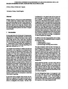
2. The Tensor Voting Framework 2.1. Tensor representation and voting The use of a voting process for feature inference from sparse and noisy data was formalized into a unified tensor framework by Medioni, Lee and Tang [8]. Input data is encoded as elementary tensors, then support information (including proximity and smoothness of continuity) is propagated by voting. Tensors that lie on smooth, salient features (such as curves or surfaces) strongly support each other and deform according to the prevailing orientation, producing generic tensors. Each such tensor encodes the local orientation of features (given by the tensor orientation), and their saliency (given by the tensor shape and size). Features can be then extracted by examining the tensors resulted after voting. r e1, λ1
r e3 , λ3
(a) generic tensor
r e2 , λ2
(b) stick tensor (surface element)
(c) plate tensor (curve element)
(d) ball tensor (point element)
Figure 1. Tensor representation in 3-D
In 3-D, a generic tensor can be visualized as an ellipsoid (Figure 1). It is described by a 3×3 eigensystem, where eigenvectors e1, e2, e3 give the ellipsoid orientation and eigenvalues λ1, λ2, λ3 give its shape and size. The tensor is represented as a matrix S = λ1 ⋅ e1e1T + λ 2 ⋅ e 2 e2T + λ3 ⋅ e3 e3T . There are three types of features in 3-D – surfaces, curves and points – that correspond to three elementary tensors, also shown in Figure 1. A surface element can be intuitively encoded as a stick tensor where one dimension dominates (along the surface normal), while the length of the stick represents the surface saliency (confidence in this knowledge). A curve element appears as a plate tensor where two dimensions co-dominate (in the plane of curve normals). A point element appears as a ball tensor where no dimension dominates, showing no preference for any particular orientation. Input tokens are encoded as such elementary tensors. A point element is encoded as a ball tensor, with e1, e2, e3 being any orthonormal basis, while λ1=λ2=λ3=1. A curve element is encoded as a plate tensor, with e1, e2 being normal to the curve, while λ1=λ2=1 and λ3=0. A surface element is encoded as a stick tensor, with e1 being normal to the surface, while λ1=1 and λ2=λ3=0. Tokens communicate through a voting process, where each token casts a vote at each token in its neighborhood. The size and shape of this neighborhood, and the vote strength and orientation are encapsulated in predefined voting fields (kernels), one for each feature type – there is a stick, a plate and a ball voting field in the 3-D case. At each receiving site, the collected votes are combined through simple tensor addition, producing generic tensors that reflect the saliency and orientation of the underlying smooth features. Local features can be extracted by examining the properties of a generic tensor, which can be decomposed in its stick, ball and plate components: S = (λ1 − λ 2 ) ⋅ e1 e1T + (λ 2 − λ 3 ) ⋅ ( e1 e1T + e2 e 2T ) + λ3 ⋅ (e e + e e + e e ) T 1 1
T 2 2
T 3 3
(1)
Each type of feature can be characterized as follows: • Surface: saliency is (λ1-λ2), normal orientation is e1 • Curve: saliency is (λ2-λ3), normal orientations are e1, e2 • Point: saliency is λ3, no preferred orientation
Therefore, the voting process infers surfaces, curves and junctions simultaneously, while also identifying outliers (tokens that receive little support). The method is noniterative, and does not depend on critical thresholds, the only free parameter being the scale factor σ which defines the voting fields. Vote generation. For simplicity of illustration, we describe the vote generation process in the 2-D case. Tensors in 2-D are ellipses (represented by 2x2 eigensystems) and the features are curves and points, corresponding to stick and ball tensors.
Q’
r N
r NP
Q
Q”
P (a) Vote orientation
(b) 2-D stick field
(c) 2-D ball field
Figure 2. Vote generation in 2-D r r Vote strength VS (d ) decays with distance | d | between voter and recipient, and with curvature ρ:
r2
|d | + ρ − r 2 VS ( d ) = e σ
2
(2)
Vote orientation corresponds to the smoothest local continuation from voter to recipient – see Figure 2. A tensor P where curve information is locally known r (illustrated by curve normal N P ) casts a vote at its neighbor Q. The vote orientation is chosen so that it ensures a smooth curve continuation through a circular arc from voter P to recipient Q. To propagate the curve r r normal N thus obtained, the vote Vstick (d ) sent from P to Q is encoded as a tensor according to: r r rr Vstick (d ) = VS (d ) ⋅ NN T
(3)
Figure 2(b) shows the 2-D stick field, with its color-coded strength. When the voter is a ball tensor, with no information known locally, the vote is generated by rotating a stick vote in the 2-D plane and integrating all contributions. The 2-D ball field is shown in Figure 2(c).
2.2. Extension to 4-D Table 1 shows all the geometric features that appear in a 4-D space and their representation as elementary 4-D Feature
λ1 λ2 λ3 λ4
e1 e2 e3 e4
Tensor
point
1 1 1 1
Any orth. basis
Ball
curve
1 1 1 0
n1 n2 n3 t
C-Plate
surface
1 1 0 0
n1 n2 t1 t2
S-Plate
volume
1 0 0 0
n t1 t2 t3
Stick
Table 1. Elementary tensors in 4-D Feature
Saliency
Normals
Tangents
point
λ4
none
none
curve
λ3 - λ4
e1 e2 e3
e4
surface
λ2 - λ3
e1 e2
e3 e4
volume
λ1 - λ2
e1
e2 e3 e4
Table 2. A generic tensor in 4-D
(a) Input images
(e) Layer boundaries
(b) Candidate matches
(c) Dense layers
(f) Epipolar lines
(d) Layer velocities
(g) 3-D structure and motion
Figure 3. BOOKS sequence
tensors, where n and t represent normal and tangent vectors, respectively. Note that a surface in the 4-D space can be characterized by two normal vectors, or by two tangent vectors. From a generic 4-D tensor that results after voting, the geometric features are extracted as shown in Table 2. The 4-D voting fields are obtained as follows. First the 4D stick field is generated in a similar manner to the 2-D stick field (see Figure 2). Then, the other three voting fields are built by integrating all the contributions obtained by rotating a 4-D stick field around appropriate axes. For example, the 4-D ball field is generated according to: 2π r r Vball (d ) = ∫ ∫∫ R Vstick (R −1d ) RT dθ xydθ xu dθ xv
(4)
0
where x, y, u, v are the 4-D coordinates axes and R is the rotation matrix with angles θxy, θxu, θxv. The data structure used to store the tensors is an approximate nearest neighbor (ANN) k-d tree [9]. The space complexity is O(n), where n is the input size (the total number of candidate tokens). The average time complexity of the voting process is O(µn) where µ is the average number of candidate tokens in the neighborhood. Therefore, in contrast to other voting techniques, such as the Hough Transform, both time and space complexities of the Tensor Voting methodology are independent of the dimensionality of the desired feature.
3. Grouping into Motion Layers We take as input two image frames that involve general motion – that is, both the camera and the objects in the scene may be moving. For illustration purposes, we give a description of our approach by using a specific example – the two images in Figure 3(a) are taken with a handheld moving camera, while the stack of books has also been moved between taking the two pictures.
Matching. For every pixel in the first image, the goal at this stage is to produce candidate matches in the second image. We use a normalized cross-correlation procedure, where all peaks of correlation are retained as candidates. Each candidate match is represented as a (x,y,vx,vy) point in the 4-D space of image coordinates and pixel velocities, with respect to the first image.
In order to increase the likelihood of including the correct match among the candidates, we repeat this process at multiple scales, by using different correlation window sizes. Small windows have the advantage of capturing fine detail, but produce considerable noise in areas lacking texture or having small repetitive patterns. Larger windows generate smoother matches, but their performance degrades in large areas along motion boundaries. We have experimented with a large range of window sizes, and found that best results are obtained by using only two or three different sizes, that should include at least a very small one. In practice we used three correlation windows, with 3x3, 5x5 and 7x7 sizes. The resulting candidates appear as a cloud of (x,y,vx,vy) points in the 4-D space. Figure 3(b) shows the candidate matches. In order to display 4-D data, the last component of each 4-D point has been dropped – the 3 dimensions shown are x and y (in the horizontal plane), and vx (the height). The motion layers can be already perceived as their tokens appear grouped in two layers surrounded by noisy matches. Extracting statistically salient structures from such noisy data is very difficult for most existing methods. Because our voting framework is robust to considerable amounts of noise, we can afford using the multiple window sizes in order to extract the motion layers. Selection. Since no information is initially known, each potential match is encoded as a 4-D ball tensor. Then each token casts votes by using the 4-D ball voting field. During voting there is strong support between tokens that lie on a smooth surface (layer) – therefore, for each pixel (x,y) we retain the candidate match with the highest surface saliency (λ2-λ3), and we reject the others as wrong
(a) Input images
(b) Candidate matches
(c) Velocities
(d) Dense layers
(e) 3-D structure
Figure 4. CYLINDERS sequence
(a) Input images
(e) Layer boundaries
(b) Candidate matches
(f) Epipolar lines
(c) Dense layers
(d) Layer velocities
(g) 3-D structure and motion
Figure 5. CAR sequence
matches. By voting we also estimate the normals to layers at each token as e1 and e2. Outlier rejection. In the selection step, we kept only the most salient candidate at each pixel. However, there are pixels where all candidates are wrong, such as in areas lacking texture. Therefore now we eliminate all tokens that have received very little support. Typically we reject all tokens with surface saliency less that 10% of the average saliency of the entire set. Densification. Since the previous step created holes (i.e., pixels where no velocity is available), we must infer them from the neighbors by using the smoothness constraint. For each pixel (x,y) without an assigned velocity we try to find the best (vx,vy) location at which to place a newly generated token. The candidates considered are all the discrete points (vx,vy) between the minimum and maximum velocities in the set, within a neighborhood of the (x,y) point. At each candidate position (x,y,vx,vy) we accumulate votes, according to the same Tensor Voting framework that we have used so far. After voting, the candidate token with maximal surface saliency (λ2-λ3) is retained, and its (vx,vy) coordinate represent the most likely velocity at (x,y). By following this procedure at every (x,y) image location we generate a dense velocity field. Note that in this process, along with velocities we simultaneously infer layer orientations. A 3-D view of the dense layers is shown in Figure 3(c). Segmentation. The next step is to group tokens into motion regions, by using again the smoothness constraint. We start from an arbitrary point in the image, assign a region label to it, and try to recursively propagate this
label to all its image neighbors. In order to decide whether the label must be propagated, we use the smoothness of both velocity and layer orientation as a grouping criterion. Figure 3(d) illustrates the recovered vx velocities within layers (dark corresponds to low velocity). Boundary inference. The extracted layers may still be over or under-extended along the true object boundaries, typically due to occlusion. The boundaries of the extracted layers give us a good estimate for the position and overall orientation of the true boundaries. We combine this knowledge with monocular cues (intensity edges) from the original images in order to build a boundary saliency map within the uncertainty zone along the layers margins. At each location in this area, a 2-D stick tensor is generated, having an orientation normal to the image gradient, and a saliency proportional to the gradient magnitude.
The smoothness and continuity of the boundary is then enforced through a 2-D voting process, and the true boundary is extracted as the most salient curve within the saliency map. Finally, pixels from the uncertainty zone are reassigned to regions according to the new boundaries, and their velocities are recomputed. Figure 3(e) shows the refined motion boundaries, that indeed correspond to the actual objects.
4. Three-Dimensional Interpretation So far we have not made any assumption regarding the 3D motion, and the only constraint used has been the smoothness of image motion. The observed image motion could have been produced by the 3-D motion of objects in
(a) Input images
(e) Layer boundaries
(b) Candidate matches
(c) Dense layers
(d) Layer velocities
(g) 3-D structure and motion
(f) Epipolar lines
Figure 6. CANDY BOX sequence
(a) Input images
(b) Candidate matches (vx)
(c) Velocities
(d) Dense layers (vx)
(e) Dense layers (vy)
Figure 7. FLAG sequence
the scene, or the camera motion, or both. Furthermore, some of the objects may suffer non-rigid motion. For classification we used an algorithm introduced by McReynolds and Lowe [10], that verifies the potential rigidity of a set of minimum six point correspondences from two views under perspective projection. The rigidity test is performed on a subset of matches within each object, to identify potentially rigid objects, and also across objects, to merge those that move rigidly together but have distinct image motions due to depth discontinuities. It is also worth mentioning that the rigidity test is actually able to only guarantee the non-rigidity of a given configuration. Indeed, if the rigidity test fails, it means that the image motion is not compatible to a rigid 3-D motion, and therefore the configuration must be non-rigid. If the test succeeds, it only asserts that a possible rigid 3D motion exists, that is compatible to the given image motion. However, this computational approach corresponds to the way human vision operates – as shown in [11], human perception solves this inherent ambiguity by always choosing a rigid interpretation when possible. The remaining task at this stage is to determine the 3-D object (or camera) motion, and the scene structure. Since wrong matches have been eliminated, and correct matches are already grouped according to the rigidly moving objects in the scene, standard methods for reconstruction can be reliably applied. For increased robustness, we chose to use RANSAC [3] to recover the epipolar geometry for each rigid object, followed by an estimation of camera motion and projective scene structure.
Multiple rigid motions. This case is illustrated by the BOOKS example in Figure 3, where two sets of matches have been detected, corresponding to the two distinct objects – the stack of books and the background. The rigidity test shows that, while each object moves rigidly, they cannot be merged into a single rigid structure. The two sets of recovered epipolar lines are illustrated in Figure 3(f), while the 3-D scene structure and motion are shown in Figure 3(g).
The CYLINDERS example, shown in Figure 4, is adapted from Ullman [11], and consists of two images of random points in a sparse configuration, taken from the surfaces of two transparent co-axial cylinders, rotating in opposite directions. This extremely difficult example clearly illustrates the power of our approach, which is able to determine accurate point correspondences and scene structure – even from a sparse input, based on motion cues only (without any monocular cues), and for transparent motion. In the CAR example, shown in Figure 5, the sign and the background correspond to a rigid configuration and can be merged, while the car exhibits an independent motion. Single rigid motion. This is the stereo case, illustrated by the CANDY BOX example in Figure 6, where the scene is static and the camera is moving. Due to the depth disparity between the box and the background, they exhibit different image motions, and thus they have been segmented as two separate objects. However, the rigidity test shows that the two objects form a rigid configuration, and therefore the epipolar geometry estimation and scene
(a) An input image
(b) Ground truth disparity map
Methods
Error Rate
Tensor Voting
15.4%
Sum of Squared Differences
26.5%
Dynamic Programming
30.1%
Graph Cuts
29.3%
(c) Tensor Voting disparity map
Figure 8. TEDDY sequence
Table 3. TEDDY sequence – results
reconstruction are performed on the entire set of matches. Along with the 3-D structure, Figure 6(g) also shows the two recovered camera positions.
possibility of using an adaptive scale of analysis in the voting process.
Non-rigid motion. The FLAG example, shown in Figure 7, is a synthetic sequence where sparse random dots from the surface of a waving flag are displayed in two frames. The configuration is recognized as non-rigid, and therefore no reconstruction is attempted. However, since the image motion is smooth, our framework is still able to determine correct correspondences, extract motion layers, segment non-rigid objects, and label them as such.
6. Acknowledgements
We also analyzed a standard sequence (the TEDDY example – Figure 8) with ground truth available, to provide a quantitative estimate for the performance of our approach, as compared to other methods. As shown in Table 3 (partially reproduced from [12]), our voting-based approach has the smallest error rate (percentage of pixels with a disparity error greater than 1), among the techniques mentioned.
5. Conclusions We have presented a novel approach that decouples grouping and interpretation of visual motion, allowing for explicit and separate handling of matching, outlier rejection, grouping, and recovery of camera and scene structure. The advantage of the proposed framework over existing methods is its ability to handle data sets that simultaneously contain large amounts of outlier noise and multiple independently moving objects. Our methodology for extracting motion layers is based on a layered 4-D representation of data, and a voting scheme for token communication. It allows for structure inference without using any prior knowledge of the motion model, based on the smoothness of image motion only, while consistently handling both smooth moving regions and motion discontinuities. The method is also computationally robust, being non-iterative, and does not depend on critical thresholds, the only free parameter being the scale of analysis. We plan to extend our approach by incorporating information from multiple frames, and to study the
This research has been funded in part by the Integrated Media Systems Center, an NSF Engineering Research Center, Cooperative Agreement No. EEC-9529152, and by NSF Grant 9811883.
References [1] H. C. Longuet-Higgins, A computer algorithm for reconstructing a scene from two projections, Nature, 293, 1981, 133-135. [2] R. I. Hartley, In defense of the 8-point algorithm, Trans. PAMI, 19(6), 1997, 580-593. [3] P. Torr, D. Murray, A review of robust methods to estimate the fundamental matrix, IJCV, 1997. [4] Z. Zhang, Determining the epipolar geometry and its uncertainty: a review, IJCV, 27(2), 1998, 161-195. [5] M. Nicolescu, G. Medioni, 4-D voting for matching, densification and segmentation into motion layers, ICPR, 2002. [6] A. Adam, E. Rivlin, L. Shimshoni, Ror: rejection of outliers by rotations, Trans. PAMI, 23(1), 2001, 7884. [7] P. Pritchett, A. Zisserman, Wide baseline stereo matching, ICCV, 1998, 754-760. [8] G. Medioni, M-S. Lee, C-K. Tang, A computational framework for segmentation and grouping (Elsevier Science, 2000). [9] S. Arya, D. Mount, N. Netanyahu, R Silverman, A. Wu, An optimal algorithm for approximate nearest neighbor searching in fixed dimensions, Journal of the ACM, 45(6), 1998, 891-923. [10] D. McReynolds, D. Lowe, Rigidity checking of 3D point correspondences under perspective projection, Trans. PAMI, 18(12), 1996, 1174-1185. [11] S. Ullman, The interpretation of visual motion (MIT Press, 1979). [12] D. Scharstein, R. Szeliski, High-accuracy stereo depth maps using structured light, CVPR, 2003, 195202.