Robustness of Real and Virtual Queue based Active Queue Management Schemes∗ Ashvin Lakshmikantha, C. L. Beck and R. Srikant Department of General Engineering University of Illinois
[email protected],
[email protected],
[email protected] November 12, 2002
Abstract In this paper, we compare the performances of the real and virtual queue based marking schemes used at the routers in the Internet. Using simple fluid flow models, we show via analysis and simulations that a Virtual Queue (VQ) based marking scheme is superior to a Real Queue (RQ) based marking scheme in terms of robustness to disturbances and the ability to maintain low queueing delays. Our analytical results are applicable to the combinations of proportionally-fair and TCP-type congestion controllers at the sources, and REM and Proportional Control (PC) at the routers. The behavior of RED and PI controllers at the routers are studied via simulations.
1 Introduction In recent years, there has been a significant interest in the design of a low-loss, low-delay Internet [7, 8, 10, 12, 13]. The primary enabling technology for this is the possible introduction of Early Congestion Notification (ECN) capability at the routers. Unlike the traditional congestion notification mechanism whereby routers drop packets to signal congestion, with ECN, routers have the capability to mark a packet to indicate congestion. Marking refers to the process of flipping a bit in the packet header from a zero to a one when the router detects incipient congestion. Each receiver echoes the marks to its source and the source is expected to respond to each mark by reducing its transmission rate. In this paper, we focus on the mechanism by which marking is performed at the routers. Specifically, we compare schemes where a router marks packets based on its queue length to schemes where the router marks packets based on the queue length of a virtual queue (VQ) [4]. A virtual queue is a fictitious queue maintained at each link whose capacity is less than the actual capacity of the link. The idea behind maintaining a ∗
Research supported by AFOSR grant F49620-01-1-0365 and DARPA grant F30602-00-2-0542
1
virtual queue is that it provides early warning about congestion since the virtual queue’s capacity is smaller than the capacity of the real queue. We consider the following congestion control mechanisms at the router: a proportionally fair congestion controller (PFC) [6] and a minimum potential delay controller [14]. Due to its similarity to the TCP congestion avoidance algorithm [9], we refer to the minimum potential delay controller as a TCP-type congestion controller. We consider the following Active Queue Management (AQM) schemes at the router: RED (random early detection) [3], REM (random early marking) [1], PC (proportional control) [5] and PI control [5]. We compare implementations of each of these AQM schemes on the real queue with implementations on a virtual queue. We show through a combination of analysis and simulation that, by using a virtual queue and reducing the link utilization from 100% to slightly less than 100% (say, 95%), we can acheive a significant improvement in the performance of the network. We consider two criteria for assessing the performance of the network: • Queueing delay: We want the queueing delay to be a small fraction of the propagation delay in the network. • Robustness: In most models of congestion control, it is typically assumed that flows are long-lived and thus, steady-state stability analysis is reasonable. However, in a real network, there are many sources of disturbances such as short-lived flows (popularly known as web mice) and sources that do not respond to congestion notification such as real-time flows. In this paper, we evaluate the robustness of our system with respect to these unmodelled disturbances. Specifically, we evaluate the intensity of disturbance traffic that the system can tolerate while maintaining small queue lengths. We first consider the case of PFC with REM at the router. We present necessary conditions that the controller and the REM parameters should satisfy to ensure local stability of this system with delayed feedback. Using this, we show that it is not possible to have very low queueing delays in the presence of disturbances. Further, we will show that if REM is implemented in a virtual queue, both stability and small queueing delays can be achieved for any value of link utilization smaller than one. We then show that the same phenomenon occurs for the following combinations of source controllers and AQM schemes: PFC and Proportional Control (PC), TCP and REM, and TCP and PC. Proportional Control at the router is an AQM scheme that captures the behavior of RED when queue length averaging is not performed. Thus, by proportional control we mean that the instantaneous queue length is used along with the RED-marking profile. Additional congestion control/AQM scheme combinations are studied via simulations with the following results. 1. PFC/RED, TCP/RED: The same results that were analytically established for the PFC/PC and TCP/PC combinations seem to hold for this case. 2. PFC/PI, TCP/PI : In all of the previous cases, the RQ-based controllers perform worse than the VQ-based controllers even in the presence of constant disturbances. Interestingly, this is no longer the case with the
2
PI controller. In fact all our simulations seem to indicate that the PI controller is robust to deterministic disturbances with or without a VQ. However, these results change dramatically in the presence of random disturbances, which are more realistic in modeling short flows in the Internet. As the fraction of the total capacity occupied by these short flows increases, the queue length in the case of RQ-based PI increases, but the VQ-based PI control continues to maintain a small queue length. The main contribution of this paper is the demonstration of the fact that marking based on a VQ is more robust in the sense that the system is locally stable and is able to maintain small queue lengths even in the presence of disturbances. Further, based on our analytical and simulation studies, we can conclude that when a VQ-based scheme is used, the choice of the specific AQM scheme seems to be less important. However, among RQ-based schemes, PI control seems to perform better than the other schemes that we have considered. The intuitive reason for the robustness of a VQ-based AQM scheme is as follows: in a VQ-based scheme, the queue length is guaranteed to be small since the arrival rate is less than the link capacity. Thus, the system parameters have to be designed only to maintain stability in the presence of disturbances. On the other hand, with RQ-based AQM schemes, one has further to design the system to maintain small queue lengths. Thus, in a sense, VQ-based schemes have an additional degree of freedom which allows us to choose the system parameters to stabilize the system even in the presence of unknown disturbances. We note that we do not consider adapting the virtual capacity to changing network traffic conditions. Typically, this is performed on a time scale that is slower than the dynamics of the congestion controllers [12, 10, 11], whereas the analysis in this paper is appropriate for models at the congestion-control time scale. The rest of the paper is organized as follows. In Section 2, we present the models for the various congestion controllers and AQM schemes used in this paper. In Section 3, we present the main analytical results. Section 4 contains simulation results that strengthen the observations made in Section 3 and provide further insight into those combinations of controllers/AQM schemes that are not addressed in Section 3. Concluding remarks are provided in Section 5.
2 Models of Congestion Controllers and AQM Schemes We consider a deterministic fluid model of a single congestion-controlled source1 accessing a single link. Suppose that the transmission rate of the user at time t is denoted by x(t), the link capacity is denoted by C, and queue length is denoted by q. In addition to the congestion controlled source, we also assume that a fraction of the link’s capacity is occupied by short flows or unresponsive flows. Let δ denote the fraction of the link’s capacity that is used by these disturbance processes. Then the evolution of the queue is governed by the equation q˙ = x(t) + δC − C, = (x(t) + δC − C)+ , 1
q>0
(1)
q = 0.
The analysis can be easily extended to the case of multiple sources with equal delay by appropriately rescaling the system parameters.
3
Similarly if a virtual queue is maintained at the router, then the evolution of the virtual queue length is given by ˜ q˙v = x(t) + δC − C, q>0 ³ ´+ q = 0. = x(t) + δC − C˜ ,
(2)
where C˜ < C. Denoting the desired utilization by γ, i.e., C˜ = γC, we can write q˙v = x(t) + δC − γC, = (x(t) + δC − γC)+ ,
q>0
(3)
q = 0.
Congestion Control Schemes We consider two types of dynamics for the source rate x(t) : 1. PFC (Proportionally-Fair Controller): Let P (q) denote the probability that a packet is marked at the link when the queue length is q. The PFC is then given by x˙ = κ [∆ − x(t − τ (t))P (q(t − τ (t)))] ,
(4)
where the right-hand side of the above equation has to be appropriately modified to account for the fact that the source rate is always non-negative. Here κ and ∆ are controller parameters, and τ denotes the feedback delay (also known as round-trip time or RTT) in the network. The RTT is the sum of two components: the propagation delay, which we denote by τpr , and the queueing delay
q(t) C .
We also note that (4) should be
modified by replacing P (q) with P (qv ) when marking is done based on the virtual queue length. 2. TCP-type congestion controller: The congestion avoidance phase of the TCP-type congestion controller can be modeled as x˙ =
1 − αx(t)x(t − τ (t))P (q(t − τ (t))) τ2
where α = 32 , and P (q), q and τ are defined as before. The value of and [9] where a value of ln(2) (which is close to
2 3)
2 3
(5)
for α is justified by the analysis in [15]
is suggested for β . For our analysis, we will consider the
following general form of the controller: x˙ = κ [∆ − βx(t)x(t − τ (t))P (q(t − τ (t)))] . Note that through appropriate choice of κ, ∆ and β, (6) can be put in the form (5).
AQM schemes We consider the following AQM schemes.
4
(6)
1. REM : The marking probability function used by REM is given by P (q) = 1 − e−θq ,
(7)
where q is the instantaneous queue length at the buffer (which may be real or virtual depending on the policy at the router), and θ is a parameter that determines the responsiveness of the router to incipient congestion. Higher values of θ lead to higher marking probability, which means the router is more aggressive in responding to congestion. 2. RED: The RED algorithm maintains an average queue length which we denote by qavg . The average queue length at any time t is computed as a weighted sum of the current queue length and the previous value of the average queue length. The marking probability is chosen as a function of the average queue length as follows: • if qavg < qmin , then P (q) = 0. • if qmin < qavg < qmax , then P (q) = Kp (qavg − qmin ) • if qavg > qmax P (q) = 1.0, where qmax and qmin are user-defined thresholds and Kp is a constant. As in [5], we approximate this behavior by the following differential equation P˙ = K(Kp q(t) − P (q(t))),
(8)
where K is a function of the averaging parameter used in computing qavg . 3. PI: A PI controller is of the following form: P˙ = Kpi
µ
q˙ + q − qref η
,
(9)
where Kpi and η are controller gains which may be chosen to control the system behavior, and qref is the desired queue length. 4. PC : The PC (Proportional Control) algorithm marks packets with a probability that is directly proportional to the instantaneous queue length, that is, P (q) = Kp q,
(10)
where Kp is a proportionality constant.
3 Analytical Results We begin by stating a basic theorem regarding the stability of delay differential equations. This result is used extensively throughout the paper and provides a means of assessing the maximum delay interval over which a delay 5
differential equation is stable. In particular, we present a version of the result given in [2] for delay differential equations of the following form:
x˙ = Ax(t) + A1 x(t − τ ),
(11)
where A,Ai ∈ ℜn×n and τ is the delay parameter. In the theorem, the following notation is used. We define the generalized eigenvalue λ(A, B) of two n × n matrices A and B as any solution λ to the equation det(A − λB) = 0. For convenience, we denote the n generalized eigenvalues by λ1 (A, B) through λn (A, B). Further, let ρ(A, B) := min{|λ| : det(A − λB) = 0}. Theorem 1 Let rank(A1 ) = m. Suppose the system (11) is stable for some τ ∗ ∈ [0, ∞). Define i min1≤k≤n αki if λi (jω i I − A, A1 e−jτ ωki ) = e−jαik for some ω i ∈ (0, ∞) k k ωk τi+ = i ∞ if ρ(jωki I − A, A1 e−jτ ωk ) > 1 for all ωki ∈ (0, ∞) Further, define
τ + = min τi+ 1≤i≤m
Then the following statements are true. 1. The system is stable for any τ ∈ [τ ∗ , τ ∗ + τ + ). 2. The system becomes unstable at τ = τ ∗ + τ + . ⋄
3.1
PFC and REM based on RQ
We first study a proportionally-fair controller with REM at the router and no uncontrolled disturbances at the link, i.e., we let δ = 0. The system of delay differential equations given in (4), (7) and (1) is nonlinear. To apply Theorem 1, we linearize (1) and (4) about the equilibrium point. Thus, we study only the local stability of (1) and (4). The equilibrium point of (1) and (4), with REM used at the router, is given by xe = C µ ¶ 1 C qe = log . θ C −∆
6
(12)
Suppose we perturb the equilibrium values of the source rate and queue length by y(t) and r(t), respectively, i.e., x(t) = xe + y(t),
(13)
q(t) = qe + r(t). Linearizing around (xe , qe ) yields the following linear delay differential equation for (y(t), r(t)) : X˙ = AX + A1 X(t − τ ) where
A=
and
0 0 1 0
X=
y
r
, A1 =
(14)
,
′
−κPe −κxe Pe
τ = τpr +
0
0
,
qe . C
In the above differential equation, Pe denotes the equilibrium value for the marking probability (and is equal to
∆ C ),
′
and Pe denotes the first derivative of P (q) evaluated at qe . We then have the following stability result as a direct consequence of Theorem 1. Corollary 2 The system defined by (14) is stable for all values of τ < τ ∗ where τ ∗ is given by µ ¶ 1 Pe ω ∗ −1 τ = tan ω CPe′
(15)
and ω is a positive solution of the equation ′
ω 4 − κ2 Pe2 ω 2 − κ2 C 2 (Pe )2 = 0.
(16)
Proof. First note that the system is stable when τ = 0, then apply Theorem 1. The above theorem provides a condition to test for the stability of the system. The following lemma proves that it is always possible to choose parameters so that the linear system is stable. Lemma 3 Given τpr , ∆ and C it is always possible to choose θ and κ such that the system is stable.
7
Proof. The condition for stability from Corollary 1 is ¶ ¶ µ µ 1 1 Pe ω ∆ω −1 −1 = tan τ < tan , ω ω C(C − ∆)θ CPe′
(17)
where τ = τpr + Substituting for qe we have 1 τ = τpr + log Cθ
qe . C
µ
C C −∆
.
Therefore (17) can be rewritten as τpr
1 < tan−1 ω
µ
Pe ω CPe′
1 − log θC
µ
C C −∆
.
(18)
From (16), when κ → 0, ω → 0. Hence 1 lim tan−1 κ→0 ω
µ
∆ω C(C − ∆)θ
=
∆ . C(C − ∆)θ
Therefore given an ǫ > 0, there exists κ such that µ ¶ 1 ∆ω ∆ −1 tan − ǫ. > ω C(C − ∆)θ C(C − ∆)θ
(19)
From (18) and (19) we can write ¶ µ µ ¶ ¶ µ C ∆ ∆ω C 1 1 1 −1 − Cθǫ − log( ) < tan log − . τpr < Cθ (C − ∆) C −∆ ω C(C − ∆)θ θC C −∆ Using the fact that x − log(1 + x) > 0 for all x > 0, it is now easy to see that, by choosing κ and θ sufficiently small, the stability condition can be satisfied. Recall that the equilibrium value of the queueing delay is given by
qe C.
Our goal is to ensure system stability while
keeping the queueing delay small. The following theorem shows that this is possible only if the equilibrium marking probability is large (close to 1). Theorem 4 Suppose that the system parameters are chosen such that the linearized form of the system given by (4), (7) and (1) is stable and
qe C
< ǫτpr for some ǫ > 0. Then, Pe must satisfy the following inequality: µ ¶ 1 − Pe Pe ǫ > log 1 + . 1+ǫ Pe 1 − Pe
Thus, ǫ → 0 implies Pe → 1. In other words, if we require the queueing delay to be a small fraction of the propagation delay and require that the system is stable, then the equilibrium marking probability must be very high.
8
Proof. From Corollary 2, for stability, we need 1 τ < tan−1 ω
µ
Pe ω CPe′
,
where ω > 0 is a solution of the equation ′
ω 4 − κ2 Pe2 ω 2 − κ2 C 2 (Pe )2 = 0. Since tan−1 (x) < x for x > 0, a necessary condition for stability is given by Pe ∆ . = C(C − ∆)θ CPe′
τ
τpr + τq
µ
1 − Pe Pe
µ log 1 +
Pe 1 − Pe
.
(21)
If we require that qe < ǫ, Cτpr then (21) can be written as ǫ > ǫ+1 Now it is clear that as ǫ → 0, Pe → 1.
µ
1 − Pe Pe
µ
Pe log 1 + 1 − Pe
.
As an example, suppose that the equilibrium queueing delay is required to be less than 10% of the propagation delay. Then, it is easy to show that Pe must be greater than 0.975. We now consider the effect of disturbances, which may be represented by the system (4) and (1) with the parameter δ ∈ (0, 1). Linearizing the system about the equilibrium gives X˙ = AX + A1 X(t − τ ) where
X=
y r
,
A=
0 0 1 0
,
and A1 =
(22)
′
−κPe (δ) −κxe (δ)Pe (δ) 0
0
.
We assume that δ is a constant whose value is not known apriori. Thus, we have a linear system whose parameters are unknown. We would like to ensure stability and also maintain low queueing delays in the presence of disturbances. 9
In other words, we are interested in finding the range of δ for which the system is stable when the original system is designed assuming δ = 0. The following lemma states that designing the system for low queueing delays results in poor disturbance rejection properties, i.e., stability is maintained only when δ is very small. Lemma 5 Suppose that the parameters of the linearized form of the system (1) and (4) are designed to maintain stability and low queueing delays (i.e.
qe C
< ǫτq , where ǫ is small) in the absence of disturbances. Then, as ǫ → 0,
to ensure stability, δ must decrease to 0. Proof. Let Penom denote the design value of the equilibrium marking probability, i.e., when δ = 0. In other words, Penom =
∆ . C
Let the actual disturbance level at the router be denoted by δ. The equilibrium throughput is then given by xe = C(1 − δ). Let the actual equilibrium marking probability be denoted by Pe (δ). Since Pe (δ) < 1, we have ∆ < 1, (1 − δ)C or equivalently δ < 1 − Penom . Clearly as Penom → 1, δ → 0, and the result follows from Theorem 4. In other words, if the system is designed to maintain both stability and low queueing delays, then only low levels of disturbances can be handled at the router. In the next theorem, we show that designing the system for a disturbance level of δmax would result in instability when the system experiences a lower level of disturbance. Theorem 6 Suppose that the parameters of the linearized form of system (1) and (4) are designed so that the system qe maintains stability and low queueing delays ( Cτ < ǫ) when the disturbance level is δmax . Then given any δc < δmax
there exists ǫc > 0 such that for all ǫ < ǫc , the linear stability condition is violated for all δ ∈ [0, δc ]. In other words, a controller design based on the linear stability criterion cannot maintain small queueing delays if the disturbance is unknown. Proof. The equilibrium marking probability when the disturbance is δmax is given by Pe (δmax ) =
∆ . C(1 − δmax )
From the conditions for stability, we have ¶ µ ∆ ∆ω 1 −1 < . τpr ≤ τ < tan ω C(1 − δmax )(C(1 − δmax ) − ∆)θ C(1 − δmax )(C(1 − δmax ) − ∆)θ 10
From Lemma 3, it is always possible to choose θ and κ such that the system is stable. Hence, we can write τpr =
ν∆ , C(1 − δmax )(C(1 − δmax ) − ∆)θ
(23)
where ν ∈ (0, 1) is some fixed constant. Now, suppose that the system experiences a disturbance of δ < δmax , the system must then satisfy τ
0 such that for all ǫ < ǫc and δ ∈ [0, δc ] the system is unstable.
From the above analysis we can conclude the following. • To achieve low queueing delays with a RQ-based REM, one has to have very high equilibrium marking probability (Pe ). Since Pe is simply ∆/C, this implies that ∆ has to be large. In other words, the QoS (quality of service) requirement that the queueing delay should be small constrains the possible values for ∆. • Since one of the system parameters, ∆, is constrained due to our QoS requirement, it limits our ability to choose the system parameters for the purpose of disturbance rejection. As a result, the system has poor disturbance rejection properties. • In other words, it is not possible to maintain low queueing delays and reject disturbances unless the disturbance level is known a priori.
3.2
PFC and REM based on VQ
We first consider the VQ-based marking system represented by (3) and (4) with δ = 0. Linearizing this system about the equilibrium point gives the system represented by (14), but with a different set of equilibrium values given by xe = γd C 11
Pe =
∆ , γd C
where γd denotes the design value of γ. The stability conditions for the VQ-based AQM scheme, which are a direct consequence of Theorem 1, are stated in the following corollary. Corollary 7 The system is stable for all values of τ < τ ∗ where τ ∗ is given by µ ¶ 1 Pe ω ∗ −1 τ = tan ω γd CPe′ and ω is a positive solution of the equation ′
ω 4 − κ2 Pe2 ω 2 − κ2 C 2 (Pe )2 = 0. ⋄ Now, as in Lemma 3, it can readily be shown that in the case of a VQ-based controller, given τ, ∆, γd and C, it is always possible to choose θ and κ such that the system is stable. For a VQ-based controller, the equilibrium value of the real queue is zero since the equilibrium arrival rate is less than the link capacity. Hence the queueing delay is always zero. Thus, unlike the RQ case, an upper bound on the queueing delay does not impose any restriction on the system parameters. As we will see, this allows us to achieve better disturbance rejection properties in a VQ-based system. We now consider the effect of disturbances in VQ-based systems. Specifically, consider the system defined by (3) and (4) with δ 6= 0. The rate at which the queue length grows is given by q˙ = x(t) − γd C + δC. The equilibrium rate at which the user can send data is given by xe = (γd − δ)C. Now, since Pe (δ) < 1, we have ∆ < 1, (γd − δ)C or equivalently δ < γd −
∆ . C
The main theorem of this section states that, given an upper bound on the disturbance level, it is possible to ensure that the system is stable for all levels of disturbance less than this upper bound. We first state and prove the following lemma regarding the uniform convergence of a sequence of functions, which is used in the main theorem.
12
Replacing κ by n1 , where n ∈ N, we consider the following sequence of real-valued functions: ! Ã 1 ) ∆ω(γ, 1 n fn (γ) = . tan−1 γC(γC − ∆)θ ω(γ, n1 ) Given δmax < γd −
∆ C,
(25)
an upper bound on the disturbance, the sequence of functions {fn } is defined in the domain
[γd − δmax , γd ]. In this domain, the sequence of functions converge pointwise to ∆ . γC(γC − ∆)θ
f (γ) = ′
Let fn denote the first derivative of fn w.r.t γ. Recall that ω is the positive root of the equation given in Corollary 7, that is,
µ ¶2 µ ¶ µ ¶2 1 ∆ 2 2 1 ω − (θ(γC − ∆))2 = 0, n γC n
ω4 −
Note that as n → ∞, κ → 0 and ω(γ, n1 ) → 0.
Lemma 8 The sequence of functions {fn } converges uniformly to f in the domain D := [γd − δmax , γd ]. ′
Proof. We first prove that the sequence of functions {fn } and {fn } are uniformly bounded. Note that for any n, the function fn (γ) has no singularities in D. Further fn (γ) is clearly bounded above by f (γ) for all n ∈ N, and f (γ) has no singularities in D. Hence fn is uniformly bounded. Differentiating fn w.r.t γ gives ∂ω(γ, n1 ) dfn 1 fn (γ) = = F1 − F2 , dγ ∂γ ω(γ, n1 ) ′
where
F1 =
−1 tan−1 ω(γ, n1 )
F2 =
and
Ã
1 n)
∆ω(γ, γC(γC − ∆)θ
1 1+
³
1 ∆ω(γ, n )
γC(γC−∆)θ
´2
∂ω(γ, 1 1 ∂γ ω(γ, n )
1 n)
! µ
+
g4 =
∆2 γ3C2 ∆4 γ4C4
g2 = g5 =
1+
− n1 g1 + =
∆4 γ5C4 4θ2 (γC
1 ∆ω(γ, n )
γC(γC−∆)θ
( n1 )g6
∆ ´2 γC(γC − ∆)θ ,
1 C + 2 γ (γC − ∆) γ(γC − ∆)2
Here, gi denote continuous bounded functions of γ given by g1 =
1 ³
(26)
∆ , Cθ
(27)
(28)
−( 1 )2 g2 +g3 q n 1 2 ) g4 +g5 (n
q . + ( n1 )2 g4 + g5 g3 = 2θ2 (γC − ∆)C
− ∆)2 g6 =
∆2 . γ2C2
′
It is straightforward to show that the sequence {fn } is also uniformly bounded. This implies that the family of functions {fn } is equicontinuous. A direct application of the Arzela-Ascoli theorem (see, for example, [16]) gives the result.
13
Theorem 9 Consider the linearized form of the system defined by (3) and (4) with δ 6= 0. Let γd denote the design value of γ. Given an upper bound δmax < γd −
∆ C
on the disturbance level, there exist κ and θ such that the system
is stable for any δ < δmax . Proof. Fix θ > 0 and consider the sequence of functions defined in (25). By Lemma 8, we know that given any ǫ > 0 there exists an N such that, for all n > N , f − fn < ǫ for all γ ∈ [γd − δmax , γd ]. Letting κ =
1 n
and defining fκ accordingly, we can equivalently state that given any
ǫ > 0 there exists κ such that f − fκ < ǫ for all γ ∈ [γd − δmax , γd ]. The following inequality clearly holds:
1
1+
Thus there exists a κ > 0 such that
or equivalently,
1+
³
∆ω(γ,κ) γC(γC−∆)θ
1 ³
∆ω(γ,κ) γC(γC−∆)θ
´2
´2
∆ < f. γC(γC − ∆)θ
∆ − fκ < ǫ, γC(γC − ∆)θ
F1 < ǫ, where F1 is defined in (27). Therefore, there exists κ > 0 such that 1 ∂ω(γ, κ) 1 ∂ω(γ, κ) dfκ = F1 − F2 < ǫ − F2 dγ ω(γ, κ) ∂γ ω(γ, κ) ∂γ for all γ ∈ [γd − δmax , γd ], with F2 as defined in (28). Note that ǫ can be made arbitrarily small. Further, as κ → 0, F2 > µ for some µ > 0. Hence it follows that there exists a κ > 0 such that dfκ 0 such that fκ is a decreasing function of γ, implying that if δ < δmax , then 1 τ< tan−1 ω(γd , κ)
µ
∆ω(γd , κ) γd C(γd C − ∆)θ
1 tan−1 < ω((γd − δ), κ)
µ
∆ω((γd − δ), κ) (γd − δ)C((γd − δ)C − ∆)θ
.
Thus the system is stable for all δ < δmax . Remark 1 The previous theorem states that the system is stable for all δ < γ −
∆ C.
Thus, by choosing ∆ small, we ⋄
can reject large levels of disturbances.
14
3.3
Analysis of a TCP-REM based on RQ and VQ
TCP-type congestion controllers can be analyzed in a manner similar to the analysis in the previous two subsections. The system is now defined by (1) and (6). The equilibrium point is given by xe = C and qe =
βC 2 1 log( ), θ βC 2 − ∆
when RQ-based marking is used. In the case of VQ-based schemes, the equilibrium points change appropriately. The following analysis is done considering a RQ-based REM at the router. Linearizing this system gives X˙ = AX + A1 X(t − τ ) where
and
X=
y r
, A =
−κPe xe 0 1
0
, A1 =
τ = τpr +
(29)
′
−κPe xe −κx2e Pe 0
0
qe , C
′
where Pe is the equilibrium marking probability and Pe is the first derivative of Pe evaluated at qe . Again, as a direct consequence of Theorem 1 we can state the following. Corollary 10 The system is stable for all τ < τ ∗ where τ∗ =
Pe ω 2 tan−1 ( ) ω CPe′
and ω=
p κPe ′ x2e .
⋄
We now derive stability conditions under the constraint that the queueing delays remain small. Theorem 11 Suppose that the system parameters are chosen such that the linearized form of the system given in (6), (7) and (1) is stable and
qe C
< ǫτpr for some ǫ > 0. Then Pe must satisfy the following inequality: µ ¶ ǫ 1 − Pe Pe > log 1 + . 1+ǫ 2Pe 1 − Pe
Thus, ǫ → 0 implies Pe → 1. In other words, if we require the queueing delay to be a small fraction of the propagation delay and we require that the system is stable, then the equilibrium marking probability must be very high.
15
Proof. The proof of this theorem is similar to the proof of Theorem 4. This result implies that to achieve a low queueing delay one must have a high equilibrium marking probability. A disturbance rejection analysis similar to that for PFC and RQ-based REM shows that it is not possible to simultaneously ensure stability, disturbance rejection and small queueing delays. Similar to the analysis in Section 3.2, it can be shown that, in the case of a TCP-type congestion controller and VQ-based REM, it is possible to maintain both stability and low queueing delays in presence of large levels of disturbance.
3.4
Analysis of a PFC-PC and TCP-PC based on RQ and VQ
Consider a PFC at the source and RQ-based PC at the router. It follows from Theorem 1 that the system is stable if µ ¶ 1 Pe ω −1 τ < tan . ω Pe′ C As tan−1 (x) < x, a necessary condition for stability would be, τ
. τ 2 Further analysis similar to Section 3.2 reveals that it is possible to reject large disturbance levels with a VQ-based PC while maintaining stability and low queueing delays.
16
Queueing Delay/Propagation Delay
3.5
3
2.5
2
1.5
1
0.5
0
0
5
10
15
20
25
30
35
40
45
50
Time
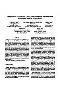
Figure 1: Evolution of the Queueing delay with PFC at the source, RQ-based REM at the router and a constant disturbance of 3.1% of link capacity
4 Simulations In this section, we demonstrate the robustness of VQ-based congestion controllers via simulations. We study REM, PI and RED marking schemes at the router, along with PFC and TCP-type congestion controllers at the source. For all virtual queues, the target utilization γd is set to 0.95. The capacity C is chosen to be 10000 packets/sec. (The bandwidth associated with this is approximately equal to the bandwidth of 100 Mbps link, assuming that each packet is 1000 bytes long). The number of users is 1000. The roundtrip propagation delay for all users is taken to be 40 msec. Although the analysis in the earlier sections was carried out treating the disturbance as an unknown constant, in these simulations random flows are taken into account. Whenever the system is simulated in the presence of random flows, we take these random flows to be i.i.d. Bernoulli random variables with the total mean flow rate equal to 25% of the link capacity.
4.1
Experiment 1: REM
We first consider RQ-based REM at the router with PFC at the source. For this experiment, the values of κ, ∆ and θ are chosen so that the system is stable and the queueing delay is less than 10% of the propagation delay. Specifically we chose κ = 1, ∆ = 9.7 and θ = 7 × 10⁻² . We introduced a constant disturbance of 3.1% of the link capacity. Our analytical results in Section 3.1 indicate that the linear system is unstable for this disturbance. Figure 1 shows that, in the original non-linear system, the queue length becomes very large. In the case of VQ-based REM, we chose ∆ = 1 and θ = 2 × 10⁻⁴ . Note that such low values of ∆ cannot be chosen in the case of RQ-based REM since
17
Queueing Delay/Propagation Delay
0.5
0.4
0.3
0.2
0.1
0
0
5
10
15
20
25
30
35
40
45
50
Time
Figure 2: Evolution of the Queueing delay with PFC at source, VQ-based REM at the router the resulting queueing delays are very large. In Figure 2, the performance of VQ-based REM with no disturbance is shown. To demonstrate robustness, a constant disturbance of 80% in magnitude is introduced without changing any design parameters; the results are shown in Figure 3. This demonstrates that VQ-based REM is able to reject very high levels of disturbance. Next we consider the impact of random disturbances on RQ and VQ-based versions of REM. Since our analysis is based on deterministic control theory, when random disturbances were introduced, the system parameters for RQ-based schemes were designed assuming the system was subjected to a constant disturbance equal to the mean. Based on this we chose ∆ = 7.3 and θ = 7 × 10⁻² . The VQ-based REM parameters were chosen assuming no disturbances. Figure 4 shows that the queueing delay performance of VQ-based REM is significantly superior to that of RQ-based REM despite the fact that VQ-based REM parameters were not chosen to reject any disturbance. Similar experiments are conducted with the TCP-type congestion controller (6) and both RQ and VQ-based REM. In the case of RQ-based REM we chose κ = 1, ∆ = 65 and θ = 0.1. When dealing with VQ-based REM we chose κ = 1000, ∆ = 10−3 and θ = 4 × 10⁻⁸ . Again, as with PFC, a small constant disturbance (in this case 1.3%) causes the queue to become very large for RQ-based REM, as shown in Figure 5. With VQ-based REM, the queueing delay is zero with or without disturbances (Figure 6 and Figure 7). When random flows are introduced in the router, for the RQ-based REM we chose ∆ = 36 and θ = 8 × 10⁻⁶ . From Figure 8 it is clear that VQ-based REM performs significantly better than RQ-based REM.
18
Queueing Delay/Propagation Delay
15
10
5
0
0
5
10
15
20
25
30
35
40
45
50
Time
Figure 3: Evolution of the Queueing delay with PFC at the source, VQ-based REM at the router and a constant disturbance of 80% of link capacity
4.2
Experiment 2: RED
As mentioned before, RED can be thought of as proportional control with the averaging being performed at the router. So the parameters for PC were used as a guideline for choosing the parameters for RED. However, further experiments were used to ensure that the best setting was chosen for RED. Accordingly, we chose K to be 100 and Kp to be 5 × 10⁻⁷ when a TCP-type congestion controller is used at the source, and we chose K to be 100 and Kp to be 7 × 10⁻⁴ when PFC is used at the source. Further, for PFC we choose ∆ = 1 and for a TCP-type congestion controller we chose ∆ = 1 × 10⁻² at the source. A typical plot of queueing delay versus time is shown in Figure 9. As noted in the analysis of PC, the queueing delay cannot be made arbitrarily small compared to the propagation delay when RQ-based RED is used. However, as Figure 10 shows, the queueing delay is zero with VQ-based RED. Random flows are introduced at the router to study the robustness of VQ-based RED. The corresponding plot is shown in Figure 11. From the figure, it is clear that VQ-based RED is able to maintain low queueing delays even in the presence of random flows.
4.3
Experiment 3: PI
When the disturbance level is assumed to be an unknown constant, extensive simulations (not shown here) indicate that the performance of RQ and VQ-based PI are very similar. Specifically, when the disturbance level is constant, the queue length is equal to zero in the case VQ-based PI, and equal to qref , which can be chosen to be close to zero in the case of RQ-based PI. When random flows are introduced, we observed that the overall link utilization of the PI controller decreases
19
RQ−REM VQ−REM
Queueing Delay/Propagation Delay
1.4
1.2
RQ: mean =0.49 SD=0.37
1
0.8
0.6
0.4
0.2
0 VQ: mean =0.00075 SD=0.0042 −0.2 1100
1110
1120
1130
1140
1150
1160
1170
1180
1190
1200
time
Figure 4: Comparison between PFC/RQ-based REM and PFC/VQ-based REM with random flows at the router amounting to 25% of link capacity significantly if qref is chosen close to zero. Therefore to keep the utilization fairly high, qref was set to be 300 packets for both RQ and VQ-based PI controllers. The remaining PI parameters are chosen based on the results given in [5]. Even though the focus in [5] is on the TCP-type congestion controller, it is straightforward to see that the same type of analysis can be used to choose the parameters with PFC at the source. Figure 12 shows the queueing delays of both VQ and RQ-based PI with PFC in the presence of random flows. As seen in the figure it is clear that the introduction of random flows increases the queueing delays substantially in the case of RQ-based PI, whereas the VQ-based PI maintains low queueing delays. Figure 13 shows that similar behavior results with PI implemented in the real queue and the virtual queue for the case of a TCP-type congestion controller.
5 Conclusions In this paper, we have demonstrated through analysis and simulations that a VQ-based marking scheme performs better than a RQ-based scheme in terms of queueing delays and robustness in the presence of disturbances. An interesting observation is that the PI controller performs well with or without a VQ when there is no randomness in the system. However, when random flows are introduced, the VQ-based PI performs significantly better than the RQ-based PI controller. We also observed that small queue lengths can be maintained by the VQ-based schemes irrespective of the kind of AQM scheme used in the VQ. An avenue for further research would be the analytical study of the robustness with random disturbances.
20
Queueing Delay/Propagation Delay
1.2
1
0.8
0.6
0.4
0.2
0
0
5
10
15
20
25
30
35
40
45
50
Time
Figure 5: Evolution of the Queueing delay with TCP at the source, RQ-based REM at the router and a constant disturbance of 1.3% of link capacity
References [1] S. Athuraliya, V. H. Li, S. H. Low, and Q. Yin. REM: Active queue management. IEEE Network, 15, May/June 2001. [2] J. Chen. On computing the maximal delay intervals for stability of linear delay systems. In Proceedings of the American Control Conference, pages 1934–1938, 1994. [3] S. Floyd and V. Jacobson. Random early detection gateways for congestion avoidance. IEEE/ACM Transactions on Networking, August 1993. [4] R.J. Gibbens and F.P. Kelly. Resource pricing and the evolution of congestion control. Automatica, 35:1969– 1985, 1999. [5] C.V. Hollot, V. Misra, D. Towsley, and W. Gong. On designing improved controllers for AQM routers supporting TCP flows. In Proceedings of IEEE INFOCOM, Anchorage, Alaska, April 2001. [6] F. P. Kelly, A. Maulloo, and D. Tan. Rate control in communication networks: shadow prices, proportional fairness and stability. Journal of the Operational Research Society, 49:237–252, 1998. [7] F.P. Kelly. Models for a self-managed Internet. Philosophical Transactions of the Royal Society, A358:2335– 2348, 2000.
21
Queueing Delay/Propagation Delay
0.6
0.4
0.2
0
0
5
10
15
20
25
30
35
40
45
50
Time
Figure 6: Evolution of the Queueing delay with TCP at the source and VQ-based REM at the router [8] F.P. Kelly. Mathematical modelling of the Internet. In Mathematics Unlimited - 2001 and Beyond (Editors B. Engquist and W. Schmid), pages 685–702, Berlin, 2001. Springer-Verlag. [9] S. Kunniyur and R. Srikant. End-to-end congestion control: utility functions, random losses and ECN marks. In Proceedings of IEEE INFOCOM, Tel Aviv, Israel, March 2000. [10] S. Kunniyur and R. Srikant. Analysis and design of an adaptive virtual queue algorithm for active queue management. In Proceedings of ACM Sigcomm, pages 123–134, San Diego, CA, August 2001. [11] S. Kunniyur and R. Srikant. Stable, scalable, fair congestion control and AQM schemes that achieve high utilization in the Internet, 2002. Technical Report, available at http://www.comm.csl.uiuc.edu/˜srikant. Earlier versions in the Proceedings of the Asian Control Conference, September 2002 and the Proceedings of the CISS, March 2002. [12] S. Kunniyur and R. Srikant. A time-scale decomposition approach to adaptive ECN marking. IEEE Transactions on Automatic Control, June 2002. [13] S. H. Low, F. Paganini, and J. C. Doyle. Internet congestion control. IEEE Control Systems Magazine, 22:28– 43, February 2002. [14] L. Massoulie and J. Roberts. Bandwidth sharing: Objectives and algorithms. In Proceedings of INFOCOM, New York, NY, March 1999. [15] J. Padhye, V. Firoiu, D. Towsley, and J. Kurose. Modeling TCP throughput: A simple model and its empirical validation. In Proceedings of ACM SIGCOMM, 1998. 22
Queueing Delay/Propagation Delay
14
12
10
8
6
4
2
0
0
5
10
15
20
25
30
35
40
45
50
Time
Figure 7: Evolution of the Queueing delay with TCP at the source, VQ-based REM at the router and a constant disturbance of 50% of link capacity [16] W. Rudin. Real and Complex Analysis. Mcgraw-Hill, 1987. Third Edition.
23
1.2
Queueing Delay/Propagation Delay
RQ−REM VQ−REM 1
RQ: mean =0.35 SD=0.24
0.8
0.6
0.4
0.2
0 VQ: mean =0.00039 SD=0.0028 −0.2 1100
1110
1120
1130
1140
1150
1160
1170
1180
1190
1200
time
Figure 8: Comparison between RQ and VQ REM with TCP at the source and random flows amounting to 25% of the link capacity
Queueing delay/Propagation Delay
3.5
3
2.5
2
PFC
1.5
1 TCP
0.5
0
0
5
10
15
20
25
30
35
40
45
50
Time
Figure 9: Evolution of the Queueing delay with PFC, TCP at the source and RQ-based RED at the router
24
Queueing delay/Propagation Delay
3
PFC 2.5
2
1.5
1
0.5 TCP
0
0
5
10
15
Time
Figure 10: Evolution of the Queueing delay with PFC, TCP at the source and VQ-based RED at the router
Queueing Delay/Propagation Delay
4 RQ−RED VQ−RED
mean =3.3 SD=0.087 3.5
3
2.5
2
1.5
1
0.5 mean =0.00092 SD=0.005 0 1100
1110
1120
1130
1140
1150
1160
1170
1180
1190
1200
Time
Figure 11: Comparison between RQ and VQ RED with TCP at the source and random flows amounting to 25% of the link capacity
25
Queueing Delay/Propagation Delay
4
RQ−PI VQ−PI 3.5
3
2.5
2
RQ: mean =1.3 SD=0.28
1.5
1
0.5 VQ: mean =0.00023 SD=0.0021 0 1100
1110
1120
1130
1140
1150
1160
1170
1180
1190
1200
Time
Figure 12: Comparison between RQ and VQ PI, with PFC at the source and random flows amounting to 25% of the link capacity
Queueing Delay/Propagation Delay
1.4
RQ: mean =0.74 SD=0.18
1.2
1
0.8
0.6
0.4
0.2 VQ: mean =0.0016 SD=0.008 0
−0.2 1100
1110
1120
1130
1140
1150
1160
1170
1180
1190
1200
Time
Figure 13: Comparison between RQ and VQ PI,with TCP at the source and random flows amounting to 25% of the link capacity
26