Runtime Scheduling of Dynamic Parallelism on Accelerator-Based Multi-core Systems
Filip Blagojevic, a Dimitrios S. Nikolopoulos, a Alexandros Stamatakis, b Christos D. Antonopoulos, c and Matthew Curtis-Maury a a Department
of Computer Science and Center for High-End Computing Systems. Virginia Tech. 2202 Kraft Drive. Blacksburg, VA 24061, U.S.A. b School of Computer and Communication Sciences. Ecole ´ Polytechnique F´ed´erale de Lausanne. Station 14, CH-1015, Lausanne, Switzerland. c Department
of Computer and Communication Engineering. University of Thessaly. 382 21, Volos, Greece.
Abstract We explore runtime mechanisms and policies for scheduling dynamic multi-grain parallelism on heterogeneous multi-core processors. Heterogeneous multi-core processors integrate conventional cores that run legacy codes with specialized cores that serve as computational accelerators. The term multi-grain parallelism refers to the exposure of multiple dimensions of parallelism from within the runtime system, so as to best exploit a parallel architecture with heterogeneous computational capabilities between its cores and execution units. We investigate user-level schedulers that dynamically “rightsize” the dimensions and degrees of parallelism on the Cell Broadband Engine. The schedulers address the problem of mapping applicationspecific concurrency to an architecture with multiple hardware layers of parallelism, without requiring programmer intervention or sophisticated compiler support. We evaluate recently introduced schedulers for event-driven execution and utilizationdriven dynamic multi-grain parallelization on Cell. We also present a new scheduling scheme for dynamic multi-grain parallelism, S-MGPS, which uses sampling of dominant execution phases to converge to the optimal scheduling algorithm. We evaluate S-MGPS on an IBM Cell BladeCenter with two realistic bioinformatics applications that infer large phylogenies. S-MGPS performs within 2%–10% off the optimal scheduling algorithm in these applications, while exhibiting low overhead and little sensitivity to application-dependent parameters. Key words: heterogeneous multi-core processors, accelerator-based parallel architectures, runtime systems for parallel programming, Cell Broadband Engine.
Preprint submitted to Elsevier
3 October 2007
1
Introduction
Computer systems crossed an inflection point recently, after the introduction and widespread marketing of multi-core processors by all major vendors. This shift was justified by the diminishing returns of sequential processors with hardware that exploits instruction-level parallelism, as well as other technological factors, such as power and thermal considerations. Concurrently with the transition to multi-core processors, the high-performance computing community is beginning to embrace computational accelerators —such as GPGPUs and FPGAs— to address perennial performance bottlenecks. The evolution of multi-core processors, alongside the introduction of accelerator-based parallel architectures, both single-processor and multi-processor, stimulate research efforts on developing new parallel programming models and supporting environments. Arguably, one of the most difficult problems that users face while migrating to a new parallel architecture is the mapping of algorithms to processors. Accelerator-based parallel architectures add complexity to this problem in two ways. First, with heterogeneous execution cores packaged on the same die or node, the user needs to be concerned with the mapping of each component of an application to the type of core/processor that best matches the computational demand of the specific component. Second, with multiple cores available and with embedded SIMD or multi-threading capabilities in each core, the user needs to be concerned with extracting multiple dimensions of parallelism from the application and mapping optimally each dimension of parallelism to the hardware, to maximize performance. The Sony/Toshiba/IBM Cell Broadband Engine is a representative example of a state-of-the-art heterogeneous multi-core processor with an acceleratorbased design. The Cell die includes an SMT PowerPC processor (known as the PPE) and eight accelerator cores (known as the SPEs). The SPEs have pipelined SIMD execution units. Cell serves as a motivating and timely platform for investigating the problem of mapping algorithmic parallelism to modern multi-core architectures. The processor can exploit task and data parallelism, both across and within each core. Unfortunately, the programmer must be aware of core heterogeneity and carefully balance execution between PPE and SPEs. Furthermore, the programmer faces a seemingly vast number of options for parallelizing code, even on a single Cell BE. Functional and data decompositions of the program can be implemented on both the PPE and SPEs. Functional decompositions can be achieved by off-loading functions from the Email addresses:
[email protected] (Filip Blagojevic,),
[email protected] (Dimitrios S. Nikolopoulos,),
[email protected] (Alexandros Stamatakis,),
[email protected] (Christos D. Antonopoulos,),
[email protected] (and Matthew Curtis-Maury).
2
PPE to SPEs at runtime. Data decompositions can be implemented by using SIMDization on the vector units of SPEs, or loop-level parallelization across SPEs, or a combination of loop-level parallelization and SIMDization. Data decomposition and SIMD execution can also be implemented on the PPE. Functional and data decompositions can be combined using static or dynamic scheduling algorithms, and they should be orchestrated so that all SPEs and the PPE are harmoniously utilized and the application exploits the memory bandwidth available on the Cell die. In this work, we assume that applications describe all available algorithmic parallelism to the runtime system explicitly, while the runtime system dynamically selects the degree of granularity and the dimensions of parallelism to expose to the hardware at runtime, using dynamic scheduling mechanisms and policies. In other words, the runtime system is responsible for partitioning algorithmic parallelism in layers that best match the diverse capabilities of the processor cores, while at the same time rightsizing the granularity of parallelism in each layer. We investigate both previously proposed and new dynamic scheduling algorithms and the associated runtime mechanisms for effective multi-grain parallelization on Cell. In earlier work [6], we introduced an event-driven scheduler, EDTLP, which oversubscribes the PPE SMT core of Cell and exposes dynamic parallelism across SPEs. We also proposed MGPS [6], a scheduling module which controls multi-grain parallelism on the fly to monotonically increase SPE utilization. MGPS monitors the number of active SPEs used by off-loaded tasks over discrete intervals of execution and makes a prediction on the best combination of dimensions and granularity of parallelism to expose to the hardware. We introduce a new runtime scheduler, S-MGPS, which performs sampling and timing of the dominant phases in the application in order to determine the most efficient mapping of different levels of parallelism to the architecture. There are several essential differences between S-MGPS and MGPS [6]. MGPS is a utilization-driven scheduler, which seeks the highest possible SPE utilization by exploiting additional layers of parallelism when some SPEs appear underutilized. MGPS attempts to increase utilization by creating more SPE tasks from innermost layers of parallelism, more specifically, as many tasks as the number of idle SPEs recorded during intervals of execution. S-MGPS is a scheduler which seeks the optimal application-system configuration, in terms of layers of parallelism exposed to the hardware and degree of granularity per layer of parallelism, based on the runtime task throughput of the application and regardless of the system utilization. S-MGPS takes into account the cumulative effects of contention and other system bottlenecks on software parallelism and can converge to the best multi-grain parallel execution algorithm. MGPS on the other hand uses only information on SPE utilization and may 3
often converge to a suboptimal multi-grain parallel execution algorithm. A further contribution of S-MGPS is that the scheduler is immune to the initial configuration of parallelism in the application and uses a sampling method which is independent of application-specific parameters, or input. On the contrary, the performance of MGPS is sensitive to both the initial structure of parallelism in the application and input. We evaluate S-MGPS, MGPS and EDTLP with RAxML [25] and PBPI [14,16], two state-of-the-art parallel codes that infer large phylogenies. RAxML uses the Maximum Likelihood (ML) criterion and has been employed to infer phylogenetic trees on the two largest data sets analyzed under Maximum Likelihood methods to date. PBPI is a parallel implementation of Bayesian phylogenetic inference method for DNA sequence data. PBPI uses a Markov Chain Monte Carlo method to construct phylogenetic trees from the starting DNA alignment. For the purposes of this study, both RAxML and PBPI have been vectorized and optimized extensively to use the SIMD units on the Cell SPEs. Furthermore, both codes have been tuned to overlap completely communication with computation and data has been aligned in both codes to maximize locality and bandwidth utilization. These optimizations are described elsewhere [7] and their elaboration is beyond the scope of this paper. Although the two codes implement similar functionality, they differ in their structure and parallelization strategies and raise different challenges for user-level schedulers. We show that S-MGPS performs within 2% off the optimal scheduling algorithm in PBPI and within 2%–10% off the optimal scheduling algorithm in RAxML. We also show that S-MGPS adapts well to variation of the input size and granularity of parallelism, whereas the performance of MGPS is sensitive to both these factors. The rest of this paper is organized as follows: Section 2 reviews related work on Cell. Section 3 summarizes our experimental testbed, including the applications and hardware used in this study. Section 4 presents and evaluates EDTLP. Section 5 presents and evaluates MGPS. Section 6 introduces and evaluates S-MGPS. Section 7 concludes the paper.
2
Related Work
The Cell BE has recently attracted considerable attention as a high-end computing platform. Recent work on Cell includes modeling, performance analysis, programming and compilation environments, and application studies. Kistler et al. [20] analyze the performance of Cell’s on-chip interconnection 4
network. They present experiments that estimate the DMA latencies and bandwidth of Cell, using microbenchmarks. They also investigate the system behavior under different patterns of communication between local storage and main memory. Williams et al. [27] present an analytical framework to predict performance on Cell. In order to test their model, they use several computational kernels, including dense matrix multiplication, sparse matrix vector multiplication, stencil computations, and 1D/2D FFTs. In addition, they propose micro-architectural modifications that can increase the performance of Cell when operating on double-precision floating point elements. Chen et al. [8] present a detailed analytical model of DMA accesses on the Cell and use the model to optimize the buffer size for DMAs. Our work differs in that it considers scheduling applications on the Cell by taking into account all the implications of the hardware/software interface. Eichenberger et al. [10] present several compiler techniques targeting automatic generation of highly optimized code for Cell. These techniques attempt to exploit two levels of parallelism, thread-level and SIMD-level, on the SPEs. The techniques include compiler assisted memory alignment, branch prediction, SIMD parallelization, OpenMP thread-level parallelization, and compiler-controlled software caching. The study of Eichenberger et al. does not present details on how multiple dimensions of parallelism are exploited and scheduled simultaneously by the compiler. Our contribution addresses these issues. The compiler techniques presented in [10] are also complementary to the work presented in this paper. They focus primarily on extracting high performance out of each individual SPE, whereas our work focuses on scheduling and orchestrating computation across SPEs. Zhao and Kennedy [28] present a dependence-driven compilation framework for simultaneous automatic looplevel parallelization and SIMDization on Cell. The framework of Zhao and Kennedy does not consider task-level functional parallelism and its co-scheduling with data parallelism, two central issues explored in this paper. Fatahalian et al. [12] recently introduced Sequoia, a programming language designed specifically for machines with deep memory hierarchies and tested on the Cell BE. Sequoia provides abstractions of different memory levels to the application, allowing the application to be portable across different platforms, while still maintaining high performance. Sequoia localizes computation to a particular memory module and provides language mechanisms for vertical communication across different memory levels. Our implementations of applications on the Cell BE use the same techniques to localize computation and overlap communication with computation, albeit without high-level language constructs such as those provided by Sequoia. Sequoia does not address programming issues related to multi-grain parallelization, which is the target of our work. Bellens et al. [4] proposed CellSuperScalar (CellSs), a high-level directive5
based programming model that explicitly specifies SPE tasks and dependencies among tasks on the Cell BE. CellSs supports the scheduling of SPE tasks, similarly to EDTLP and MGPS/S-MGPS, however it delegates the control of the scheduler to the user, who needs to manually specify dependences and priorities between tasks. EDTLP and MGPS/S-MGPS automate the scheduling process using system-level criteria, such as utilization and timing analysis of program phases. Hjelte [18] presents an implementation of a smooth particle hydrodynamics simulation on Cell. This simulation requires good interactive performance, since it lies on the critical path of real-time applications such as interactive simulation of human organ tissue, body fluids, and vehicular traffic. Benthin et al. [5] present a Cell implementation of ray-tracing algorithms, also targeting high interactive performance. Petrini et al. [22] recently reported experiences from porting and optimizing Sweep3D on Cell, in which they consider multilevel data parallelization on the SPEs. The same author presented a study of Cell implementations of graph explorations algorithms [23]. Bader et al. [2] examine the implementation of list ranking algorithms on Cell. Our work uses realistic bioinformatics codes to explore multi-grain parallelization and userlevel schedulers. Our contribution is related to earlier work on exploiting task and data parallelism simultaneously in parallel programming languages and architectures. Subhlok and Vondran [26] present a model for estimating the optimal number of homogeneous processors to assign to each parallel task in a chain of tasks that form a pipeline. MGPS and S-MGPS seek an optimal assignment of accelerators to simultaneously active tasks originating from host cores to accelerator cores, as well as the optimal number of tasks to activate in the host cores, in order to achieve a balance between supply from hosts and demand from accelerators. Sharapov et al. [24] use a combination of queuing theory and cycle-accurate simulation of processors and interconnection networks, to predict the performance of hybrid parallel codes written in MPI/OpenMP on ccNUMA architectures. MGPS and S-MGPS use sampling and feedback-guided optimization at runtime for a similar purpose, to predict the performance of a code with multiple layers of algorithmic parallelism on an architecture with multiple layers of hardware parallelism. Research on optimizing compilers for novel microprocessors, such as tiled and streaming processors, has also contributed methods for multi-grain parallelization of scientific and media computations. Gordon et al. [17] present a compilation framework for exploiting three layers of parallelism (data, task and pipelined) on streaming processors running DSP applications. The framework uses a combination of fusion and fission transformations on data-parallel com6
putations, to rightsize the degree of task and data parallelism in a program running on a homogeneous multi-core processor. The schedulers presented in this paper use runtime information to rightsize parallelism as the program executes, on a heterogeneous multi-core processor.
3
Experimental Testbed
This section provides details on our experimental testbed, including the two applications that we used to study user-level schedulers on the Cell BE (RAxML and PBPI) and the hardware platform on which we conducted this study.
3.1
RAxML
RAxML-VI-HPC (v2.1.3) (Randomized Axelerated Maximum Likelihood version VI for High Performance Computing) [25] is a program for large-scale ML-based (Maximum Likelihood [13]) inference of phylogenetic (evolutionary) trees using multiple alignments of DNA or AA (Amino Acid) sequences. The program is freely available as open source code at icwww.epfl.ch/˜stamatak (software frame). Phylogenetic trees are used to represent the evolutionary history of a set of n organisms. An alignment with the DNA or AA sequences representing those n organisms (also called taxa) can be used as input for the computation of phylogenetic trees. In a phylogeny the organisms of the input data set are located at the tips (leaves) of the tree whereas the inner nodes represent extinct common ancestors. The branches of the tree represent the time which was required for the mutation of one species into another, new one. The inference of phylogenies with computational methods has many important applications in medical and biological research (see [3] for a summary). The current version of RAxML incorporates a rapid hill climbing search algorithm. A recent performance study [25] on real world datasets with ≥ 1,000 sequences reveals that it is able to find better trees in less time and with lower memory consumption than other current ML programs (IQPNNI, PHYML, GARLI). Moreover, RAxML-VI-HPC has been parallelized with MPI (Message Passing Interface), to enable embarrassingly parallel non-parametric bootstrapping and multiple inferences on distinct starting trees in order to search for the best-known ML tree. Like every ML-based program, RAxML exhibits a source of fine-grained loop-level parallelism in the likelihood functions which consume over 90% of the overall computation time. This source of parallelism scales well on large memory-intensive multi-gene alignments due to increased 7
cache efficiency. The MPI version of RAxML is the basis of our Cell version of the code [7]. In RAxML multiple inferences on the original alignment are required in order to determine the best-known (best-scoring) ML tree (we use the term best-known because the problem is NP-hard). Furthermore, bootstrap analyses are required to assign confidence values ranging between 0.0 and 1.0 to the internal branches of the best-known ML tree. This allows determining how well-supported certain parts of the tree are and is important for the biological conclusions drawn from it. All those individual tree searches, be it bootstrap or multiple inferences, are completely independent from each other and can thus be exploited by a simple master-worker MPI scheme. Each search can further exploit data parallelism via thread-level parallelization of loops and/or SIMDization.
3.2
PBPI
PBPI is a parallel Bayesian phylogenetic inference implementation, which constructs phylogenetic trees from DNA or AA sequences using the Markov chain Monte Carlo sampling method. The method exploits multi-grain parallelism, which is available in Bayesian phylogenetic inference, to achieve scalability on large-scale distributed memory systems, such as the IBM BlueGene/L [15]. The algorithm of PBPI can be summarized as follows: (1) Partition the Markov chains into chain groups, and split the data set into segments along the sequences. (2) Organize the virtual processors that execute the code into a two-dimensional grid; map each chain group to a row on the grid and map each segment to a column on the grid. (3) During each generation, compute the partial likelihood across all columns and use all-to-all communication to collect the complete likelihood values to all virtual processors on the same row. (4) When there are multiple chains, randomly choose two chains for swapping using point-to-point communication. From a computational perspective, PBPI differs substantially from RAxML. While RAxML is embarrassingly parallel, PBPI uses a predetermined virtual processor topology and a corresponding data decomposition method. While the degree of task parallelism in RAxML may vary considerably at runtime, PBPI exposes from the beginning of execution, a high-degree of twodimensional data parallelism to the runtime system. On the other hand, while the degree of task parallelism can be controlled dynamically in RAxML without performance penalty, in PBPI changing the degree of outermost data par8
I/O Controller
PowerPC
SPE
SPE
SPE
SPE
LS
LS
LS
LS
Element Interconnect BUS (EIB)
PPE
Memory Controller
LS
LS
LS
LS
SPE
SPE
SPE
SPE
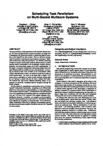
Fig. 1. Organization of Cell.
allelism requires data redistribution and incurs a high performance penalty. 3.3
Hardware Platform
The Cell BE is a heterogeneous multi-core processor which integrates a simultaneous multithreading PowerPC core ( the Power Processing Element or PPE), and eight specialized accelerator cores (the Synergistic Processing Elements or SPEs) [11]. These elements are connected in a ring topology on an on-chip network called the Element Interconnect Bus (EIB). The organization of Cell is illustrated in Figure 1. The PPE is a 64-bit SMT processor running the PowerPC ISA, with vector/SIMD multimedia extensions [1]. The PPE has two levels of on-chip cache. The L1-I and L1-D caches of the PPE have a capacity of 32 KB. The L2 cache of the PPE has a capacity of 512 KB. Each SPE is a 128-bit vector processor with two major components: a Synergistic Processor Unit (SPU) and a Memory Flow Controller (MFC). All instructions are executed on the SPU. The SPU includes 128 registers, each 128 bits wide, and 256 KB of software-controlled local storage. The SPU can fetch instructions and data only from its local storage and can write data only to its local storage. The SPU implements a Cell-specific set of SIMD intrinsics. All single precision floating point operations on the SPU are fully pipelined and the SPU can issue one single-precision floating point operation per cycle. Double precision floating point operations are partially pipelined and two double-precision floating point operations can be issued every six cycles. Double-precision FP performance is therefore significantly lower than singleprecision FP performance. With all eight SPUs active and fully pipelined double precision FP operation, the Cell BE is capable of a peak performance of 21.03 Gflops. In single-precision FP operation, the Cell BE is capable of a peak performance of 230.4 Gflops [9]. The SPE can access RAM through direct memory access (DMA) requests. 9
DMA transfers are handled by the MFC. All programs running on an SPE use the MFC to move data and instructions between local storage and main memory. Data transferred between local storage and main memory must be 128-bit aligned. The size of each DMA transfer can be at most 16 KB. DMAlists can be used for transferring more than 16 KB of data. A list can have up to 2,048 DMA requests, each for up to 16 KB. The MFC supports only DMA transfer sizes that are 1, 2, 4, 8 or multiples of 16 bytes long. The EIB is an on-chip coherent bus that handles communication between the PPE, SPE, main memory, and I/O devices. Physically, the EIB is a 4-ring structure, which can transmit 96 bytes per cycle, for a maximum theoretical memory bandwidth of 204.8 Gigabytes/second. The EIB can support more than 100 outstanding DMA requests. In this work we are using a Cell blade (IBM BladeCenter QS20) with two Cell BEs running at 3.2 GHz, and 1GB of XDR RAM (512 MB per processor). The PPEs run Linux Fedora Core 5. We use the Toolchain 4.0.2 compilers and Lam/MPI 7.1.3.
3.4
RAxML and PBPI on the Cell BE
We optimized extensively both RAxML and PBPI on the Cell BE, beginning from detailed profiling of both codes. The main guidelines for optimization were: • Offloading of major computational kernels of the codes on SPEs. • Vectorization, to exploit the SIMD units on SPEs. • Double buffering, to achieve effective overlap of communication and computation. • Alignment and localization of data with the corresponding code on the local storage of SPEs, to maximize locality. • Optimization and vectorization of branches to avoid a branch bottleneck on SPEs. • Loop-level optimizations such as unrolling and scheduling. • Use of optimized numerical implementations of linear algebra kernels, more specifically to replace the expensive double precision implementations of certain library functions with numerical implementations that leverage single precision arithmetic [21]. The actual process of porting and optimizing RAxML on Cell is described in more detail in [7]. For PBPI we followed an identical optimization process. The SPE-specific optimizations resulted in SPE code that ran more than five times faster than the SPE code that was extracted directly from the enclosing PPE code. 10
4
Scheduling Multi-Grain Parallelism on Cell
We hereby explore the possibilities for exploiting multi-grain parallelism on Cell. The Cell PPE can execute two threads or processes simultaneously, from where code can be off-loaded and executed on SPEs. To increase the sources of parallelism for SPEs, the user may consider two approaches: • The user may oversubscribe the PPE with more processes or threads, than the number of processes/threads that the PPE can execute simultaneously. In other words, the programmer attempts to find more parallelism to offload to accelerators, by attempting a more fine-grain task decomposition of the code. In this case, the runtime system needs to schedule the host processes/threads so as to minimize the time needed to off-load code to all available accelerators. We present an event-driven task-level scheduler which achieves this goal in Section 4.1. • The user can introduce a new dimension of parallelism to the application by distributing loops from within the off-loaded functions across multiple SPEs. In other words, the user can exploit data parallelism both within and across accelerators. Each SPE can work on a part of a distributed loop, which can be further accelerated with SIMDization. We present case studies that motivate the dynamic extraction of multi-grain parallelism via loop distribution in Section 4.2.
4.1
Event-Driven Task Scheduling
EDTLP is a runtime scheduling module which can be embedded transparently in MPI codes. The EDTLP scheduler operates under the assumption that the code to off-load to accelerators is specified by the user at the level of functions. In the case of Cell, this means that the user has either constructed SPE threads in a separate code module, or annotated the host PPE code with directives to extract SPE threads via a compiler [4]. The EDTLP scheduler avoids underutilization of SPEs by oversubscribing the PPE and preventing a single MPI process from monopolizing the PPE. Informally, the EDTLP scheduler off-loads tasks from MPI processes. A task ready for off-loading serves as an event trigger for the scheduler. Upon the event occurrence, the scheduler immediately attempts to serve the MPI process that carries the task to off-load and sends the task to an available SPE, if any. While off-loading a task, the scheduler suspends the MPI process that spawned the task and switches to another MPI process, anticipating that more tasks will be available for off-loading from ready-to-run MPI processes. Switching upon off-loading prevents MPI processes from blocking the PPE while waiting 11
(a)
(b)
Fig. 2. Scheduler behavior for two off-loaded tasks, representative of RAxML. Case (a) illustrates the behavior of the EDTLP scheduler. Case (b) illustrates the behavior of the Linux scheduler with the same workload. The numbers correspond to MPI processes. The shaded slots indicate context switching. The example assumes a Cell-like system with four SPEs.
for their tasks to return. The scheduler attempts to sustain a high supply of tasks for off-loading to SPEs by serving MPI processes round-robin. The downside of a scheduler based on oversubscribing a processor is contextswitching overhead. Cell in particular also suffers from the problem of interference between processes or threads sharing the SMT PPE core. The granularity of the off-loaded code determines if the overhead introduced by oversubscribing the PPE can be tolerated. The code off-loaded to an SPE should be coarse enough to marginalize the overhead of context switching performed on the PPE. The EDTLP scheduler addresses this issue by performing granularity control of the off-loaded tasks and preventing off-loading of code that does not meet a minimum granularity threshold. Figure 2 illustrates an example of the difference between scheduling MPI processes with the EDTLP scheduler and the native Linux scheduler. In this example, each MPI process has one task to off-load to SPEs. For illustrative purposes only, we assume that there are only 4 SPEs on the chip. In Figure 2(a), once a task is sent to an SPE, the scheduler forces a context switch on the PPE. Since the PPE is a two-way SMT, two MPI processes can simultaneously off-load tasks to two SPEs. The EDTLP scheduler enables the use of four SPEs via function off-loading. On the contrary, if the scheduler waits for the completion of a task before providing an opportunity to another MPI process to off-load (Figure 2 (b)), the application can only utilize two SPEs. Realistic application tasks often have significantly shorter lengths than the time quanta used by the Linux scheduler. For example, in RAxML, task lengths measure in the order of tens of microseconds, when Linux time quanta measure to tens of milliseconds. Table 1(a) compares the performance of the EDTLP scheduler to that of the native Linux scheduler, using RAxML and running a workload comprising 42 organisms. In this experiment, the number of performed bootstraps is not constant and it is equal to the number of MPI processes. The EDTLP scheduler 12
(a)
EDTLP
Linux
EDTLP
Linux
1 worker, 1 bootstrap
19.7s
19.7s
1 worker, 20,000 gen.
265s
263.5
2 workers, 2 bootstraps
22.2s
30s
2 workers, 20,000 gen.
136.1s
145
3 workers, 3 bootstraps
26s
40.7s
3 workers, 20,000 gen.
102.3
187.2
4 workers, 4 bootstraps
28.1s
43.3s
4 workers, 20,000 gen.
72.5
134.9
5 workers, 5 bootstraps
33s
60.7s
5 workers, 20,000 gen.
74.5
186.3
6 workers, 6 bootstraps
34s
61.8s
6 workers, 20,000 gen.
56.2
146.3
7 workers, 7 bootstraps
38.8s
81.2s
7 workers, 20,000 gen.
60.1
157.8
8 workers, 8 bootstraps
39.8s
81.7s
8 workers, 20,000 gen.
57.6
158.3
(b)
Table 1 Performance comparison for (a) RAxML and (b) PBPI with two schedulers. The second column shows execution time with the EDTLP scheduler. The third column shows execution time with the native Linux kernel scheduler. The workload for RAxML contains 42 organisms. The workload for PBPI contains 107 organisms.
outperforms the Linux scheduler by up to a factor of 2.7. In the experiment with PBPI, we execute the code with one Markov chain for 20,000 generations and we change the number of MPI processes used across runs. The workload for PBPI includes 107 organisms. Since the amount of work is constant, execution time should drop as the number of processes increases. EDTLP outperforms the Linux scheduler policy in PBPI by up to a factor of 2.7.
4.2
Dynamic Loop Scheduling
When the degree of task-level parallelism is less than the number of available SPEs, the runtime system may activate a second dimension of data parallelism, by distributing loops encapsulated in tasks between SPEs. We implemented a micro-tasking library for dynamically parallelizing loops on Cell. The microtasking library enables loop distribution across a variable number of SPEs and provides the required data consistency and synchronization mechanisms. The parallelization scheme of the microtasking library is outlined in Figure 3. The program is executed on the PPE until the execution reaches the parallel loop to be off-loaded. At that point the PPE sends a signal to a single SPE which is designated as the master. The signal is processed by the master and further broadcasted to all workers involved in parallelization. Upon a signal reception, each SPE worker fetches the data necessary for loop execution. We ensure that SPEs work on different parts of the loop and do not overlap by assigning a unique identifier to each SPE thread involved in parallelization of the loop. Global data, changed by any of the SPEs during loop execution, is committed to main memory at the end of each iteration. After processing the assigned parts of the loop, the SPE workers send a notification back to the master. If the loop includes a reduction, the master collects also partial results from the SPEs and accumulates them locally. All communication between SPEs is performed on chip in order to avoid the long latency of communicating through shared memory. 13
Master Worker1
Worker7 Master sending start signal to Worker7
Master sending start signal to Worker1 Master Worker1 executes executes iterations iterations from 1 to x/8 from x/8 to x/4
Worker7 executes
. . .
iterations from 7/8x to x
Worker1 sending stop signal to Master Worker7 sending stop signal to Master Total number
x −of iterations
Fig. 3. Parallelizing a loop across SPEs using a work-sharing model with an SPE designated as the master.
Note that in our loop parallelization scheme on Cell, all work performed by the master SPE can also be performed by the PPE. In this case, the PPE would broadcast a signal to all SPE threads involved in loop parallelization and the partial results calculated by SPEs would be accumulated back at the PPE. Such collective operations increase the frequency of SPE-PPE communication, especially when the distributed loop is a nested loop. In the case of RAxML, in order to reduce SPE-PPE communication and avoid unnecessary invocation of the MPI process that spawned the parallelized loop, we opted to use an SPE to distribute loops to other SPEs and collect the results from other SPEs. In PBPI, we let the PPE execute the master thread during loop parallelization, since loops are coarse enough to overshadow the loop execution overhead. Optimizing and selecting between these loop execution schemes is a subject of ongoing research. SPE threads participating in loop parallelization are created once upon offloading the code for the first parallel loop to SPEs. The threads remain active and pinned to the same SPEs during the entire program execution, unless the scheduler decides to change the parallelization strategy and redistribute the SPEs between one or more concurrently executing parallel loops. Pinned SPE threads can run multiple off-loaded loop bodies, as long as the code of these loop bodies fits on the local storage of the SPEs. If the loop parallelization strategy is changed on the fly by the runtime system, a new code module with loop bodies that implement the new parallelization strategy is loaded on the local storage of the SPEs. Table 2 illustrates the performance of the basic loop-level parallelization scheme of our runtime system in RAxML. Table 2(a) illustrates the execution time 14
of RAxML using one MPI process and performing one bootstrap, on a data set which comprises 42 organisms. This experiment isolates the impact of our loop-level parallelization mechanisms on Cell. The number of iterations in parallelized loops depends on the size of the input alignment in RAxML. For the given data set, each parallel loop executes 228 iterations.
(a)
1 worker, 1 boot., no LLP
19.7s
1 worker, 1 boot., no LLP
47.9s
1 worker, 1 boot., 2 SPEs used for LLP
14s
1 worker, 1 boot., 2 SPEs used for LLP
29.5s
1 worker, 1 boot., 3 SPEs used for LLP
13.36s
1 worker, 1 boot., 3 SPEs used for LLP
23.3s
1 worker, 1 boot., 4 SPEs used for LLP
12.8s
1 worker, 1 boot., 4 SPEs used for LLP
20.5s
1 worker, 1 boot., 5 SPEs used for LLP
13.8s
1 worker, 1 boot., 5 SPEs used for LLP
18.7s
1 worker, 1 boot., 6 SPEs used for LLP
12.47s
1 worker, 1 boot., 6 SPEs used for LLP
18.1s
1 worker, 1 boot., 7 SPEs used for LLP
11.4s
1 worker, 1 boot., 7 SPEs used for LLP
17.1s
1 worker, 1 boot., 8 SPEs used for LLP
11.44s
1 worker, 1 boot., 8 SPEs used for LLP
16.8s
(b)
Table 2 Execution time of RAxML when loop-level parallelism (LLP) is exploited in one bootstrap, via work distribution between SPEs. The input file is 42 SC: (a) DNA sequences are represented with 10,000 nucleotides, (b) DNA sequences are represented with 20,000 nucleotides.
The results shown in Table 2(a) suggest that when using loop-level parallelism RAxML sees a reasonable yet limited performance improvement. The highest speedup (1.72) is achieved with 7 SPEs. The reasons for the modest speedup are the non-optimal coverage of loop-level parallelism —more specifically, less than 90% of the original sequential code is covered by parallelized loops—, the fine granularity of the loops, and the fact that most loops have reductions, which create bottlenecks on the Cell DMA engine. The performance degradation that occurs when 5 or 6 SPEs are used, happens because of specific memory alignment constraints that have to be met on the SPEs. It is due to alignment constraints that in certain occasions it is not possible to evenly distribute the data used in the loop body and therefore the workload of iterations between SPEs. More specifically, the use of character arrays for the main data set in RAxML forces array transfers in multiples of 16 array elements. Consequently, loop distribution across processors is done with a minimum chunk size of 16 iterations. Loop-level parallelization in RAxML can achieve higher speedup in a single bootstrap with larger input data sets. Alignments that have a larger number of nucleotides per organism have more loop iterations to distribute across SPEs. To illustrate the behavior of loop-level parallelization with coarser loops, we repeated the previous experiment using a data set where the DNA sequences are represented with 20,000 nucleotides. The results are shown in Table 2(b). The loop-level parallelization scheme scales gracefully to 8 SPEs in this experiment. PBPI exhibits clearly better scalability than RAxML with LLP, since the granularity of loops is coarser in PBPI than RAxML. Table 3 illustrates the 15
execution times when PBPI is executed with a variable number of SPEs used for LLP. Again, we control the granularity of the off-loaded code by using different data sets: Table 3(a) shows execution times for a data set that contains 107 organisms, each represented by a DNA sequence of 3,000 nucleotides. Table 3(b) shows execution times for a data set that contains 107 organisms, each represented by a DNA sequence of 10,000 nucleotides. We run PBPI with one Markov chain for 20,000 generations. For the two data sets, PBPI achieves a maximum speedup of 4.6 and 6.1 respectively, after loop-level parallelization.
(a)
1 worker, 1,000 gen., no LLP
27.2s
1 worker, 20,000 gen., no LLP
262s
1 worker, 1,000 gen., 2 SPEs used for LLP
14.9s
1 worker, 20,000 gen., 2 SPEs used
131.3s
1 worker, 1,000 gen., 3 SPEs used for LLP
11.3s
1 worker, 20,000 gen., 3 SPEs used
92.3s
1 worker, 1,000 gen., 4 SPEs used for LLP
8.4s
1 worker, 20,000 gen., 4 SPEs used
70.1s
1 worker, 1,000 gen., 5 SPEs used for LLP
7.3s
1 worker, 20,000 gen., 5 SPEs used
58.1s
1 worker, 1,000 gen., 6 SPEs used for LLP
6.8s
1 worker, 20,000 gen., 6 SPEs used
49s
1 worker, 1,000 gen., 7 SPEs used for LLP
6.2s
1 worker, 20,000 gen., 7 SPEs used
43s
1 worker, 1,000 gen., 8 SPEs used for LLP
5.9s
1 worker, 20,000 gen., 8 SPEs used
39.7s
(b)
Table 3 Execution time of PBPI when loop-level parallelism (LLP) is exploited via work distribution between SPEs. The input file is 107 SC: (a) DNA sequences are represented with 1,000 nucleotides, (b) DNA sequences are represented with 10,000 nucleotides.
5
MGPS: Dynamic Scheduling of Task- and Loop-Level Parallelism
Merging task-level and loop-level parallelism on Cell can improve the utilization of accelerators. A non-trivial problem with such a hybrid parallelization scheme is the assignment of accelerators to tasks. The optimal assignment is largely application-specific, task-specific and input-specific. We support this argument using RAxML as an example. The discussion in this section is limited to RAxML, where the degree of outermost parallelism can be changed arbitrarily by varying the number of MPI processes executing bootstraps, with a small impact on performance. PBPI uses a data decomposition approach which depends on the number of processors, therefore dynamically varying the number of MPI processes executing the code at runtime can not be accomplished without data redistribution or excessive context switching and process control overhead.
5.1
Application-Specific Hybrid Parallelization on Cell
We present a set of experiments with RAxML performing a number of bootstraps ranging between 1 and 128. In these experiments we use three versions of RAxML. Two of the three versions use hybrid parallelization models combining task- and loop-level parallelism. The third version exploits only task-level 16
1000 900
EDTLP+LLP with 4 SPEs per parallel loop EDTLP+LLP with 2 SPEs per parallel loop EDTLP
100
Execution time (s)
Execution time (s)
120
80
60
40
20
EDTLP+LLP 4 SPEs per parallel loop EDTLP+LLP 2 SPEs per parallel loop EDTLP
800 700 600 500 400 300 200 100 0
0 1
2
3
4
5
6
7
8
9
10
11
12
13
14
15
0
16
20
40
60
80
100
120
140
Number of bootstraps
Number of bootstraps
(a)
(b)
Fig. 4. Comparison of task-level and hybrid parallelization schemes in RAxML, on the Cell BE. The input file is 42 SC. The number of ML trees created is (a) 1–16, (b) 1–128.
parallelism and uses the EDTLP scheduler. More specifically, in the first version, each off-loaded task is parallelized across 2 SPEs, and 4 MPI processes are multiplexed on the PPE, executing 4 concurrent bootstraps. In the second version, each off-loaded task is parallelized across 4 SPEs and 2 MPI processes are multiplexed on the PPE, executing 2 concurrent bootstraps. In the third version, the code concurrently executes 8 MPI processes, the off-loaded tasks are not parallelized and the tasks are scheduled with the EDTLP scheduler. Figure 4 illustrates the results of this experiment, with a data set representing 42 organisms. The x-axis shows the number of bootstraps, while the y-axis shows execution time in seconds. As expected, the hybrid model outperforms EDTLP when up to 4 bootstraps are executed, since only a combination of EDTLP and LLP can off-load code to more than 4 SPEs simultaneously. With 5 to 8 bootstraps, the hybrid models execute bootstraps in batches of 2 and 4 respectively, while the EDTLP model executes all bootstraps in parallel. EDTLP activates 5 to 8 SPEs solely for task-level parallelism, leaving room for loop-level parallelism on at most 3 SPEs. This proves to be unnecessary, since the parallel execution time is determined by the length of the non-parallelized off-loaded tasks that remain on at least one SPE. In the range between 9 and 12 bootstraps, combining EDTLP and LLP selectively, so that the first 8 bootstraps execute with EDTLP and the last 4 bootstraps execute with the hybrid scheme is the best option. For the input data set with 42 organisms, performance of EDTLP and hybrid EDTLP-LLP schemes is almost identical when the number of bootstraps is between 13 and 16. When the number of bootstraps is higher than 16, EDTLP clearly outperforms any hybrid scheme (Figure 4(b)). The reader may notice that the problem of hybrid parallelization is trivialized when the problem size is scaled beyond a certain point, which is 28 bootstraps in the case of RAxML (see Section 5.2). A production run of RAxML for 17
real-world phylogenetic analysis would require up to 1,000 bootstraps, thus rendering hybrid parallelization seemingly unnecessary. However, if a production RAxML run with 1,000 bootstraps were to be executed across multiple Cell BEs, and assuming equal division of bootstraps between the processors, the cut-off point for EDTLP outperforming the hybrid EDTLP-LLP scheme would be set at 36 Cell processors. Beyond this scale, performance per processor would be maximized only if LLP were employed in conjunction with EDTLP on each Cell. Although this observation is empirical and somewhat simplifying, it is further supported by the argument that scaling across multiple processors will in all likelihood increase communication overhead and therefore favor a parallelization scheme with less MPI processes. The hybrid scheme reduces the volume of MPI processes compared to the pure EDTLP scheme, when the granularity of work per Cell becomes fine.
5.2
MGPS
The purpose of MGPS is to dynamically adapt the parallel execution by either exposing only one layer of task parallelism to the SPEs via event-driven scheduling, or expanding to a second layer of data parallelism and merging it with task parallelism when SPEs are underutilized at runtime. MGPS extends the EDTLP scheduler with an adaptive processor-saving policy. The scheduler runs locally in each process and it is driven by two events: • arrivals, which correspond to off-loading functions from PPE processes to SPE threads; • departures, which correspond to completion of SPE functions. MGPS is invoked upon arrivals and departures of tasks. Initially, upon arrivals, the scheduler conservatively assigns one SPE to each off-loaded task. Upon a departure, the scheduler monitors the degree of task-level parallelism exposed by each MPI process, i.e. how many discrete tasks were off-loaded to SPEs while the departing task was executing. This number reflects the history of SPE utilization from task-level parallelism and is used to switch from the EDTLP scheduling policy to a hybrid EDTLP-LLP scheduling policy. The scheduler monitors the number of SPEs that execute tasks over epochs of 100 off-loads. If the observed SPE utilization is over 50% the scheduler maintains the most recently selected scheduling policy (EDTLP or EDTLP-LLP). If the observed SPE utilization falls under 50% and the scheduler uses EDTLP, it switches to EDTLP-LLP by loading parallelized versions of the loops in the local storages of SPEs and performing loop distribution. To switch between different parallel execution models at runtime, the runtime system uses code versioning. It maintains three versions of the code of each 18
1000 MGPS EDTLP+LLP with 4 SPEs per parallel loop EDTLP+LLP with 2 SPEs per parallel loop EDTLP
100
MGPS EDTLP+LL with 4 SPEs per parallel loop EDTLP+LLP with 2 SPEs per parallel loop EDTLP
900
Execution time (s)
Execution time (s)
120
80
60
40
20
800 700 600 500 400 300 200 100 0
0 1
2
3
4
5
6
7
8
9
10
11
12
13
14
15
0
16
20
40
60
80
100
120
140
Number of bootstraps
Number of bootstraps
(a)
(b)
Fig. 5. Comparison between MGPS, EDTLP and static EDTLP-LLP. The input file is 42 SC. The number of ML trees created is (a) 1–16, (b) 1–128. The lines of MGPS and EDTLP overlap completely in (b).
task. One version is used for execution on the PPE. A second version is used for execution on an SPE from start to finish, using SIMDization to exploit the vector execution units of the SPE. The third version is used for distribution of the loop enclosed by the task between more than one SPEs. The use of code versioning increases code management overhead, as SPEs may need to load different versions of the code of each off-loaded task at runtime. On the other hand, code versioning obviates the need for conditionals that would be used in a monolithic version of the code. These conditionals are expensive on SPEs, which lack branch prediction capabilities. Our experimental analysis indicates that overlaying code versions on the SPEs via code transfers ends up being slightly more efficient than using monolithic code with conditionals. This happens because of the overhead and frequency of the conditionals in the monolithic version of the SPE code, but also because the code overlays leave more space available in the local storage of SPEs for data caching and buffering to overlap computation and communication [7]. We compare MGPS to EDTLP and two static hybrid (EDTLP-LLP) schedulers, using 2 SPEs per loop and 4 SPEs per loop respectively. Figure 5 shows the execution times of MGPS, EDTLP-LLP and EDTLP with various RAxML workloads. The x-axis shows the number of bootstraps, while the y-axis shows execution time. We observe benefits from using MGPS for up to 28 bootstraps. Beyond 28 bootstraps, MGPS converges to EDTLP and both are increasingly faster than static EDTLP-LLP execution, as the number of bootstraps increases. A clear disadvantage of MGPS is that the time needed for any adaptation decision depends of the total number of off-loading requests, which in turn is inherently application-dependent and input-dependent. If the off-loading requests from different processes are spaced apart, there may be extended idle periods on SPEs, before adaptation takes place. A second disadvantage of MGPS is that its dynamic scheduling policy depends on the initial configura19
tion used to execute the application. In RAxML, MGPS converges to the best execution strategy only if the application begins by oversubscribing the PPE and exposing the maximum degree of task-level parallelism to the runtime system. This strategy is unlikely to converge to the best scheduling policy in other applications, where task-level parallelism is limited and data parallelism is more dominant. In this case, MGPS would have to commence its optimization process from a different program configuration favoring data-level rather than task-level parallelism. PBPI is an application where MGPS does not converge to the optimal solution. We address the aforementioned shortcomings via a sampling-based MGPS algorithm (S-MGPS), which we introduce in the next section.
6
S-MGPS
We begin this section by presenting a motivating example to show why controlling concurrency on the Cell is useful, even if SPEs are seemingly fully utilized. This example motivates the introduction of a sampling-based algorithm that explores the space of program and system configurations that utilize all SPEs, under different distributions of SPEs between concurrently executing tasks and parallel loops. We present S-MGPS and evaluate S-MGPS using RAxML and PBPI.
6.1
Motivating Example
Increasing the degree of task parallelism on Cell comes at a cost, namely increasing contention between MPI processes that time-share the PPE. Pairs of processes that execute in parallel on the PPE suffer from contention for shared resources, a well-known problem of simultaneous multithreaded processors. Furthermore, with more processes, context switching overhead and lack of co-scheduling of SPE threads and PPE threads from which the SPE threads originate, may harm performance. On the other hand, while looplevel parallelization can ameliorate PPE contention, its performance benefit depends on the granularity and locality properties of parallel loops. Figure 6 shows the efficiency of loop-level parallelism in RAxML when the input data set is relatively small. The input data set in this example (25 SC) has 25 organisms, each of them represented by a DNA sequence of 500 nucleotides. In this experiment, RAxML is executed multiple times with a single worker process and a variable number of SPEs used for LLP. The best execution time is achieved with 5 SPEs. The behavior illustrated in Figure 6 is caused by several factors, including the granularity of loops relative to the overhead of 20
50
Exeutin time (s)
45 40 35 30 25 20 15 10 5 0 1
2
3
4
5
6
7
8
Number of SPEs
Fig. 6. Execution time of RAxML with a variable number of SPE threads. The input dataset is 25 SC. 400
Execution time (s)
350
8 worker processes, 1 SPE per off-loaded task 4 worker processes, 2SPEs per off-loaded task
300
2 worker processes, 4 SPEs per off-loaded task
250 200 150 100 50 0 0
20
40
60
80
100
120
140
Number of bootstraps
Fig. 7. Execution times of RAxML, with various static multi-grain scheduling strategies. The input dataset is 25 SC.
PPE-SPE communication and load imbalance (discussed in Section 4.2). By using two dimensions of parallelism to execute an application, the runtime system can control both PPE contention and loop-level parallelization overhead. Figure 7 illustrates an example in which multi-grain parallel executions outperform one-dimensional parallel executions in RAxML, for any number of bootstraps. In this example, RAxML is executed with three static parallelization schemes, using 8 MPI processes and 1 SPE per process, 4 MPI processes and 2 SPEs per process, or 2 MPI processes and 4 SPEs per process respectively. The input data set is 25 SC. RAxML performs the best in this data set with a multi-level parallelization model when 4 MPI processes are simultaneously executed on the PPE and each of them uses 2 SPEs for loop-level parallelization.
6.2
A Sampling-Based Scheduler for Multi-grain Parallelism
The S-MGPS scheduler automatically determines the best parallelization scheme for a specific workload, by using a sampling period. During the sampling pe21
riod, S-MGPS performs a search of program configurations along the available dimensions of parallelism. The search starts with a single MPI process and during the first step S-MGPS determines the optimal number of SPEs that should be used by a single MPI process. The search is implemented by sampling execution phases of the MPI process with different degrees of loop-level parallelism. The execution phases are delimited by SPE tasks and global synchronization operations. Phases represent code that is executed repeatedly in an application and dominates execution time. Although we identify phases manually in our execution environment, the selection process for phases is trivial and can be automated in a compiler. Furthermore, parallel applications almost always exhibit a very strong runtime periodicity in their execution patterns, which makes the process of isolating the dominant execution phases straightforward. Automation of the phase identification process by a compiler is left as future work. Once the first sampling step of S-MGPS is completed, the search continues by sampling execution intervals with every feasible combination of task-level and loop-level parallelism. In the second phase of the search, the degree of loop-level parallelism never exceeds the optimal value determined by the first sampling step. For each execution interval, the scheduler uses execution time of phases as a criterion for selecting the optimal dimension(s) and granularity of parallelism per dimension. S-MGPS uses a performance-driven mechanism to rightsize parallelism on Cell, as opposed to the utilization-driven mechanism used in MGPS. Figure 8 illustrates the steps of the sampling phase when 2 MPI processes are executed on the PPE. This process can be performed for any number of MPI processes that can be executed on a single Cell node. For each MPI process, the runtime system uses a variable number of SPEs, ranging from 1 up to the optimal number of SPEs determined by the first phase of sampling. The purpose of the sampling period is to determine the configuration of parallelism that maximizes efficiency. We define a throughput metric W as: W =
C T
(1)
where C is the number of completed tasks and T is execution time. Note that a task is defined as a function off-loaded on SPEs, therefore C captures application- and input-dependent behavior. S-MGPS computes C by counting the number of task off-loads. This metric works reasonably well, assuming that tasks of the same type (i.e. the same function off-loaded multiple times on an SPE) have approximately the same execution time. This is indeed the case in the applications that we studied. The metric can be easily extended so that each task is weighed with its execution time relative to the execution time 22
SPE5
SPE6
SPE7
SPE8
SPE5
Process1
SPE6
SPE7
SPE8
Process1
PPE
PPE
EIB
Process2
EIB
Process2 SPE1
SPE2
SPE3
SPE4
SPE1
SPE2
(a) SPE5
SPE6
SPE3
SPE4
(b) SPE7
SPE8
SPE5
Process1
SPE6
SPE7
SPE8
Process1
PPE
PPE
EIB
Process2
EIB
Process2 SPE1
SPE2
SPE3
SPE4
SPE1
(c)
SPE2
SPE3
SPE4
(d)
Fig. 8. The sampling phase of S-MGPS. Samples are taken from four execution intervals, during which the code performs identical operations. For each sample, each MPI process uses a variable number of SPEs to parallelize its enclosed loops.
of other tasks, to account for unbalanced task execution times. We do not explore this option further in this paper. S-MGPS calculates efficiency for every sampled configuration and selects the configuration with the maximum efficiency for the rest of the execution. In Table 4 we represent partial results of the sampling phase in RAxML for different input datasets. In this example, the degree of task-level parallelism sampled is 8, 4 and 2, while the degree of loop-level parallelism sampled is 1, 2 and 4. In the case of RAxML we set a single sampling phase to be time necessary for all active worker processes to finish a single bootstrap. Therefore, in the case of RAxML in Table 4, the number of bootstraps and the execution time differ across sampling phases: when the number of active workers is 8, the sampling phase will contain 8 bootstraps, when the number of active workers is 4 the sampling phase will contain 4 bootstraps, etc. Nevertheless, the throughput (W ) remains invariant across different sampling phases and always represents the efficiency of a certain configuration, i.e. amount of work done per second. Results presented in Table 4 and Figures 7 and 4(b) confirm that S-MGPS converges to the optimal configuration for the input files 25 SC and 42 SC. Since the scheduler performs an exhaustive search, for the 25 SC input, the total number of tested configurations during the sampling period on Cell is 23
deg(TLP) ×
# bootstr. per
# off-loaded
phase
deg (LLP)
sampling phase
tasks
duration time
42 SC
8x1
8
2,526,126
41.73s
60,535
42 SC
4x2
4
1,263,444
21.05s
60,021
42 SC
2x4
2
624,308
14.42s
43,294
25 SC
8x1
8
1,261,232
16.53s
76,299
25 SC
4x2
4
612,155
8.01s
76,423
Dataset
W
25 SC 2x4 2 302,394 5.6s 53,998 Table 4 Efficiency of different program configurations with two data sets in RAxML. The best configuration for 42 SC input is deg(TLP)=8, deg(LLP)=1. The best configuration for 25 SC is deg(TLP)=4, deg(LLP)=2. deg() corresponds the degree of a given dimension of parallelism (LLP or TLP).
17, for up to 8 MPI processes and 1 to 5 SPEs used per MPI process for looplevel parallelization. The upper bound of 5 SPEs per loop is determined by the first phase of the sampling period (Figure 6). Assuming that performance is optimized if the maximum number of SPEs of the processor are involved in parallelization, the feasible configurations to sample are constrained by deg(TLP)×deg(LLP)=8, for a single Cell with 8 SPEs. Under this constraint, the number of samples needed by S-MGPS on Cell drops to 3. Unfortunately, when considering only configurations that use all SPEs, the scheduler may omit a configuration that does not use all SPEs but still performs better than the best scheme that uses all processor cores. In principle, this situation may occur in certain non-scalable codes. To address such cases, we recommend the use of exhaustive search in S-MGPS, given that the total number of feasible configurations of SPEs on a Cell is manageable and small compared to the number of tasks and the number of instances of each task executed in real applications. This assumption may need to be revisited in the future for largescale systems with many cores and exhaustive search may need to be replaced by heuristics such as hill climbing or simulated annealing. In Table 5 we compare the performance of S-MGPS to the static scheduling policies with both one-dimensional (TLP) and multi-grain (TLP-LLP) parallelism on Cell, using RAxML. For a small number of bootstraps, S-MGPS underperforms the best static scheduling scheme by 10%. The reason is that S-MGPS expends a significant percentage of execution time in the sampling period, while executing the program in mostly suboptimal configurations. As the number of bootstraps increases, S-MGPS comes closer to the performance of the best static scheduling scheme (within 3%–5%). To map PBPI to Cell, we used a hybrid parallelization approach where a 24
deg(TLP)=8,
deg(TLP)=4,
deg(TLP)=1,
deg(LLP)=1
deg(LLP)=2
deg(LLP)=4
S-MGPS
32 boots.
60s
57s
80s
63s
64 boots.
117s
112s
161s
118s
128 boots. 231s 221s 323s 227s Table 5 RAxML – Comparison between S-MGPS and static scheduling schemes, illustrating the convergence overhead of S-MGPS.
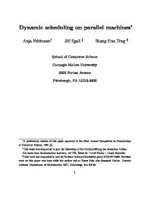
fixed number of MPI processes is multiplexed on the PPE and multiple SPEs are used for loop-level parallelization. The performance of the parallelized off-loaded code in PBPI is influenced by the same factors as in RAxML: granularity of the off-loaded code, PPE-SPE communication, and load imbalance. In Figure 9 we present the performance of PBPI when a variable number of SPEs is used to execute the parallelized off-loaded code. The input file we used in this experiment is 107 SC, including 107 organisms, each represented by a DNA sequence of 1,000 nucleotides. We run PBPI with one Markov chain for 200,000 generations. Figure 9 contains four executions of PBPI with 1, 2, 4 and 8 MPI processes with 1–16, 1–8, 1–4 and 1–2 SPEs used per MPI process respectively. In all experiments we use a single BladeCenter with two Cell BE processors (total of 16 SPEs). In the experiments with 1 and 2 MPI processes, the off-loaded code scales successfully only up to a certain number of SPEs, which is always smaller than the number of total available SPEs. Furthermore, the best performance in these two cases is reached when the number of SPEs used for parallelization is smaller than the total number of available SPEs. The optimal number of SPEs in general depends on the input data set and on the outermost parallelization and data decomposition scheme of PBPI. The best performance for the specific dataset is reached by using 4 MPI processes, spread across 2 Cell BEs, with each process using 4 SPEs on one Cell BE. This optimal operating point shifts with different data set sizes. The fixed virtual processor topology and data decomposition method used in PBPI prevents dynamic scheduling of MPI processes at runtime without excessive overhead. We have experimented with the option of dynamically changing the number of active MPI processes via a gang scheduling scheme, which keeps the total number of active MPI processes constant, but co-schedules MPI processes in gangs of size 1, 2, 4, or 8 on the PPE and uses 8, 4, 2, or 1 SPE(s) per MPI process respectively, for the execution of parallel loops. This scheme also suffered from system overhead, due to process control and context switching on the SPEs. Pending better solutions for adaptively controlling the number of processes in MPI, we evaluated S-MGPS in several scenarios where the number of MPI processes remains fixed. Using S-MGPS we were able to determine 25
Execution time (s)
600
1 MPI process 2 MPI processes 4 MPI processes 8 MPI processes
500
400
300
200
100
0 1
2
3
4
5
6
7
8
9
10
11
12
13
14
15
16
Number of SPEs
Fig. 9. PBPI executed with different levels of TLP and LLP parallelism: deg(TLP)=1-4, deg(LLP)=1–16
the optimal degree of loop-level parallelism, for any given degree of task-level parallelism (i.e. initial number of MPI processes) in PBPI. Being able to pinpoint the optimal SPE configuration for LLP is still important since different loop parallelization strategies can result in a significant difference in execution time. For example, the na¨ıve parallelization strategy, where all available SPEs are used for parallelization of off-loaded loops, can result in up to 21% performance degradation (see Figure 9). Table 6 shows a comparison of execution times when S-MGPS is used and when different static parallelization schemes are used. S-MGPS performs within 2% of the optimal static parallelization scheme. S-MGPS also performs up to 20% better than the na¨ıve parallelization scheme where all available SPEs are used for LLP (see Table 6(b)).
7
Conclusions
We investigated the problem of scheduling dynamic multi-dimensional parallelism on heterogeneous multi-core processors. We used the Cell BE as a case study and as a timely and relevant high-performance computing platform. Our main contribution is a feedback-guided dynamic scheduler, S-MGPS, which rightsizes multi-dimensional parallelism automatically and improves upon earlier proposals for event-driven scheduling of task-level parallelism (EDTLP) and utilization-driven scheduling of multi-grain parallelism (MGPS) on the Cell BE. S-MGPS searches for optimal configurations of multi-grain parallelism in a space of configurations which is unexplored by both EDTLP and MGPS. The scheduler uses sampling of dominant execution phases to converge to the optimal configuration and our results show that S-MGPS performs within 2%–10% off the optimal multi-grain parallelization scheme, without a-priori knowledge 26
deg(LLP)
(a)
deg(TLP)=1
1
2
3
4
5
6
7
8
Time
502
267.8
222.8
175.8
142.1
118.6
108.1
134.3
deg(TLP)=1
9
10
11
12
13
14
15
16
Time (s)
122
111.9
138.3
109.2
122.3
133.2
115.3
116.5
S-MGPS Time (s)
110.3
deg(LLP) (b)
deg(TLP)=2
1
2
3
4
5
6
7
8
Time (s)
275.9
180.8
139.4
113.5
91.3
97.3
102.55
115
S-MGPS Time (s)
93
deg(LLP) (c)
deg(LLP)
deg(TLP)=4
1
2
3
4
Time (s)
180.6
118.67
94.63
83.61
S-MGPS Time (s)
85.9
(d)
deg(TLP)=8
1
2
Time (s)
355.5
265
S-MGPS Time (s)
267
Table 6 PBPI – comparison between S-MGPS and static scheduling schemes: (a) deg(TLP)=1, deg(LLP)=1–16; (b) deg(TLP)=2, deg(LLP)=1–8; (c) deg(TLP)=4, deg(LLP)=1–4; (d) deg(TLP)=8, deg(LLP)=1–2.
of application properties. We have demonstrated the motivation and effectiveness of using S-MGPS with two complete and realistic applications from the area of computational phylogenetics, RAxML and PBPI.
Our results corroborate the need for dynamic and adaptive user-level schedulers for parallel programming on heterogeneous multi-core processors and provide motivation for further research in the area. Potential avenues that we plan to explore in the future are the extension of the three schedulers (SMGPS, MGPS, EDTLP) to incorporate inter-node communication, extension of the dynamic scheduling heuristics to account for load imbalance and task heterogeneity, and further experimentation with regular and irregular applications. We also intend to integrate S-MGPS with adaptive and threaded MPI frameworks, to minimize the overheads of adaptation of the number of MPI processes at runtime and allow S-MGPS to explore the full search space of program configurations. This effort will also involve an exploration of heuristics to prune the search space, for platforms with a large number of feasible configurations (e.g. Cell multiprocessors with many Cell BEs or large-scale Cell BE clusters). 27
Acknowledgments
This research is supported by the National Science Foundation (Grant CCR0346867), the U.S. Department of Energy (Grant DE-FG02-06ER25751), the Swiss Confederation Funding, the Barcelona Supercomputing Center, and the College of Engineering at Virginia Tech. We thank Georgia Institute of Technology, its Sony-Toshiba-IBM Center of Competence, and the National Science Foundation, for the use of Cell Broadband Engine resources that have contributed to this research. We thank Xizhou Feng and Kirk Cameron for providing us with the MPI version of PBPI. We are also grateful to the anonymous reviewers for their constructive feedback on earlier versions of this paper.
References
[1] PowerPC Microprocessor Family: Vector/SIMD Multimedia Extension Technology Programming Environments Manual. http:// www-306.ibm.com / chips / techlib. [2] D. Bader, V. Agarwal, and K. Madduri. On the Design and Analysis of Irregular Algorithms on the Cell Processor: A Case Study on List Ranking. In Proc. of the 21st International Parallel and Distributed Processing Symposium, Long Beach, CA, March 2007. [3] D.A. Bader, B.M.E. Moret, and L. Vawter. Industrial applications of highperformance computing for phylogeny reconstruction. In Proc. of SPIE ITCom, volume 4528, pages 159–168, 2001. [4] P. Bellens, J. Perez, R. Badia, and J. Labarta. Cellss: A programming model for the cell be architecture. In Proc. of Supercomputing’2006, Tampa, FL, November 2006. [5] Carsten Benthin, Ingo Wald, Michael Scherbaum, and Heiko Friedrich. Ray Tracing on the CELL Processor. Technical Report, inTrace Realtime Ray Tracing GmbH, No inTrace-2006-001 (submitted for publication), 2006. [6] Filip Blagojevic, Dimitrios S. Nikolopoulos, Alexandros Stamatakis, and Christos D. Antonopoulos. Dynamic Multigrain Parallelization on the Cell Broadband Engine. In Proc. of the 12th ACM SIGPLAN Symposium on Principles and Practice of Parallel Programming, pages 90–100, San Jose, CA, March 2007. [7] Filip Blagojevic, Alexandros Stamatakis, Christos D. Antonopoulos, and Dimitrios S. Nikolopoulos. RAxML-Cell: Parallel Phyolgenetic Tree Construction on the Cell Broadband Engine. In Proc. of the 21st IEEE/ACM International Parallel and Distributed Processing Symposium, Long Beach, CA, March 2007.
28
[8] T. Chen, K. O’Brien, and K. O’Brien. Optimizing the Use of Static Buffers for DMA on a Cell Chip. In Proc. of the 19th International Workshop on Languages and Compilers for Parallel Computing, New Orleans, LA, November 2006. [9] Thomas Chen, Ram Raghavan, Jason Dale, and Eiji Iwata. Cell broadband engine architecture and its first implementation. IBM developerWorks, Nov 2005. [10] A. E. Eichenberger et al. Optimizing Compiler for a Cell processor. Parallel Architectures and Compilation Techniques, September 2005. [11] B. Flachs et al. The Microarchitecture of the Streaming Processor for a CELL Processor. Proceedings of the IEEE International Solid-State Circuits Symposium, pages 184–185, February 2005. [12] K. Fatahalian et al. Sequoia: Programming the memory hierarchy. In Proc. of Supercomputing’2006, Tampa, FL, November 2006. [13] J. Felsenstein. Evolutionary trees from DNA sequences: A maximum likelihood approach. Journal of Molecular Evolution, 17:368–376, 1981. [14] X. Feng, K. Cameron, and D. Buell. PBPI: a high performance Implementation of Bayesian Phylogenetic Inference. In Proc. of Supercomputing’2006, Tampa, FL, November 2006. [15] X. Feng, K. Cameron, B. Smith, and C. Sosa. Building the Tree of Life on Terascale Systems. In Proc. of the 21st International Parallel and Distributed Processing Symposium, Long Beach, CA, March 2007. [16] Xizhou Feng, Duncan A. Buell, John R. Rose, and Peter J. Waddell. Parallel algorithms for bayesian phylogenetic inference. Journal of Parallel Distributed Computing, 63(7-8):707–718, 2003. [17] M. Gordon, W. Thies, and S. Amarasinghe. Exploiting Coarse-Grained Task, Data and Pipelined Parallelism in Stream Programs. In Proc. of the 12th International Conference on Architectural Support for Programming Languages and Operating Systems, pages 151–162, San Jose, CA, October 2006. [18] Nils Hjelte. Smoothed particle hydrodynamics on the cell broadband engine. Master’s thesis, Ume˚ a University, Department of Computer Science, Jun 2006. [19] IBM. Cbe tutorial v1.1. 2006. [20] Mike Kistler, Michael Perrone, and Fabrizio Petrini. Cell Multiprocessor Interconnection Network: Built for Speed. IEEE Micro, 26(3), May-June 2006. Available from http:// hpc.pnl.gov / people / fabrizio / papers / ieeemicrocell.pdf. [21] Julie Langou, Julien Langou, Piotr Luszczek, Jakub Kurzak, Alfredo Buttari, and Jack Dongarra. Exploiting the performance of 32 bit floating point arithmetic in obtaining 64 bit accuracy (revisiting iterative refinement for linear systems). In SC ’06: Proceedings of the 2006 ACM/IEEE conference on Supercomputing, page 113, New York, NY, USA, 2006. ACM Press.
29
[22] F. Petrini, G. Fossum, A. Varbanescu, M. Perrone, M. Kistler, and J. Fernandez Periador. Multi-core Surprises: Lessons Learned from Optimized Sweep3D on the Cell Broadband Engine. In Proc. of the 21st International Parallel and Distributed Processing Symposium, Long Beach, CA, March 2007. [23] Fabrizio Petrini, Daniel Scarpazza, Oreste Villa, and Juan Fernandez. Challenges in Mapping Graph Exploration Algorithms on Advanced Multicore Processors. In Proc. of the 21st International Parallel and Distributed Processing Symposium, Long Beach, CA, March 2007. [24] I. Sharapov, R. Kroeger, G. Delamater, R. Cheveresan, and M. Ramsay. A Case Study in Top-Down Performance Estimation for a Large-Scale Parallel Application. In Proc. of the 11th ACM SIGPLAN Symposium on Pronciples and Practice of Parallel Programming, pages 81–89, New York, NY, March 2006. [25] Alexandros Stamatakis. RAxMLVI-HPC: maximum likelihood-based phylogenetic analyses with thousands of taxa and mixed models. Bioinformatics, page btl446, 2006. [26] J. Subhlok and G. Vondran. Optimal Use of Mixed Task and Data Parallelism for Pipelined Computations. Journal of Parallel and Distributed Computing, 60(3):297–319, March 2000. [27] Samuel Williams, John Shalf, Leonid Oliker, Shoaib Kamil, Parry Husbands, and Katherine Yelick. The Potentinal of the Cell Processor for Scientific Computing. ACM International Conference on Computing Frontiers, May 3-6 2006. [28] Y. Zhao and K. Kennedy. Dependence-Driven Code Generation for a Cell Processor. In Proc. of the 19th International Workshop on Languages and Compilers for Parallel Computing, New Orleans, LA, November 2006.
30