Safe Design Method of COTS based embedded systems based on ...

THÈSE prsentée devant L’I NSTITUT NATIONAL D ES S CIENCES A PPLIQUÉES DE LYON pour obtenir le grade de D OCTEUR DE L’INSA DE LYON Spécialité : Automatique

par

S ALAM H AJJAR École Doctorale : Electronique Electrotechnique et Automatique (EEA) Équipe d’accueil : Équipe FDS (Fiabilité, Diagnostique, Supervision) - Laboratoire Ampère

Titre

C ONCEPTION SÛRE DE SYSTÈMES EMBARQUÉS À BASE DE COTS Soutenance prévue le 15 Juillet 2013 devant le jury composé de M. Martin FABIAN M. Jean François PÉTIN

Université de technologie de Chalmers CRAN - Université de Lorraine

Rapporteur Rapporteur

M. Hassane ALLA

GIPSA - Université de Grenoble

Examinateur

M. Armand TOGUYENI

LAGIS - École Centrale de Lille

Examinateur

M. Éric NIEL

AMPÈRE - INSA de Lyon

Directeur de the`se

M. Emil DUMITRESCU

AMPÈRE - INSA de Lyon

Co-encadrant

A S AFE COTS- BASED D ESIGN F LOW OF E MBEDDED S YSTEMS

Abstract

This PhD dissertation contributes to the safe design of COTS-based control-command embedded systems. Due to design constraints bounding delays, costs and engineering resources, component re-usability has become a key issue in embedded design. The major difficulty in designing these systems is the high number of COTS components, which usually are separately built. The design process amounts to assembling these elementary components; this often establishes a certain amount of interaction between sets components which were not initially intended to interact with each others. Thus, unwanted behaviors may occur, although each component taken separately is considered free of local errors. The challenge that the designer faces is to ensure a safe behavior of the system which is built over the COTS components. Our proposal is a design method which ensures correction of COTS-based designs. This method uses in synergy a number of design techniques and tools. It starts from modeling of the COTS components which are stored in a generic COTS library, and ends with a design of the global control-command system, verified to be free of errors and ready to be implemented over a hardware chip such as an ASIC or an FPGA "Field Programmable Gate Array". The designer starts by modeling the temporal and logical local preconditions and postconditions of each COTS component, then the global pre/post conditions of the assembly which are not necessary a simple combination of local properties. He models also a list of properties that must be satisfied by the assembly. Any violation of these properties is defined as a design error. Then, by using the model checking approach the model of the assembly is verified against the predefined local and global properties. Some design errors can be corrected automatically through the Discrete Controller Synthesis method (DCS), others however must be manually corrected. After the correction step, the controlled control-command system is verified. Finally a global simulation step is proposed in order to perform a system-level verification beyond the capabilities of available formal tools. A human intellectual intervention in this design method appears is the intermediate step between detecting the errors and correcting them automatically. The model checking technique can only discover the errors and provide a counterexample which indicates where and how a property was violated, however, it leaves the correction task to the designer. On the other hand, DCS can correct errors by generating a “correct-by-construction” patch which controls the bugged component by assigning a subset of its inputs, designated as “controllable”. Despite its obvious advantages, the brute force application of this operation is completely unnatural

to embedded designers. We propose to use the model-checking counterexample as a hint for guiding the application of DCS. Thus, our study combines three design techniques: the formal verification, the discrete controller synthesis and simulation, in order to provide a system safe by construction with the minimum manual interaction, to avoid making human mistakes in the design. We mention the advantages of each technique and argue its disadvantages and explain how each one is necessary for the others to provide an integrated work. We apply the method on two different systems, one concerns transferring data from senders to receivers through FIFO unit, the other is controlcommand system of a train passengers’ access.

Résumé

Le travail présenté dans ce mémoire concerne une méthode de conception sûre de systèmes de contrôle-commande matériels embarqués constitués à base des composants sur étager (COTS). Un COTS est un composant matériel ou logiciel générique qui est naturellement conçu pour être réutilisable et cela se traduit par une forme de flexibilité dans la mise en oeuve de sa fonctionnalité : en clair, une même fonction peut être réalisée par un ensemble (potentiellement infini) de scénarios différents, tous réalisables par le COTS. Par ailleurs, comme les COTS sont souvent conçus séparément, leur interconnexion peut engendrer, de par cette flexibilité inhérente, des situations non désirées, liées à la nouvelle exigence fonctionnelle ciblée. Ces situations se traduisent par des états " à éviter " sous peine d’effectuer des actions de contrôle commande incorrectes voire dangereuses. L’intégration des COTS dans le processus de conception des systèmes matériels réduit le temps de conception et permet d’utiliser des composants génériques existant sur le marché. On assemble des COTS pour obtenir des nouvelles fonctions, plus complexes. La démarche d’assemblage de composants se heurte cependant à un dilemme entre généricité, en vue d’une réutilisation la plus large possible, et spécialisation en lien avec un besoin de contrôle commande particulier. La complexité grandissante des fonctions implémentées fait que ces situations sont très difficiles à anticiper d’une part, et encore plus difficiles à éviter par un codage correct. Réaliser manuellement une fonction composite correcte sur un système de taille industrielle, s’avère être très coûteuse. Elle nécessite une connaissance approfondie du comportement des COTS assemblés. Or cette connaissance est souvent manquante, vu qu’il s’agit de composants acquis, ou développés par un tiers, et dont la documentation porte sur la description de leur fonction et non sur sa mise en IJuvre. Par ailleurs, il arrive souvent que la correction manuelle d’une faute engendre une ou plusieurs autres fautes, provoquant un cercle vicieux difficile à maîtriser. En plus, le fait de modifier le code d’un composant diminue l’avantage lié à sa réutilisation. C’est dans ce contexte que nous proposons l’utilisation de la technique de synthèse du contrôleur discret (SCD) pour générer automatiquement du code de contrôle commande correct par construction. Cette technique produit des composants, nommés contrôleurs, qui agissent en contraignant le comportement d’un (ou d’un assemblage de) COTS afin de garantir si possible la satisfaction d’une exigence fonctionnelle. La méthode que nous proposons possède plusieurs étapes de conception. La première étape concerne la formalisation des COTS et des propriété de sûreté et de vivacité (P ) en modèles automate à états et/ou en logique temporelle. L’étape suivante concerne

la vérification formelle du modèle d’un(des) COTS pour l’ensemble des propriétés (P ). Cette étape découvrir les états de violation des propriétés (P ) appelés états d’erreur. La troisième étape concerne la correction automatique des erreurs détectées en utilisant la technique SCD. Dans cette étape génère on génère un composant correcteur qui sera assemblé au(x) COTS original(aux) pour que leur comportement général respecte les propriétés souhaitées. L’étape suivante concerne la vérification du système contrôlé pour un ensemble de propriétés de vivacité pour assurer la passivité du contrôleur et la vivacité du système. En fin, une étape de simulation est proposée pour observer le comportement du système pour quelque scénarios intéressent par rapport à son implémentation finale. Pour montrer l’applicabilité de la méthode proposée, et sa faculté à être utilisée en milieu industriel, nous l’utilisons sur un exemple de système de contrôle-commande de train.

Contents Abstract

iii

Résumé

v

List of Figures

xi

List of Tables

xiii

Introduction 1

1

Safe design of hardware embedded systems based on COTS : State of the art 1.1 Introduction . . . . . . . . . . . . . . . . . . . . . . . . . . . . . . . . . . 1.2 Modeling hardware systems . . . . . . . . . . . . . . . . . . . . . . . . . 1.2.1 Event-driven modeling . . . . . . . . . . . . . . . . . . . . . . . . 1.2.1.1 Formal language . . . . . . . . . . . . . . . . . . . . . . Notice. . . . . . . . . . . . . . . . . . . . . . . . . . . . . 1.2.1.2 Common notions in event-driven modeling . . . . . . . . 1.2.2 Sample-driven modeling . . . . . . . . . . . . . . . . . . . . . . . 1.2.2.1 Translating event-driven into sample-driven models . . . 1.2.2.2 Modeling interaction . . . . . . . . . . . . . . . . . . . 1.2.3 Synchronous product with interaction . . . . . . . . . . . . . . . . 1.2.4 Efficient manipulation of symbolic models . . . . . . . . . . . . . 1.3 Behavior requirements specification . . . . . . . . . . . . . . . . . . . . . 1.3.1 Logic specifications . . . . . . . . . . . . . . . . . . . . . . . . . 1.3.1.1 Linear-time temporal logic (LTL) . . . . . . . . . . . . . 1.3.1.2 Computation tree logic (CTL) . . . . . . . . . . . . . . . 1.3.2 Operational specifications . . . . . . . . . . . . . . . . . . . . . . 1.3.3 The Property Specification Language (PSL) standard . . . . . . . . 1.4 Verification of hardware embedded systems . . . . . . . . . . . . . . . . . 1.4.1 Theorem proving . . . . . . . . . . . . . . . . . . . . . . . . . . . 1.4.2 Guided simulation . . . . . . . . . . . . . . . . . . . . . . . . . . 1.4.3 Model checking . . . . . . . . . . . . . . . . . . . . . . . . . . . . 1.5 Supervisor synthesis . . . . . . . . . . . . . . . . . . . . . . . . . . . . . 1.5.1 Supervisory control . . . . . . . . . . . . . . . . . . . . . . . . . . 1.5.2 Controllability in hardware systems . . . . . . . . . . . . . . . . . 1.5.3 Symbolic supervisor synthesis . . . . . . . . . . . . . . . . . . . . vii

. . . . . . . . . . . . . . . . . . . . . . . . .

. . . . . . . . . . . . . . . . . . . . . . . . .

7 7 7 8 8 9 10 14 16 18 20 21 22 23 24 24 26 27 28 29 30 30 32 32 33 34

Contents

. . . . . . .

36 38 38 39 40 40 44

The COTS-based design method 2.1 Introduction . . . . . . . . . . . . . . . . . . . . . . . . . . . . . . . . . . . . 2.2 Building COTS-based control-command systems . . . . . . . . . . . . . . . . 2.2.1 Stand-alone COTS . . . . . . . . . . . . . . . . . . . . . . . . . . . . The need for environment assumptions. . . . . . . . . . . . . . 2.2.2 COTS assembly . . . . . . . . . . . . . . . . . . . . . . . . . . . . . . Structural assessment of COTS interconnections. . . . . . . . . 2.2.3 Compositional reasoning . . . . . . . . . . . . . . . . . . . . . . . . . Incompatibility between environment assumptions. . . . . . . . Contradiction between guarantees and environment assumptions Compatibility between guarantees and environment assumptions Cyclic reasoning. . . . . . . . . . . . . . . . . . . . . . . . . . 2.2.4 Adding context-specific requirements . . . . . . . . . . . . . . . . . . 2.2.5 Design errors . . . . . . . . . . . . . . . . . . . . . . . . . . . . . . . 2.2.6 Global design error . . . . . . . . . . . . . . . . . . . . . . . . . . . . 2.2.7 Enforcing local/global properties . . . . . . . . . . . . . . . . . . . . . 2.2.7.1 Computing the controllable input set . . . . . . . . . . . . . 2.2.7.2 Environment-aware DCS . . . . . . . . . . . . . . . . . . . 2.2.7.3 Environment modeling . . . . . . . . . . . . . . . . . . . . 2.2.7.4 The environment aware DCS algorithm . . . . . . . . . . . . 2.2.7.5 Applying EDCS to COTS-based designs . . . . . . . . . . . Specific terminology for a EDCS-corrected COTS: Glue and Patch controllers. . . . . . . . . . . . . . . . . . . 2.2.8 Implementing the control loop . . . . . . . . . . . . . . . . . . . . . . The general control loop. . . . . . . . . . . . . . . . . . . . . . Controllable inputs with hard reactive constraints. . . . . . . . . Controllable inputs with soft reactive constraints. . . . . . . . . 2.2.9 The “event invention” phenomenon . . . . . . . . . . . . . . . . . . . 2.2.10 Detection of “event inventions” . . . . . . . . . . . . . . . . . . . . . 2.3 The safe COTS-based design method . . . . . . . . . . . . . . . . . . . . . . . Step 1: Modeling. . . . . . . . . . . . . . . . . . . . . . . . . Step 2: Automatic error detection. . . . . . . . . . . . . . . . . Step 3: Automatic error correction. . . . . . . . . . . . . . . . Step 4: Formal verification. . . . . . . . . . . . . . . . . . . . Step 5: Simulation. . . . . . . . . . . . . . . . . . . . . . . . . 2.4 Running example : the generalized buffer design . . . . . . . . . . . . . . . . The GenBuf functional behavior. . . . . . . . . . . . . . . . . . 2.5 Step 1. Modeling . . . . . . . . . . . . . . . . . . . . . . . . . . . . . . . . .

47 47 48 48 49 53 54 57 57 57 58 58 62 63 64 66 66 67 68 69 70

1.6

1.7 2

1.5.4 DCS for hardware designs . . . . . . . . . . . . . . . . . . . . COTS-based design . . . . . . . . . . . . . . . . . . . . . . . . . . . . 1.6.1 COTS definitions . . . . . . . . . . . . . . . . . . . . . . . . . 1.6.2 COTS integration in a design process, difficulties and solutions . 1.6.3 Safety preserving formal COTS composition . . . . . . . . . . 1.6.4 Safety in component-based development . . . . . . . . . . . . Conclusion . . . . . . . . . . . . . . . . . . . . . . . . . . . . . . . .

. . . . . . .

. . . . . . .

. . . . . . .

70 72 72 72 74 75 76 76 78 79 79 80 80 80 81 81

Contents

2.5.1 2.5.2 2.5.3 Step 2. 2.6.1 2.6.2 2.6.3 Step 3. 2.7.1 Step 4.

From text to formal requirement expressions . . . . . . . . . . . Example: modeling components of the GenBuf design . . . . . . Exemple : writing global properties for the GenBuf design . . . . 2.6 Automatic error detection . . . . . . . . . . . . . . . . . . . . . . Local verification of local properties . . . . . . . . . . . . . . . . Global verification of local properties . . . . . . . . . . . . . . . Global verification of global properties . . . . . . . . . . . . . . 2.7 Automatic error correction . . . . . . . . . . . . . . . . . . . . . Automatic synthesis of a correcting controller . . . . . . . . . . . 2.8 Verification of the corrected/controlled system . . . . . . . . . . . The guarantee is a safety property with no assumptions. . The guarantee is a safety property relying on assumptions. 2.9 Step 5. Simulation . . . . . . . . . . . . . . . . . . . . . . . . . . . . . 2.10 Conclusion . . . . . . . . . . . . . . . . . . . . . . . . . . . . . . . . . 3

. . . . . . . . . . . . . .

. . . . . . . . . . . . . .

81 82 88 91 91 92 92 94 94 96 97 97 98 99

Application on an industrial system 3.1 Introduction . . . . . . . . . . . . . . . . . . . . . . . . . . . . . . . . . . . 3.2 FerroCOTS: Presentation and Goal . . . . . . . . . . . . . . . . . . . . . . . 3.3 The Passengers Access System . . . . . . . . . . . . . . . . . . . . . . . . . 3.3.1 Design objectives . . . . . . . . . . . . . . . . . . . . . . . . . . . . 3.3.2 Structural description of the available COTS . . . . . . . . . . . . . 3.3.3 Behavioral description of the COTS assembly . . . . . . . . . . . . . 3.3.4 Modeling and formal specification . . . . . . . . . . . . . . . . . . . 3.3.4.1 The stand-alone door component . . . . . . . . . . . . . . 3.3.4.2 Stand-alone filling-gap component . . . . . . . . . . . . . 3.3.4.3 The Door / Filling-gap assembly . . . . . . . . . . . . . . 3.3.4.4 Functional requirements of the door - filling-gap assembly . 3.3.5 Error detection . . . . . . . . . . . . . . . . . . . . . . . . . . . . . 3.3.6 Error correction . . . . . . . . . . . . . . . . . . . . . . . . . . . . . 3.3.6.1 Controllable variables . . . . . . . . . . . . . . . . . . . . 3.3.6.2 Correcting controller generation . . . . . . . . . . . . . . . Overview of the generated controller. . . . . . . . . . . . . . 3.3.7 Verification of controlled passenger access system . . . . . . . . . . 3.3.8 Simulation . . . . . . . . . . . . . . . . . . . . . . . . . . . . . . . 3.4 Comparison: assembly controlled synthesis vs. the initial assembly . . . . . . 3.5 Implementation . . . . . . . . . . . . . . . . . . . . . . . . . . . . . . . . . 3.6 Conclusion . . . . . . . . . . . . . . . . . . . . . . . . . . . . . . . . . . .

. . . . . . . . . . . . . . . . . . . . .

103 103 103 104 104 106 109 110 110 112 114 115 115 116 116 117 117 120 121 122 122 123

. . . . .

129 129 131 131 132 132

A Cahier des charges fonctionnel Système d’accès voyageurs 1 Le système accès voyageur . . . . . . . . . . . . . . . . 2 Choix techniques et interfaces fonctionnelles . . . . . . 2.1 Porte . . . . . . . . . . . . . . . . . . . . . . . 2.2 Emmarchement mobile . . . . . . . . . . . . . . 2.3 Cabine/train . . . . . . . . . . . . . . . . . . . .

. . . . .

. . . . .

. . . . .

. . . . .

. . . . .

. . . . .

. . . . .

. . . . .

. . . . .

. . . . . . . . . . . . . .

. . . . .

. . . . .

Contents

B Notation table

133

Bibliography

137

List of figures 1

Erroneous COTS-based system . . . . . . . . . . . . . . . . . . . . . . . . . .

1.1 1.2 1.3 1.4 1.5 1.6 1.7 1.8 1.9 1.10 1.11 1.12 1.13 1.14 1.15 1.16 1.17 1.18 1.19

Two concurrent finite state machines . . . . . . . . . . . . . . . . . . Synchronous product of two concurrent finite state machine M1, M2 . finite state model of M1, M2, M3 machines . . . . . . . . . . . . . . Product operation of finite state model for M1, M2, M3 machines . . Sample-driven model of a FSM . . . . . . . . . . . . . . . . . . . . . Sample-driven to event-driven modeling . . . . . . . . . . . . . . . . Environment of a block . . . . . . . . . . . . . . . . . . . . . . . . . Moore vs. Mealy FSM models . . . . . . . . . . . . . . . . . . . . . Product of communicating FSMs . . . . . . . . . . . . . . . . . . . . CTL tree logic, [1] . . . . . . . . . . . . . . . . . . . . . . . . . . . Alternative occurrence of events . . . . . . . . . . . . . . . . . . . . Control architecture for hardware designs . . . . . . . . . . . . . . . A 5-states design to be controlled using DCS . . . . . . . . . . . . . A 5-states design assembled to the controller . . . . . . . . . . . . . . Composition environment of embedded systems based on EFSMs [2] High-level generic processes for PORE method [3] . . . . . . . . . . Overview of the PORE’s iterative process [3] . . . . . . . . . . . . . System safety V and V for COTS based systems . . . . . . . . . . . . Hierarchical definition for COTS evaluation criteria [5] . . . . . . . .

. . . . . . . . . . . . . . . . . . .

12 13 14 14 15 17 18 20 21 25 27 34 35 37 40 41 41 42 43

2.1 2.2 2.3 2.4 2.5 2.6 2.7 2.8 2.9 2.10 2.11 2.12 2.13 2.14 2.15

COTS-based control command system made of interacting blocks . . . . . . . Interface of a COTS represented by X c , Y c . . . . . . . . . . . . . . . . . . . COTS behavior . . . . . . . . . . . . . . . . . . . . . . . . . . . . . . . . . . Different COTS assembly architectures . . . . . . . . . . . . . . . . . . . . . Circular reasoning for a COTS assembly . . . . . . . . . . . . . . . . . . . . . COTS interface before and after assembly . . . . . . . . . . . . . . . . . . . . COTS assembly framework . . . . . . . . . . . . . . . . . . . . . . . . . . . . Local stand-alone error . . . . . . . . . . . . . . . . . . . . . . . . . . . . . . Local assembly error . . . . . . . . . . . . . . . . . . . . . . . . . . . . . . . Control architecture for hardware designs . . . . . . . . . . . . . . . . . . . . Control architecture for hardware designs integrating environment assumptions Environment monitor FSM B–> req . . . . . . . . . . . . . . . . . . . . . . . A 5-states design to be corrected using DCS . . . . . . . . . . . . . . . . . . . A 5-states design assembled to the controller . . . . . . . . . . . . . . . . . . . The generic control architecture . . . . . . . . . . . . . . . . . . . . . . . . .

50 50 53 56 60 61 63 64 65 67 69 71 71 72 73

xi

. . . . . . . . . . . . . . . . . . .

. . . . . . . . . . . . . . . . . . .

. . . . . . . . . . . . . . . . . . .

. . . . . . . . . . . . . . . . . . .

5

List of Figures

2.16 2.17 2.18 2.19 2.20 2.21 2.22 2.23 2.24 2.25 2.26 2.27 2.28 2.29 2.30 2.31 3.1 3.2 3.3 3.4 3.5 3.6 3.7 3.8 3.9 3.10 3.11 3.12 3.13

Hard reactive constraints for a controllable input . . . . . . . . . . . . . . . . . Controlling transactions . . . . . . . . . . . . . . . . . . . . . . . . . . . . . . The event “invention” phenomenon . . . . . . . . . . . . . . . . . . . . . . . Safe design method for hardware systems . . . . . . . . . . . . . . . . . . . . GenBuf block architecture . . . . . . . . . . . . . . . . . . . . . . . . . . . . A sender COTS . . . . . . . . . . . . . . . . . . . . . . . . . . . . . . . . . . Arbiter COTS . . . . . . . . . . . . . . . . . . . . . . . . . . . . . . . . . . . The FIFO unit COTS . . . . . . . . . . . . . . . . . . . . . . . . . . . . . . . A receiver COTS . . . . . . . . . . . . . . . . . . . . . . . . . . . . . . . . . Alternative senders’ behavior . . . . . . . . . . . . . . . . . . . . . . . . . . . Alternative receivers’ behavior . . . . . . . . . . . . . . . . . . . . . . . . . . Error finding for DES systems . . . . . . . . . . . . . . . . . . . . . . . . . . Local verification of local stand-alone error . . . . . . . . . . . . . . . . . . . Global verification of local error caused by assembly . . . . . . . . . . . . . . Global verification of global error . . . . . . . . . . . . . . . . . . . . . . . . The controlled GenBuf system, the arrow with a diagonal bar 9 combines figuratively the signals: Full, Empty, Read and Write only to keep the figure visible Physical environment of the train in the station . . . Manage_open_close COTS . . . . . . . . . . . . . . Operational constraint SEQ_DOOR . . . . . . . . . Open authorization component . . . . . . . . . . . . Manage_FG COTS . . . . . . . . . . . . . . . . . . Operational constraint SEQ_FG . . . . . . . . . . . Behavioral model of the door COTS . . . . . . . . . FSM model for 1s delay . . . . . . . . . . . . . . . Behavioral model of the filling-gap COTS . . . . . . Door_Filling-gap assembly . . . . . . . . . . . . . Passengers’ access controlled system . . . . . . . . . Simulation of the controlled Door_Filling-gap system Chain of design tools . . . . . . . . . . . . . . . . .

. . . . . . . . . . . . .

. . . . . . . . . . . . .

. . . . . . . . . . . . .

. . . . . . . . . . . . .

. . . . . . . . . . . . .

. . . . . . . . . . . . .

. . . . . . . . . . . . .

. . . . . . . . . . . . .

. . . . . . . . . . . . .

. . . . . . . . . . . . .

. . . . . . . . . . . . .

. . . . . . . . . . . . .

. . . . . . . . . . . . .

. . . . . . . . . . . . .

73 74 76 77 81 84 85 86 87 89 90 91 92 93 93 96 105 107 107 107 108 109 111 111 113 115 118 121 123

List of tables 1.1

comparison between different formal verification techniques . . . . . . . . . .

2.1

2.3

Truth table illustrating the preconditions of a dynamic environment with a mutual exclusion behavior . . . . . . . . . . . . . . . . . . . . . . . . . . . . . . Mapping the generic names of the COTS interface to the interface names of the COTS instances . . . . . . . . . . . . . . . . . . . . . . . . . . . . . . . . . . Set of counterexample variables candidates to be controllable . . . . . . . . . .

3.1 3.2 3.3 3.4

Manage_open_close signals’ signification . . . . . . . . . Open Authorization signals’ signification . . . . . . . . . Manage_FG signals’ signification . . . . . . . . . . . . . Controllable variables and their environment corresponding

2.2

. . . .

. . . .

. . . .

. . . .

. . . .

. . . .

. . . .

. . . .

. . . .

. . . .

. . . .

32 53 83 95 106 108 108 117

B.1 Notation table 1/3 . . . . . . . . . . . . . . . . . . . . . . . . . . . . . . . . . 134 B.2 Notation table 2/3 . . . . . . . . . . . . . . . . . . . . . . . . . . . . . . . . . 135 B.3 Notation table 3/3 . . . . . . . . . . . . . . . . . . . . . . . . . . . . . . . . . 136

xiii

List of Tables

Introduction Context and Motivation This thesis has an industrial context: the F ERROCOTS project 1 ; it focuses on the embedded systems’ design, with applications to the train control systems at Bombardier, one of the industrial partners of this work. The results presented in this document rely on a series of choices: design method and underlying techniques, design constraints, as well as physical platform constraints, for the final implementation. This section presents the motivations of this work, and explains the design choices that were made.

Hardware embedded systems The act of defining the notion of an embedded system is a considerable challenge. It can at least be said that there are many different points of view sometimes partially overlapping. A (quite old) perception of an embedded computer system defines it as a computer subsystem, that is a part of a larger system and performs some of the requirements of that system (IEEE,1992). This definition focuses on the meaning of “embedding” i.e. including a functionality within a bigger, more complex one. In the literature, many definitions of embedded systems exist. They have actually evolved through time, over a quite short period. In 1999 David E. Simon in [6] cites that "People use the term embedded system to mean any computer system hidden inside products such as VCRs, digital watches." This gives a very general characterization, emphasizing electronic devices encapsulated within a bigger systems. A more recent point of view, closer to the context of our work, states that embedded systems range from very small systems present inside a digital watch, an MP3 player, a personal computer PC, a microwave, a vacuum cleaner, a car global position system GPS, a car autopilot to large industrial systems, like a computer system used in an aircraft or rapid transit system [7]. This perception narrows 1

FerroCOTS is railway industrial project managed by BOMBARDIER transport, it focuses on the use of reusable components (COTS) to reduce design costs and provide design flexibility. It seeks to evolve the technology process control electrical relays to FPGAs

1

2

INTRODUCTION

down the characteristics of an embedded system, saying that they have dedicated functions, implemented as pieces of integrated electronics or sometimes as computing systems and that they evolve inside an environment having specific physical constraints [8]. In [9], Todd D. Morton defines embedded systems as electronic systems that contain a microprocessor or a micro-controller. Tim Wilmshurst, in 2006 [10] provides a more precise definition. He keeps the notion of hidden system, and adds characteristics of the embedded system functionality, considering the embedded system as a controller part of the larger system. His exact words mention “a system whose principal function is not computational, but which is controlled by a computer embedded within it. The computer is likely to be microprocessor or micro-controller. The word embedded implies it lies over a larger system hidden from view.". In the same year, Henzinger et al. in [11] refined the notion of embedded systems: they perform a computation task, they are intended to work within a physical environment with specific constraints, and they must “execute” on a physical platform also subject to physical constraints. In 2008, Wayne Wolf in [12] defines an embedded computer system by "any device that includes a programmable computer, but is not itself intended to be a general purpose computer". Regarding his opinion, a personal computer (PC) is not an embedded computing system whereas, a fax machine is. From his definition, it can also be understood that an embedded system has a precise function. It can be integrated into an existing system to add extra features to this latter. In [13], interactive embedded systems are characterized by their real-time evolution with respect to environment actions. In the interactive embedded systems, the system responds with respect to the data sent to it by the environments, while the environment monitors the system reaction to calculate or provide new data. Whereas, in reactive embedded systems, the system must be able to keep up with the rythm of its environment, which cannot “wait”. Some recent (and mature) works defining the concept of embedded systems, emphasize the following: reactivity requirements related to operation within a physical environment, safety critical features, performance and application-specific implementation constraints [14], [15], [8]. These aspects are very close to the framework of the FerroCOTS project. Indeed, train automation systems are subject to important safety requirements, related to environment, having safety-critical constraints, and requiring safe, reliable, control automation. On the other hand, for both safety and maintainability reasons the physical technology chosen for implementing control automation is the FPGA technology. For these reasons, the formal models chosen in this work are specific to the hardware design context: the systems we consider are modeled by reactive and intercommunicating concurrent processes. Their underlying semantics is given by the synchronous communicating Finite State Machines model. This formal model is equally convenient for design, verification, and FPGA hardware synthesis. We designate the control-command part of an embedded system as a program, implementing a reactivity infinite loop: receive environment inputs, compute and produce a reaction (outputs)

3

and possibly update its internal state. In this work, we focus of the safe design of controlcommand systems.

Embedded design The embedded system design has become an extremely wide area, encompassing a large number of highly skilled specialties. Thus, high-performance computing meets electronic design, physical integrated design, (micro)-mechanical engineering, or even bio-engineering, in order to achieve specialized, sophisticated functions, subject to various constraints. According to [11], these constraints come from the interaction between computational processes and the physical world. Two kinds of interactions are considered: the reaction to physical, environment stimuli, and the execution on a physical dedicated platform. When related to environment reaction, such constraints express functional requirements and/or deadlines. On the other hand, constraints related to the execution on a physical platform express technological aspects such as processor speeds, memory available or hardware architecture. Such constraints have a strong influence on the design process of the target computational function. Nowadays techniques are extremely mature in providing efficient design tools allowing embedded design engineers to focus on the desired behavior, and abstract away as much as possible the physical design constraints. Besides, according to Moore’s law, the electronic integration capacities doubles every 1.5 to 2 years, for the same production cost. This evolution implies both growing density of electronic chips, but most of all growing speed, allowing realization of more and more complex computations. Such a growing design complexity calls for appropriate design methods and techniques. A panel of solutions has actually been developed during the past decades, relying on the use of formal or semi-formal techniques for modeling, verification, optimization, code generation, etc. Some among these techniques have become quite mature. They have been embedded inside commercial design tools, and they are nowadays successfully used within industrial embedded design projects. A well-known example is the symbolic model checking technique [16], which has been developed during the early nineties, and whose potential was so important, that huge research and development efforts have been made to enhance even more its performance. Many commercial design tools have currently been made available by most vendors2 , featuring different commercial presentations of the same technique. Unfortunately, these formal tools seem to have met their limits; their performance does not scale up to follow the growing complexity of the designs. This phenomenon is often due to a bad (exponential) asymptotic complexity, or to a need of a high level of expertise, in order to avoid 2

Cadence, Mentor Graphics, Synopsis, IBM, ....

4

INTRODUCTION

undecidability issues. In such a situation, a cost-effective, and thus satisfactory workaround for this situation advocates component reuse. The design of embedded systems based on Commercial Off The Shelf (COTS) components has made a remarkable evolution in the design of hardware systems. COTS are regarded as “mature” components, and thus worthy of trust for being reused, or even sold. The obvious and undeniable advantage of COTS reuse is the dramatic reduction of design and coding costs. However new problems arise within a COTS-based design process. These are mainly caused by an antagonism between the needs of genericity and specificity. Reusability relies on component genericity, and this is effectively achieved through data type and functional abstraction as well as objectoriented modeling mechanisms. These techniques currently support the design of both efficient and reusable software. Unfortunately, such mechanisms are much less mature for integration inside an embedded design project, possibly producing important amounts hardware. On the one hand, their efficient compilation into hardware is tricky, and sometimes needs restrictions on the input language constructs, often eliminating most support for genericity. On the other hand, the most powerful among these mechanisms supporting genericity are somehow out of the reach for the average designer because of their lack of intuitiveness. Thus, a “generic” COTS often achieves specific functional requirements, thoroughly verified (through simulation and/or formal verification) and ready to be implemented into hardware. In this context, the genericity can be found in the following points: • the use of generic parameters, allowing the dimensioning of a component : for instance a bit-level adder can be described generically as a function of N , the total number of bits. The instantiation of the adder requires to assign an actual, constant value to N . The same mechanism can express alternative behaviors, to be chosen at instantiation time; • the interface (input/output set) of the COTS, featuring a “standard” , known a priori, structure and behavior. For instance, an AHB bus is generic, as it offers a standard interface and exchange protocol; • the internal behavior of the COTS, through well-documented and/or formally expressed functions. Thus, an ideal COTS-based design process does not require writing code but only reusing existing components, either locally developed, or purchased. Here, the design task amounts to picking the right components in a library and interconnect them when needed. This approach is quite realistic and undeniably cost-effective: it allows the rapid construction of medium or large systems, quickly able to operate. However, the correction of such systems is extremely difficult to assess; while most common requirements are verified by simulation, corner case unwanted

5

scenarios, corresponding to possibly critical design errors are very likely to remain. Such errors have two possible origins: • remaining design errors (bugs) within some COTS; • new design errors created through COTS interconnection, as symbolized in Figure 1. Such a situation occurs because a COTS is developed to be generic, not specifically ready to fully co-operate with another COTS in order to deliver a new requirement. F IGURE 1: Erroneous COTS-based system

Contributions In this work we advocate the synergy between several design tools within a novel design method, in order to achieve time and cost-effective COTS-based design. Firstly, formal verification is used to discover design errors. It is usually up to the designer to manually correct these errors. However, manual correction is a tough and error-prone mission, almost unfeasible in industrial sized systems. Hence, secondly, the discrete controller synthesis (DCS) method is still used to automatically enforce some desired behaviors on a give system. More precisely, we apply the DCS either to automatically correct some of the previously discovered design errors, or to implement a new requirement for a given COTS interconnection. However, the DCS technique was not initially developed for hardware design, so its brute force application is impossible in this context. Indeed, this technique is intended for automatic generation of event-driven control programs able to receive events or values from sensors, and driving a series of physical actuators. In embedded hardware design, this paradigm is not directly applicable. We propose a framework allowing design engineers to use DCS as an automatic design error correction tool. The third technique advocated in our method is simulation. We argue that a fully automatic detection and correction or design errors is not enough to validate the design of a critical system, where any mistake can cost the life of a human-being or in the best cases a huge amount

6

INTRODUCTION

of money to correct such error. Simulation is involved as a complementary tool, providing additional support for visualizing the behavior of the system before its implementation. Another important achievement of this work is the application of DCS to an industrial case study for hardware design, obtaining a system ready for FPGA implementation. The thesis is structured as follows. Chapter 1 assembles the state of art of the hardware embedded systems and the modeling of such systems, as well as the methods used to errors discovery in a design. Then it recall the discrete controller synthesis technique and the principles of its use. Both notations and some arguments used in chapter 1 are a fruit of joint work developed in the same research team and presented on 2011 [17] at INSA de Lyon. Chapter 2 presents our contribution which is a safe design method for COTS-based control-command embedded systems. The method is illustrated on a realistic a hardware system which is a Generalized Buffer consists of a series of pre-built components. Chapter 3 is an application of the method over a real case of a train control subsystem. We finally conclude our work, we discuss the benefits of our method, its shortcomings and we mention some perspectives which can improve our work.

Chapter 1

Safe design of hardware embedded systems based on COTS : State of the art 1.1

Introduction

This chapter assembles the background for the main axes of our work. It recalls the models and tools for the safe design of finite-state Discrete Event Systems (DES). Then, we sneak inside the box of a hardware embedded system and explain the discrete time behavior of such systems and the functional requirements needed to be taken in consideration during the design process. Then, we recall three among the most widespread design tools used for verifying the correctness of a design: (1) the theorem proving, (2) the guided simulation and (3) the model checking technique. The later is explicitly used in our contribution. Then we announce how our contribution can fill the gaps of those methods. After that, we tackle the issue of enforcing by Discrete controller synthesis approach (DCS) functional requirements. Then, we present the state of the art for the component-based method for hardware design.

1.2

Modeling hardware systems

The embedded systems’ design relies on the formal modeling of the dynamic behaviors. Several modeling techniques exist, and they differ according to their underlying formal model and their implementation technique. The formal language theory is the underlying framework formalizing event-driven systems. In this framework, sequences of events are fundamental in modeling the dynamic behavior of the system and its functional requirements. On the other hand, sampledriven systems are inspired from electronic design techniques. Their behavior is expressed as 7

8CHAPTER 1. SAFE DESIGN OF HARDWARE EMBEDDED SYSTEMS BASED ON COTS : STATE OF THE ART

sequences of system’s states, and functional requirements always refer to subsets of states, either desired or forbidden. There exists a conceptual difference between the behavioral dynamics of event-driven on the one hand and sample-driven models on the other hand. Both are able to model reactivity. However, event-driven models react upon an event, whenever it occurs, which is also known as an “event-driven” reaction. Sample-driven modeling assumes the existence of one special kind of events, generated by a clock. Whenever a clock event occurs, the inputs and the current state are sampled before reacting. Such systems run by the events generated by an external clock are also known as Sample-driven systems. Such a variety of design models and techniques calls for a preliminary choice. In this work, DCS application is intended for hardware design. Besides, hardware systems are designed using Boolean synchronous finite state machines, which are sample-driven models. Thus, the most adequate modeling paradigm is the best suited for this work. This choice is detailed in the sequel. Even though specific formal techniques have been developed on top of both event-driven and sample-driven models, we wish to highlight the fact that our results can be applied to both sample and event-driven models, through a simple transformation of event-driven into sampledriven models.

1.2.1

Event-driven modeling

Event-driven models consider the behavior of a discrete event system as a set of (possibly infinite) sequences of events. The system has an initial state and evolves according to the events that arrive. An event σ can occur and cause a system pass from its current state to the next state. Only one event can occur at a time. The event-driven modeling of discrete event system is based on the theory of formal languages developed in [18] and presented extensively in [19].

1.2.1.1

Formal language

Definition 1.1 (Formal language). Consider the following items: • An alphabet is a set of possible events of a DES, denoted as Σ; • A word is a sequence of events from Σ; • An empty event is denoted ε;

1.2. MODELING HARDWARE SYSTEMS

9

• |Σ| denotes the cardinality of Σ; • Σ∗ denotes all the possible finite sequences of events from Σ; A formal language defined over an event set Σ is a subset of Σ∗ . Example 1.1. Given the alphabet Σ = {a,b,c}. • a, ab, abc, abb, bcc are words over the alphabet; • L = {ε, a, ab, abb, bcc} is a language over the alphabet. Regular languages are an interesting particular class of formal languages. They are able to represent dynamic behaviors as sets of words where some subsets of these words can be expressed as regular expressions. Regular expressions over a finite alphabet Σ describe sets of strings by using particular operations such as: grouping, alternate expression, symbol concatenation and cardinality. A relation of bijection exist between regular languages and event-driven finite state machines: i,e. every regular language could be generated by a finite state machine and vice versa. This fact allows the designers to model the dynamics of a system following two distinct ways. Definition 1.2 (Event-driven Finite state machine). An event-driven finite state machine (FSM) is a 5-tuple: M = hq0 , Σ, δ, Q, Qm i

(1.1)

where: • q0 is the initial state; • Σ is the set of events, σ is an event where σ ∈ Σ; • δ : Q × σ → Q is the transition function, through which the system changes its current state; • Q is the set of states, i.e; the state space; • Qm is the set of desired states to be reached.

Notice.

The desired states Qm are those which represent an achievement of a mission, such

as the end of a task. This mechanism is not used in our work. As explained in the sequel, desired states are pointed out through formal specifications. Thus, in the sequel, when Qm is not mentioned explicitely this means Qm = ∅.

10CHAPTER 1. SAFE DESIGN OF HARDWARE EMBEDDED SYSTEMS BASED ON COTS : STATE OF THE ART 1.2.1.2

Common notions in event-driven modeling

• Execution path: A sequence of visited states (q0 q1 q2 ...). Noticing that a sequence is ordered set. • Reachable state: a state (q) is called reachable if it is possibly visited starting from the initial state q0 if there exist an execution path leading to it. 0

• Next state: given a current state (q) the next state (q ) is the state visited when an event 0

σ ∈ Σ occurs. We can denote: (q × σ → q ) • Marked state: a state qm is a marked state, which represents a state that must be visited, starting from the initial state, i.e., there must be an execution path, which leads to this state. The notion of reachable and marked states helps designers of discrete event systems to represent some required, inadmissible and possibly reached behavior of a system. A familiar example that we can find in our everyday life is microwave machine; the designer of a the control part of the microwave system can define a list of marked states that should be visited through the system life cycle like the “finished state”. Thus, the state marking adds a requirement expression mechanism to the event-driven FSM. In this work however, requirements are dissociated from the dynamic FSM model, and expressed separately. This choice is not fundamental, it is only based on the current practice in hardware design engineering. Thus, in the sequel, all the models we manipulate have Qm = ∅. For a given system, modeled by an event-driven FSM, The event-driven execution mechanism can be expressed by the following algorithm [20]: Algorithm.1 Algorithmic description of the Event-driven paradigm 1: current state: q ∈ Q 0

2: next state: q ∈ Q 3: initialization: let q = q0 4: Begin loop 5:

wait for an event σ ∈ Σ

6:

compute the reaction (next state computation): let q = δ(q, σ)

7:

finalize the transition: let q = q

0

0

8: End loop The main restriction that applies when using event driven modeling to model hardware systems is the fact that it supposes that only one event can occur at a time, which is inadequate with the concurrent nature of a physical environment. Besides, hardware systems are inherently


11

concurrent. They are made of building blocks that run in parallel and possibly communicate with each other. Building a global finite state machine model which represents the simultaneous behavior of all considered individual finite state machines is known as a parallel composition. More specifically, we focus on the broadcast composition. This notion is looser, because it does not add blocking phenomena to the composition. It is also conceptually close to the synchronous product [21] which is widely used in hardware design. The broadcast compositon requires the definition of the active event set for a given state. Definition 1.3 (Active event set). Let M = hq0 , Σ, δ, Q, Qm i be an event-driven FSM. The active event set Γ : Q → 2Σ of a given state q ∈ Q is defined as:

Γ(q) = {σ ∈ Σ s.t. δ(q, σ) is defined } The broadcast composition is defined as follows: Definition 1.4 (Broadcast composition). Let M1 = hq01 , Σ1 , δ1 , Q1 , Q1m i and M2 = hq02 , Σ2 , δ2 , Q2 , Q2m i be two finite state machines. The broadcast composition of M1 and M2 [22] is denoted M1 k M2 and is defined as follows: M1 k M2 = h(q01 , q02 ), Σ1 ∪ Σ2 , δM1 kM2 , Q1m × Q2m i

(1.2)

The compound transition function is defined as follows:

δ((q1 , q2 ), σ) =

        

(δ1 (q1 , σ), q2 )

if σ ∈ (Γ1 \ Γ2 )

(q1 , (δ2 (q2 , σ))

if σ ∈ (Γ2 \ Γ1 )

  (δ1 (q1 , σ), δ2 (q2 , σ))       U ndef ined

(1.3) if σ ∈ (Γ1 ∩ Γ2 ) Otherwise

Example 1.2. Let M1 and M2 be two finite states machines. They are defined as follows. M1 = hq01 , Σ, δ, Q, ∅i. Where: q01 = A, Σ = (a, b, c), Q = {A, B, C}, δ is given as follows:    δ(A, b) = B δ(state, event) : δ(B, c) = C   δ(C, a) = A

(1.4)


Qm = ∅ M2 = hq02 , Σ, δ, Q, ∅i. Where: q02 = A, Σ = (a, b, j), Q = {J, H, I}, δ is given as follows:    δ(J, a) = H δ(state, event) : δ(H, b) = I   δ(I, j) = J

(1.5)

Qm = ∅ Let a, b be two shared events, Σ1 ∩ Σ2 = {a, b}. A finite state model of the machines M1, M2 is represented in figure 1.1 (a), (b) respectively. The synchronous product of the two machines is illustrated in figure 1.2. F IGURE 1.1: Two concurrent finite state machines

The synchronous product is a looser variant of the synchronized product, used in discrete-event modeling and denoted ×. It is defined as follows [22] : Definition 1.5 (Synchronized product). Given two finite state machines M1 = hq01 , Σ1 , δ1 , Q1 , Q1m i and M2 = hq02 , Σ2 , δ2 , Q2 , Q2m i. The synchronized product of the two machines is denoted M1 × M2 and defined as follows: M1 × M2 = h(q01 , q02 ), Σ1 ∩ Σ2 , δM1 ×M2 , Q1 × Q2 , Q1m × Q2m i where the transition function is :   (δ1 (q1 , σ), δ2 (q2 , σ)) δ((q1 , q2 ), σ) =  U ndef ined

(1.6)

if σ ∈ (Σ1 ∩ Σ2 ) (1.7) Otherwise


13

F IGURE 1.2: Synchronous product of two concurrent finite state machine M1, M2

The synchronized product is much more strict as a composition operation than the synchronous product as the global automaton can evolve if and only if there exist common events among the combined automata. In the case where Σ1 ∩ Σ2 = 0 then the global combination automaton remains locked in its initial state. In our work we employ the synchronous product as our target is to combine components which do not necessary have events in common. Example 1.3. Let M1 , M2 , M3 be three finite state machines. Mi = hq0 , Σ, δ, Q, Qm i. Where : q01 = A, Σ1 = {a, b}, Q1 = {A, B} δ1 is given as follows: ( δ(state, event) :

δ(A, b) = B δ(B, a) = A

(1.8)

q02 = C, Σ2 = {c, d}, Q2 = {C, D} δ2 is given as follows: ( δ(state, event) :

δ(C, d) = D δ(B, c) = C

(1.9)

q03 = E, Σ1 = {a, e}, Q3 = {E, F } δ3 is given as follows: ( δ(state, event) :

δ(E, b) = F δ(F, e) = E

(1.10)


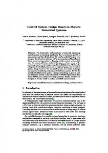
Qm = ∅ A finite state model of each of the machines M1 , M2 , M3 is illustrated in figure 1.3. The product operations of the machines M1 , M2 and M1 , M3 are shown in figure 1.4. Notice that the finite state automaton resulting of M1 × M2 in the left figure is restricted to the initial state AC since the automata have no common events, whereas in the right figure the product result evolves from the state (AE) to (BF ) due to the event (b). F IGURE 1.3: finite state model of M1, M2, M3 machines

F IGURE 1.4: Product operation of finite state model for M1, M2, M3 machines

1.2.2

Sample-driven modeling

Sample-driven models handle values, instead of events. The main difference comes from the abstraction level between these two notions. Events are considered abstract modeling artifacts, and one possible implementation of an event synchronization mechanism is the continuous sampling of a value. Sampling requires a clock, and a sampling frequency. In the sample-driven modeling there exist only one event which is a hardware clock tick. At each clock tick, all system’s inputs are sampled and their values are read and all transitions are triggered. The next state is calculated with respect to the current state and the values read from the environment. An implicit transition is modeled if no change of state is needed regarding the input sampling as shown in figure 1.5. The actual clock frequency remains abstract and remains to be subsequently determined at a physical implementation step. It is assumed, and this assumption remains to be


15

physically validated, that the clock frequency is sufficient for an accurate observation of the environment dynamics. F IGURE 1.5: Sample-driven model of a FSM

Definition 1.6 (Sample-driven finite state machine). A sample-driven model of a discrete event system can be presented as a FSM of a 4-tuple hq0 , X, δ, Q, Qm i where: • q0 is the initial state; • X is set of Boolean input variables; • Q is set of states, represented by state variables; • δ is the transition function: δ : Q × B|x| . The behavior of a discrete-event system modeled by a sample-driven finite state machine can be expressed by the algorithm [20] Algorithm 2: algorithmic description of the Sample-driven paradigm 1: initialization: i = 0, q i = q0 2: forever, at each clock tick i do 3:

read input variables xi

4:

calculate the next state: q i+1 = δ(q i , xi )

5:

update state q = q 0

6: end


Translating event-driven into sample-driven models

We use in the following the common notation for the classical Boolean operators, such as : “ ∧ ” for the logical “and”, “ ∨ ” for the logical “or”, ¬a for the logical negation of a, “→” for the logical implication and “⇔” for the Boolean equivalence. To simplify the figures we use “ . ” instead of “ ∧ ” In this work we focus on hardware systems, which are modeled using sample-driven finite state machines. However, we argue that the results presented in the sequel can also apply to eventdriven models. These can be systematically translated into sample-driven representations [23]. The transformation method we consider, between an event-driven model into a sample-driven model, is quite straightforward, and simply recalled here. Events can be translated to vectors of values, one vector per event. Thus, each event is mapped to a unique Boolean encoded value according to a function: enc : Σ → Blog2 (|Σ|)

(1.11)

Applying the encoding function enc to any event-driven FSM M E = hq0E , ΣE , δ E , QE , QE mi results in a sample-driven representation of the same machine M T = hq0T , X T , δ T , QT , QTm i, where: • QT = QE ; • q0T = QE 0; |ΣE |

• X T = xT0 xT1 ...xTn−1 where n = log2

;

• δ T : QT × Bn → QT , the transition function, which is defined as follows δ T (q T , xT ) =

  δ E (q T , enc(σ) 

q

T

if σ ∈ ΓE (q)

 

(1.12)

if σ ∈ ΣE \ ΓE (q) 

• QTm = QE m The act of sampling an event-driven model M involves a clock, which is required to be unique for the whole system, otherwise no synchronization is directly possible. It is assumed that the frequency of the clock is sufficiently high to capture the occurrence of any event from Σ. Under these assumptions of clock unicity and sufficient frequency, the clocking mechanism can be abstracted away from any sample-driven model. A physical clock signal is introduced only at a physical hardware implementation step.


17

Example 1.4. Let M = hq0 , Σ, δ, Q, Qm i be a three-states machine, where: • The initial state is q0 = A • The list of expected events is Σ = {e1 , e2 , e3 , e4 } • The set of states is Q = {A, B, C} • The set of marked states is Qm = ∅ • The transition function is δ : Q × Σ → Q where:

δ(q, (ei )) =

  (δ(A, (e1 )) = B        (δ(A, (e3 )) = C

(1.13)

  (δ(B, (e2 )) = C       (δ(C, (e4 )) = A A graphical representation of this machine is illustrated in figure 1.6 F IGURE 1.6: Sample-driven to event-driven modeling

As the machine receives |Σ| = 4 events, then, log2 (4) = 2, two Boolean variables are needed and sufficient to encode the events and translate them into Boolean input variables. Let X = {x, y}. Let enc(σ) be an encoding function computing values for the vector (x,y) and defined as: enc(e1 ) = (1, 1); enc(e2 ) = (0, 1); enc(e3 ) = (0, 0); enc(e4 ) = (1, 0) The translation of M from event-driven into a sample-driven model M T is illustrated in figure 1.6 (a) and (b) respectively. All the remaining combinations of (x) and (y) not corresponding


to e1 . . . e4 are self-loop transitions in M T , left unrepresented for more clear readability of the figure. Through application of enc−1 they would fall into the abs event labeling a supplementary self-loop transition. Notice that the inverse process of building an event-driven model from a sample-driven one through enc−1 does not necessarily yield the initial event-driven model. This happens because enc is not bijective; it is forced in that sense through the addition of the abs event, whose presence is not natural in an event-driven model.

1.2.2.2

Modeling interaction

Embedded systems are inherently concurrent systems. Concurrency is featured between building blocks, but also with the surrounding physical environment. This parallel execution requires communication abilities between the different elements, in order to establish interaction. For this purpose, the sample driven FSMs are extended with outputs. F IGURE 1.7: Environment of a block

There exist two possibilities to model outputs: (1) An implicit representation of outputs i.e, the input alphabet of an event- or sample-driven FSM is defined as a set of pairs of input/output events. This technique has been applied in [22] for modeling concurrent control systems. (2) An explicit representation of outputs i,e outputs are separated from the inputs. In our work we adopt the second choice since it is more considered a more natural modeling practice by hardware design engineers. Thus, finite state machines communicating through outputs are defined as follows: Definition 1.7. A FSM with outputs is a 6-tuple: M = hq0 , X, Q, δ, P ROP, λi where: q0 , X, Q, δ are exactly as defined above, and P ROP, λ are defined as follows: • P ROP = {p1 , ..., pk } is a set of k atomic Boolean propositions;

(1.14)


19

• λ : Q → Bk is a labeling function, modeling the outputs of M ; Depending upon how outputs are handled during modeling, two approaches exist: associate output assignments to either states or transitions. Thus, Moore-like FSMs associate outputs to states, and Mealy-like FSMs associate outputs to transitions. More specifically, in a Moore machine, the output function λ : Q → Bk is defined as: F or i = 1 to k : λi (q) = 1 iff pi is true in state (q).

(1.15)

In a Mealy machine, the output function calculates the value of an output variable for a given couple (state, input) (q, x), i.e., outputs are associated to transitions: λ : Q × B|X| → Bk is defined as F or i = 1 to k : λi (q, x) = 1 iff pi is true in state (q) and the input equals x

(1.16)

Let us define a reverse mapping λ−1 able to associate a given Boolean predicate defined on the elements of P ROP to the set of states in Q where this predicate holds. Let P represent the collection of all the possible Boolean predicates constructed with atomic propositions from P ROP . We have P ROP ⊂ P. The reverse mapping λ−1 : P → 2Q , is defined as follows: • for pi ∈ P ROP : λ−1 (p) = {q ∈ Q|λi (q) is true } • λ−1 (a ∧ b) = λ−1 (a) ∩ λ−1 (b) with a, b ∈ P; • λ−1 (a ∨ b) = λ−1 (a) ∪ λ−1 (b) with a, b ∈ P; • λ−1 (¬a) = Q \ λ−1 (a), with a ∈ P; Example 1.5. Consider the finite-state machines shown in figure 1.8. They illustrate the distinctions between Mealy/Moore modeling styles. The character ’*’ denotes any Boolean value. Both models have the same set of states: {I, W, A}, and receive the Boolean inputs {req, go, stop}, and assign the output (done). The machines are identical in behavior, they just differ in the moment of delivering the output. In the Moore machine, figure 1.8 (a) the output only depends on the system’s state. We suppose the output function definition as follows: λ(I) = {¬done}; λ(W ) = {¬done}; λ(A) = {done}.


In the Mealy machine, figure 1.8 (b), outputs are associated to transitions. To make this Mealy machine identical to the Moore one its output function should be defined as follows: λ(I, (req, go, stop)) = {¬done}, if (req, go, stop) = (∗, 0, ∗) λ(I, (req, go, stop)) = {done}, if (req, go, stop) = (1, 1, ∗) λ(W, (req, go, stop)) = {done}, if (req, go, stop) = (1, 1, 0) λ(W, (req, go, stop)) = {¬done}, if (req, go, stop) = (∗, ∗, 1) or (∗, 0, ∗) λ(A, (req, go, stop)) = {done}, if (req, go, stop) = (∗, ∗, 0) λ(A, (req, go, stop)) = {¬done}, if (req, go, stop) = (∗, ∗, 1) F IGURE 1.8: Moore vs. Mealy FSM models

1.2.3

Synchronous product with interaction

When finite state machines work concurrently and interact, a synchronous product of the two machines M1 ||M2 is calculated under the assumption that the outputs of the product are uniquely assigned by either M1 or M2 . Interacting FSMs are composed according to the synchronous paradigm defined in [21]. This operation requires a preliminary input/output mapping, usually performed by the design engineer Let Mi , i = 1, 2 be two communicating finite state machines, where Mi = hq0i , Xi , Qi , δi , P ROPi , λi i. The set of inputs Xi of Mi is divided into 2 disjoint subsets : Xi = Li ∪Ii . The machines M1 , M2 out communicate through P ropout where P ropout ⊆ P ROP1 is a subset of Boolean 1 , P rop2 1

propositions which connects M1 to M2 via L2 and P ropout ⊂ P ROP2 , is a subset which 2 connects M2 to M1 via L1 . This interconnection is illustrated in figure 1.9


21

The synchronous product M1 ||M2 is represented as: M1 ||M2 = h(q01 , q02 ), X12 , δ12 , Q12 , P ROP12 , λ12 i

(1.17)

where: • Q12 = Q1 × Q2 ; • X12 = I1 ∪ I2 ; • δ12 : Q1 × Q2 × B|X1 | × B|X2 | → Q1 × Q2 is defined as:

|L |

δ12 (q1 , q2 , i1 , i2 ) =(δ1 (q1 , i1 , λ12 (q2 ), · · · , λ2 1 (q2 )), |L |

δ2 (q2 , i2 , λ11 (q1 ), · · · , λ1 2 (q1 ))); • P ROP12 = P ROP1 ∪ P ROP2 ; • λ12 : Q12 → B|P ROP1 |+|P ROP2 | the output function is defined as: λ12 (q1 , q2 ) = (λ1 (q1 ), λ2 (q2 ))

(1.18)

Q1 ×Q2 The expression of the reverse function λ−1 is the following: 12 : P ROP1 ∪ P ROP2 → 2 −1 −1 λ−1 12 (p) = λ1 (p) × Q2 ∪ λ2 (p) × Q1 .

(1.19)

F IGURE 1.9: Product of communicating FSMs

1.2.4

Efficient manipulation of symbolic models

Binary Decision Diagrams, that we abbreviate BDDs [24] have shown their efficiency in manipulating Boolean expressions. They have been successfully used for efficient FSM representation


and state exploration [16, 25, 26]. A BDD represents a Boolean expression as a direct acyclic graph, having two terminal nodes: true (1) and false (0). Their key advantage is the ability to provide a compact and canonic representation of a Boolean expression. Thus, constructing a BDD implicitly assess the satisfiability of the Boolean expression which is represented: a tautology is always represented by the terminal node (1), and a contradiction by the terminal node (0). Besides, all Boolean operations have a corresponding efficient BDD implementation. For a given Boolean expression defined over a set of Boolean variables, building a BDD involves choosing an a priori total variable order. The key measure of BDD efficiency is the size of a BDD: the number of graph nodes required to build the diagram. The theoretical spatial complexity of a BDD is exponential in the number of Boolean variables contained. The size of a BDD strongly depends on the initially chosen variable ordering. In practice, “good” variable orders can often be found, but unfortunately there is no tractable way to compute the best variable ordering. However, BDD packages implement interesting heuristic techniques for handling variable orderings dynamically yielding fairly good performance. Besides, for some known Boolean expressions, good variable orderings simply do not exist. BDD-based formal techniques have reached their limits in terms of performance this is why most industrial and research efforts focus on the synergy between several techniques. Thus, BDDs are combined with SAT-based approaches (Satisfiability formal verification) [27] in order make the handling of large systems more tractable. Given a propositional formula ϕ, the Boolean Satisfiability problem posed on ϕ is to determine whether there exists a variable assignment under which ϕ evaluates to true in certain part of the total state space. If such assignment exists the ϕ is called satisfiable. Otherwise ϕ is said to be unsatisfiable. In this work, an important part of our results rely on the symbolic Discrete Controller Synthesis technique, with a BDD-based implementation.

1.3

Behavior requirements specification

Modeling the behavior of hardware systems is usually achieved using hardware description languages like VHDL [28] and Verilog [29] or even system-level languages such as SystemC [30]. These are standard (IEEE) languages; they are dedicated for embedded hardware modeling and can be exploited by design tools for simulation, hardware synthesis, or formal verification. However, any design process is a part of a more complex design flow, starting with requirement specifications. This process starts with functional requirements asserted informally (natural language). These requirements are first formalized, and then progressively refined, using UML or

1.3. BEHAVIOR REQUIREMENTS SPECIFICATION

23

SysML. Through such a process, a functional architecture (system-level) is refined into an organic architecture, and functional requirements are progressively mapped to behavioral requirements. These relate to the sequential behavior of a component, modeled as a communicating Boolean finite-state machine. Such requirements can be expressed formally either logically, using propositional and/or temporal logic, or operationally, by describing the desired behavior as a program.

1.3.1

Logic specifications

Logic specifications are Boolean assertions built over variable names, Boolean operations and temporal operators, expressing the relationship between the system behavior and abstract or explicit time. Such expressions extend the classical Boolean logic and are known as temporal logic formulæ, or temporal properties. Temporal logic is an important specification tool, used by embedded design engineers as a means of formalizing an expected behavior of a system [31]. Its interest is confirmed by the fact that is has become a IEEE standard [32]. Besides, a number of commercial tools [33, 34] are able to process it. The most frequently used formulædenote the following properties: • Safety: an unwanted behavior can never be observed during the system’s life cycle. Such requirements express dangerous states or input/output sequences; • Liveness: a desired behavior must eventually occur, at least once, during the system’s life cycle. It can be a state that raises the accomplishment of certain mission or the end of a functional phase; • Fairness property: this notion is close to the liveness, with a difference that the fairness requires that certain states of the system must be visited infinitely often during the system life cycle. Fairness properties are used to express repetitive behaviors either for the system or its environment. Indeed, reactive systems operate continuously hence they feature repetitive behaviors which are formalized by fairness properties. This mechanism is similar to the state marking used in event-driven modeling. Among the variety of existing temporal logics, two variants are more frequently used, essentially because they are supported by most formal tools, either academic [16, 35] or industrial [33, 34]: the Linear-time Temporal Logic and the Computation Tree Logic.


Linear-time temporal logic (LTL)

Temporal logic has been defined by Pnueli in [36]. Temporal logic uses tense operators, like “always”, “next time”, “before” and “until”, to express the evolution of a system through the time. The system’s behavior is viewed as an infinite collection of linear traces. Each trace describes an infinite sequence of states. Each state inside a trace can have only one successor. Linear-time formulæare required to hold in the initial state of the system: • Gp : p should hold forever; • F p : p should hold in some state in the future, at least once; • Xp: p should hold in the immediate next state; • p U q: p should hold until q holds, and q is required to hold eventually; • p W q : p should hold until q holds, and q is not required to hold; • p Before q: this is equivalent to ¬q W (p ∧ ¬q). This requirement states that q should never hold until p holds. If p occurs, q may occur afterwards.

1.3.1.2

Computation tree logic (CTL)

In the branching time logic, several executions are possible at a given point in time. Every state has a unique past and many future possibilities as shown in figure 1.10. CTL logic formulæcombine the Boolean logic with two path quantifiers and state quantifiers. The path quantifiers are summarized as follows: • The universal path quantifier Aϕ: means the property ϕ should hold on all the branches of the computation tree starting from the current state. • The existential path quantifier Eϕ: means the property ϕ should hold on at least one path of the computation tree starting from the current state. The state quantifiers are summarized as follows: • Next-time operator Xϕ: means that ϕ should hold in the exact next state; • Future operator F ϕ: means that ϕ should hold at least once in the future ;


25

• Global operator Gϕ: means that ϕ should hold on all the states in the future; • Until operator ϕU ψ: means that ϕ should hold until ψ holds. According to these elements, a CTL formula constructs as follows: Definition 1.8. The syntax of CTL formulæis defined as follows: • every Boolean atomic proposition is a CTL formula; • if ϕ and ψ are CTL formulæ, then ¬ϕ, ϕ · ψ, AXϕ EXϕ, A(ϕU ψ), E(ϕU ψ) are CTL formulæ. F IGURE 1.10: CTL tree logic, [1]

Branching time provides flexibility in expressing systems of complex behavior. It can express the functional behavior of a system through temporal properties: 1. Safety : AG(¬ϕ), given ϕ is a dangerous behavior of the system. As long as the property holds, the system is safe. 2. Liveness : AF (ϕ), given ϕ is a required behavior of the system that must occur at least once in the system life cycle, the system is alive as long as the property holds. 3. Faireness : AG AF ϕ, this property means (ϕ) must occur eventually often during the system life cycle. 4. Acknowledgment : AG(a → AF b), given (a) a request that needs to be acknowledged by (b). this property usually used in control systems to verify that commands have been taken in account or not.


Logical specifications have a truth value for any state of a FSM model. We write P, s |= ϕ, meaning that formula ϕ is true in state s of P . Logic specifications (LTL or CTL) are provided by most formal academic and commercial tools. However, LTL and CTL do not have the same expressive power. Most useful requirements can be expressed in both, but they also feature very subtle differences, which are quite confusing for design engineers. For example, the LTL formula F Gp can be easily confounded with the CTL formula AF AGp, saying that they are logically equivalent on a the same system, which is not true. Anyway, the “flavor” choice, linear-time or branching-time, is mainly a matter of designer’s preference. Besides, some commercial formal tools are restricted to very simple logic specifications, officially for efficiency and scalability reasons. In such situations, a possible workaround is writing operational spefications.

1.3.2

Operational specifications

Operational requirements can be specified by a “program”, modeled as one or more interacting finite state machines. Two modeling approaches co-exist in embedded design: • a reactive program, modeled by a communicating FSM featuring the required input/output mechanisms, as well as the required dynamic behavior; such a program is regarded as a “golden” or reference model, and further implementations should relate to this model, formally or not. For instance, arithmetic operations can be specified as golden models, and their hardware implementation should be proven equivalent to this model; • a reactive program equally modeled by a FSM, but whose purpose is merely observing values, and/or sequences of values, and asserting an error, by assigning a dedicated output, whenever an unwanted configuration is reached. Such a model is called an observer or a monitor [37] Example 1.6. Monitor for alternative behavior Let p be a requirement expressing alternation between two observed values (a, b). At the first cycle, a should be true, whatever the value of b, then immediately after, b should be true. This property is illustrated by the automaton shown in figure 1.11 (a). The monitor which observes this property is illustrated in figure 1.11 (b). As soon as the desired behavior does not happen any longer, the monitor switches to an error state. Monitors are usually written manually. They may be preferred to logic specifications if the requirement is easier to express operationally, such as desired sequences. It is equally possible, as shown later in this document, to transform formulæfrom a subset of the temporal logic into an equivalent monitors [38].


27

F IGURE 1.11: Alternative occurrence of events

Notice that a monitor only outputs one information: at each time moment t, it asserts whether the observed behavior has been true up to t or not. Hence, monitors can only express safety properties, and no liveness requirement can be translated into a monitor because of this lack of anticipation.

1.3.3

The Property Specification Language (PSL) standard

PSL [32] is the IEEE standard language allowing expression of behavioral requirements either as logic specifications or as operational specifications. It is a formal language developed by Accellera1 , which is an independent, non profit organization promoting modeling and verification standards for use by the electronics industry. PSL is heavily based on the proprietary language Sugar, developed by IBM and initially supported by their commercial formal verification tool RuleBase. Sugar is a syntactic layer over ordinary temporal logic, allowing shorthand expression of some common behaviors. These mechanisms were mere syntactic sugar, as they could always be translated into ordinary CTL. On the other hand, Sugar also supported operational specifications through a language heavily inspired from the CMU-SMV symbolic model checker’s input language. The CMU-SMV language can express dynamic behaviors modeled as communicating synchronous Finite State Machines. Hence, PSL contains both linear-time and branching time temporal logic, and can express requirement specifications operationally. Example 1.7. A few properties written in PSL • A Boolean expression: (start ∨ go), it means the system receives one of the two signals (start, go) or both at the instant (t); All Boolean operators can be used in PSL expression like (∧, ∨, ¬, →) 1

http://www.accelera.org


• A PSL sequential expression: (req; ack; ¬req; ¬ack); it means the signals req, ack appears in a certain sequence : req is asserted first, then ack, then req is de-asserted and then ack is de-asserted. • A PSL property can be the combination of the two expressions together using the temporal operator like (always, next, until, before, ... etc): always{start∨go}next(req; ack; ¬req; ¬ack) which means always if (start) or (go) is asserted, it will be followed by the sequence of req, ack and their de-assertion. always{request} bef ore{acknowledge} which means the signal request appears before the signal acknowledge but not necessarily in the exact previous instant. The PSL standard is currently an input for commercial (formal) verification tools and has been successfully used within academic or industrial projects [39], [40], [41].

1.4

Verification of hardware embedded systems

Hardware designs are largely modeled using Hardware Description Languages (HDL). Correct behavior of the design needs to be verified. This amounts to establishing a relationship between the design itself and a requirement. This relationship expresses satisfaction and/or confidence in the design that has been produced. It can be established either semi-formally, or formally. A semi-formal verification relies on an executable model of the design which is run for a given amount of hand-made scenarii and a given amount of time, and its outputs are inspected, more or less visually. The assessment is extremely partial, as simulation is only as exhaustive as the humans who wrote the scenarii. More recently, since PSL has emerged, requirements can be formalized. The simulation can now be run together with and against executable models of PSL specifications. This can be achieved as PSL logic specifications can be translated into monitors: • safety requirements can be directly translated into an equivalent monitor; • liveness requirements monitors can only provide an approximate assessment. They are only able to assert that a desired configuration has been observed in the past, or not. Formal verification requires a formal (mathematical) design model, and a formal specification. A translation process maps design language constructs to a formal model prior to the actual verification process.

1.4. VERIFICATION OF HARDWARE EMBEDDED SYSTEMS

29

Catching most design errors during the early phases of a design processes is vital. The next section presents a series of formal and semi-formal verification techniques which are frequently used in industrial projects.

1.4.1

Theorem proving

The theorem proving technique operates on the formal model of a design, which is handled as a set of axioms. The design needs to be translated into a set of mathematical definitions using first or higher order logic. The desired properties of the system are expressed as theorems. Theorem proving applies inference rules and induction to the system’ formal model, attempting to prove the target theorem. The advantages of the theorem proving technique are the following: • it handles efficiently the size of the design’s state space; • it handles abstract data types, and induction, which makes it a powerful tool for either finite or infinite state systems; due to these qualities, it is a particularly effective tool for assessing the correction of arithmetic components; • theorems are potentially more expressive than temporal logic. Unfortunately, theorem provers are not user-friendly tools. As they can be applied in a general framework, with possibly models featuring an infinite number of states, decidability issues can occur. Besides, the proof process needs sometimes additional guidance from the designer, which is error-prone. It may also loop forever. Some software tools have been developed to automate the process of theorem proving, in order to solve the problems in reasonable time and enhance the performance of the verification process (complexity, efficiency .. etc). The prototype verification system PVS [42], [43] is a platform supported by a specification language and verification tool based on theorem proving method. It has been successfully used to verify hardware designs [44], or a shutdown protocol of a nuclear system [45]. The Fischer’s real-time mutual exclusion protocol and a railroad crossing controller [46] were also verified using PVS. Zenon [47] is another experimental automated verifying tool, invented and dedicated for Focal environment. It provides an execution OCaml code and a Coq certification code. Isabelle/HOL [48], HOL-TestGen [49] are classical theorem provers based on the higher order logic HOL. Although automated theorem proving has solved the problem of verification time, its main drawback is the need of user assistance to guide the proof. Besides, if a theorem proof fails, it is difficult to get diagnosis/debugging information.


1.4.2

Guided simulation

The guided simulation requires the formal specification of both the design requirements and simulation scenarii. The design is run randomly together with its formally specified requirements, according to the simulation scenarii. Guided simulation is used to verify industrial systems. A bus arbiter controller was verified for mutual exclusion and conservativenes properties, using guided simulation method [50]. In [51], simulation essays were applied on the missile Titan IIIC digital flight control system in order to verify its correctness. According to the authors, the simulation scenarios were carefully chosen to cover the entire control system of the missile functionality. The author in [52], proposes a heuristic that avoids a blocking verification search by tracking multiple promising states and backing-off when getting stuck. An abstraction-guided simulation approach was proposed in [53] to combine the advantages of simulation and mathematical verification techniques, in order to find some hard to find states with a microprocessor checking. Author’s contribution was building a Markov model of the studied system and apply simulation essays on it. They demonstrate by experimental results on microprocessors, that their approach is efficient in covering hard-to-reach states, for large and complex designs. This technique can be used for medium or large sized designs, without any complexity issues. It provides acceptable coverage, and demonstrates efficiency in discovering design errors. It may however be argued that the verification is not exhaustive, and that no absolute correction guarantee can be offered.

1.4.3

Model checking

The model checking is another formal verification technique. It achieves an exhaustive exploration of the design’s state space, in order to check the satisfaction of a requirement written in temporal logic. In case the design does not satisfy the requirement model checking tools provide a counterexample that illustrates how the requirement was violated. The Model checking appeared to solve the problem of concurrent program verification, where concurrency errors are difficult to find since they do not reproduce in the program very often. At the beginning, proofs were conducted by hand using the Floyd-Hoare logic formalism. A system was proposed by Owicki and Gries [54] for reasoning about conditional critical regions. The work of Pnueli [36], Owicki and Lamport [55] proposed the use of temporal logic for specifying concurrent programs. Although they still advocated hand constructed proofs, their work demonstrated convincingly that Temporal Logic was ideal for expressing concepts like mutual

1.4. VERIFICATION OF HARDWARE EMBEDDED SYSTEMS

31

exclusion, absence of deadlock, and absence of starvation. Clarke and Emerson [56] proposed an algorithm that automatically reasons about temporal properties of finite state system by exploring the state space. K. McMillan in his PhD thesis develops the symbolic model checking technique, and the CMUSMV tool [16] to verify the satisfaction of temporal properties in a modeled system. The tool is based on Binary Decision Diagram (BDD) structure instead of stat graph and uses a special input language to represent the models and the temporal logic for the specified properties. The symbolic method coupled to BDDs has shown outstanding performance figures, and most commercial formal verification tools exploit this principle. Bounded model checking was introduced in 1999 [57] by A. Biere et al. The core of this strategy is to verify the satisfaction of a property of a system under fixed number of steps (k); one keeps increasing (k) as long as the property is satisfied and stops when the property is violated or when decide that k is enough to decide the satisfiability of the property. This method uses the state graph as data structure and can be applied to both safety and liveness properties, but it suffers from being always bounded, so one cannot validate a studied system except for limited number of states. Edmund M. Clarke in [58] explains some advantages of model checking, we cite here some of them: • fully automatic method: the user of a Model Checker does not need to construct a correctness proof. In principle, all that is necessary is for the user to enter a description of the circuit or program to be verified and the specification to be checked. The checking process is fully automatic; • rigorous: when a specified property is not satisfied by the model studied, the model checker provides a counterexample illustrates where the property was violated, and this is one of the most important features of using model checking technique; • powerful: employing temporal logic allows to consciously expressing complex properties, and it helps to reasoning concurrent systems while it is very hard to verify all possible cases manually. Unfortunately, a serious problem of which all the model checkers suffer is combinational explosion. A system with n Boolean state variables has 2n possible states. This blow-up happens during BDD construction/manipulation. Even though BDDs allow efficient manipulation of large sets of states, their theoretic complexity is still exponential in the number of Boolean variables handled. Thus it is sometimes impossible to explore the entire state space with limited resources of time and memory [59].

32CHAPTER 1. SAFE DESIGN OF HARDWARE EMBEDDED SYSTEMS BASED ON COTS : STATE OF THE ART TABLE 1.1: comparison between different formal verification techniques

state space coverage free software counterexample fully automatic verification large state space concurrency

Theorem proving + + + +

Guided simulation + + +

Model checking + + + + +

Industrial and research efforts have concentrated on these performance issues. SAT-based techniques [60] have been developed, featuring considerable performance, and requiring much less memory. Nowadays commercial tools are able to combine several state traversal techniques, switching dynamically from one to the other. Hence, random guided exploration can narrow down the state space, getting “closer to the final solution”; then, an exhaustive BDD-based exploration can start, implemented by a parallel algorithm. Thus, model checking is still an important design tool which is able to uncover corner-case subtle design errors [61]. The following table illustrates a comparison between the theorem proving, guided simulation and model checking regarding some key features : Regarding the 1.1 table we suggest in our contribution to use the model checking technique and take advantage of its features (fully automatic, full coverage of state space, counterexample providing, accept symbolic representation of a system), to find the design errors and rigorously get a trace when a property is violated by the original system specification.

1.5 1.5.1

Supervisor synthesis Supervisory control

This work advocates the use of the supervisory control theory - also known as Ramadge and Wonham framework [62] - as a complementary embedded design tool. This theory has been developed on top of formal languages, more particularly the regular languages. Just like formal verification, this theory applies to finite state/transition models, directly derived from regular languages. Unlike verification, rather then checking whether a system satisfies a formally specified requirement, this control paradigm enforces requirements, when possible. To achieve this, a supervisor is automatically generated from the design at hand, also known as the plant, and the formally specified requirement. The supervisor acts as a new building block, running concurrently with the plant, and communicating with it: reading state information from the system and the environment, and feeding control information back to the system, in order to enforce

1.5. SUPERVISOR SYNTHESIS

33

the desired requirements. Thus, a “closed-loop” control architecture is provided. Typically, a desired behavior is made either invariant (safety), or reachable. It is also possible to enforce unavoidability (liveness) in an approximate way, by solving this problem as an optimal path problem, such as proposed in [63]. In this work, safety is the only requirement that is considered. This limitation is mainly proposed in order to simplify the application of DCS to COTS-based designs. Extensions to reachability/liveness requirements are left as future developments. The actual technique which performs the construction of a supervisor is called Discrete Controller Synthesis (DCS). In this work, safety is the only requirement that is considered. This limitation is mainly proposed in order to simplify the application of DCS to COTS-based designs. The term “controller” either designates the supervisor, or a building block obtained from the supervisor. In this work, DCS refers to both the supervisor generation and the controller construction. This aspect is developed later in this chapter. Two DCS variants exist according to the formal models upon which they have been built: event or sample-driven. Thus, the plant is either specified as a formal regular language, using exclusively states, events and transitions, or as a reactive program featuring inputs, outputs, state variables and some algorithmic structures implementing transition functions. The event-driven DCS technique initially developed by Ramadge and Wonham [62] has been recently ported to symbolic BDD-based state traversal algorithms [64], [65]. The current work is based on sample-driven models, which is why the DCS technique used in the sequel is the one developed in [66].

1.5.2

Controllability in hardware systems

Prior to recalling the DCS basics, needed in the remaining of this work, it is important to clarify some terminology elements. The DCS control design technique is used in a hardware design context and hence, some keywords common to both automatic control design and hardware design become ambiguous. Even though they are conceptually close, they do not have the same significance. In electronic hardware design, two types of building blocks are handled: (1) the controller and (2) the datapath, also known as the operative part. A datapath is a building block featuring a sequential dynamic behavior, typically arithmetic computations. The controller acts as a scheduler for the different arithmetic operations that are needed in order to implement a requirement. Hence, both the controller and the datapath are modeled using the same language, have the same underlying formal model, and most often are implemented in the same electronic chip.


The high-level synthesis [67] technique achieves automatic generation of both the controller and the datapath, according to a user-defined specification issued as an iterative algorithm. This context is close to the supervisory control theory. Two types of interactions exist: with the physical environment, through uncontrollable inputs (or events), and with the operative part, through controllable inputs, which are seen as actions taken by the controller. The conceptual distinction between these two kinds of inputs is obvious, and the partitioning too. However, this case remains an exception. Many hardware designs do not feature a clear frontier between the control and operative parts. Besides, control functions are often complex operations, featuring concurrent behaviors. They are manually coded by design engineers, and due to their complexity this process is error-prone. In this work, such control functions are considered as candidates to control, in order to enforce a requirement. Unfortunately in this context, is is much more difficult to partition the input interface of a building block with respect to controlability. This distinction is unnatural for hardware design engineers: all available input variables are considered to be driven by the environment, and the design process does not anticipate the presence of a supervisor. However, in order to apply DCS, the input variable set needs to be partitioned into controllable and uncontrollable inputs, so that the control architecture presented in figure 1.12 can be used: X = Xuc ∪ Xc . A method for achieving this partitioning is provided in Chapter 3. F IGURE 1.12: Control architecture for hardware designs

1.5.3

Symbolic supervisor synthesis

The symbolic discrete controller synthesis method was first developed in [25] [66, 68]. The symbolic DCS algorithm makes invariant the set λ−1 (spec) of states, satisfying the desired specification spec. To achieve this, it iteratevely prunes all the states from which an execution path can lead outside λ−1 (spec) through uncontrollable input values. The result of this process is a set of states, called invariant under control IUC. The calculation of the invariant under control iteratively calls a basic step: finding the list of controllable predecessors of a given set of states. This list can be obtained as follows. Given a Boolean finite state machine M = hs0 , X, S, δ, P ROP, λi, and a set E ⊂ B|S| , the set of controllable predecessors of E is defined as:


35

CP RED(E, δ) = {s ∈ B|S| | ∀xu ∈ B|Xuc | , ∃xc ∈ B|Xc | , ∃s0 ∈ B|S| : s0 = δ(s, xuc , xc , s) ∧ s0 ∈ E} In other words, the state s is a controllable predecessor of a state s0 ∈ E iff for any uncontrollable value xuc , there exist a controllable value xc such that the transition function δ leads to s0 . Hence, it is always possible to go from state s to state s0 by computing an adequate value for xc , according to s and xuc . The DCS algorithm consists of a recursive application of CP RED till a greatest fixed point is reached:

IUC 0 =λ−1 (spec) IUC k+1 =IUC k ∩ CP RED(IUC k , δ) The greatest fixed point reached is the invariant under control IUC set. A control solution exists if this result is not the empty set. Besides, the initial state of the system must be included in the invariant under control IUC. Under these conditions, the supervisor SU P is constructed from IUC as follows: SU P = {(s, xuc , xc ) ∈ B|S| × B|Xuc | × B|Xc | | ∃s0 s.t. s0 = δ(s, xuc , xc ) ∧ s0 ∈ IUC} SU P is the set of all transitions of M leading to IUC. F IGURE 1.13: A 5-states design to be controlled using DCS


Example 1.8. We consider the state-based design illustrated in the figure 1.13. Let spec = G¬(E1 ∨ E2 ) be the requirement which should be enforced on this model. Starting from the initial state A, the property can be broken in state B, uppon receiving the input req = 0. Supposing that go is a controllable variable, and req, stop are uncontrollable variables, there exist a winning strategy which assigns the value 1 to the variable go at the state A. Any other controllable variables are not enough to prevent the system from reaching the inadmissible state. By applying the computation algorithm of IUC we obtain : IUC 0 ={A, B, C} IUC 1 ={A, C} IUC 2 ={A, C} IUC 2 =IUC 1 ; A fixed point is reached and the final IUC set is {A, C}.

1.5.4

DCS for hardware designs

The supervisor provided by the symbolic DCS is a characteristic function: SUP : B|S| × B|Xuc | × B|Xc | → B defined as: SUP(s, xuc , xc ) = 1 iff (s, xuc , xc ) ∈ SU P The actual control of M requires solving the equation

SUP(s, xuc , xc ) = 1 continuously, for each reaction of M , and considering Xc as unknown variables. This is not directly implementable into hardware. We use the supervisor decomposition technique presented in [69] in order to obtain systematically the control architecture presented in Figure 1.12. According to this decomposition technique, the characteristic equation representing the supervisor SUP is automatically decomposed into a vector Cˆ of m Boolean functions, where m is the number of controllable variables.


37

f1 (s, xuc , xenv c1 , f2 , . . . , fm )



  f2 (s, xuc , xenv c2 , f3 , . . . , fm ) Cˆ =   ......  fm (s, xuc , xenv cm )

    



The variables xenv hold the values that the environment “proposes” for the controllable variables c xc . It is up to the controller Cˆ to decide whether the environment proposal is accepted or not. In the sequel, the decomposed supervisor Cˆ is referred to as the controller. Example 1.9. The supervisor decomposition for the previous example yields a controller containing one function which assigns values to the controllable input go:

go = f (s, req, goenv ) where the expression of f is :

f (s, req, goenv ) = if (s = A) ∧ (req = 1) then go := 1 else go := goenv

Thus, if state A is active and the req input is asserted then go is assigned to 1. Otherwise, go receives the value goenv assigned by the environment. The resulting controlled design is shown in Figure 1.14. F IGURE 1.14: A 5-states design assembled to the controller

Hence, the dynamics of the controlled design is presented by the following algorithm:


Algorithm 3: sample-driven execution of a controlled design 1: initialization: i = 0, q i = q0 2: for each clock tick i do 3: sample all uncontrollable variables xuc and all desired controllable values xenv c env ˆ 3: compute the controlled values xc = C(s, xuc , xc ) 4: compute the next state: si+1 = δ(si , xuc , xc ) 5: compute the outputs: oi = λ(si , xuc , xc ) 6: end for According to the dynamics described above, at each reaction, controllable inputs xc are driven by the environment and controlled (modified) by the supervisor, according to the current state of the design and the satisfaction of the control specification. Both M and the decomposed supervisor can be directly implemented on hardware targets. A concrete example is developed in Chapter 3 of this document.

1.6

COTS-based design

The term COTS is an abbreviation standing for Commercial Off The Shelf. A COTS is a generic, reusable, hardware or software component. Although, there is no component that can do everything and can work everywhere, COTS developers provide components with generic behavior, which can be used for different applications. A component is considered reusable COTS when it satisfies certain functional requirements when integrated in certain environments. The main advantage of using COTS in a design, is to economize time and production costs [70], and also to provide fault tolerance in circuits [71]. The companies use in-house COTS, fabricated by the company itself or out-house COTS, also called IP2 components, that it buys from the existing market. Big industrial companies like military, avionic, transport companies, can also solicit smaller companies to fabricate special COTS suitable with their own interests and needs, especially if they do not own a development staff to do this mission.

1.6.1

COTS definitions

In the last decades, several definitions of COTS were given, starting from very general notion of re-usability going to a more precised characterization of reusable components. In 1997, [72], a COTS was defined as a black box, where no access to its behavior is available, nor fully access to its documentation is possible. In 1998 [73], COTS was considered as any pre-built 2

Intellectual property

1.6. COTS-BASED DESIGN

39

component, available for the public, which can be bought, leased or licensed, and integrated in a larger system in order to achieve certain mission. The federal acquisition regulation (FAR), in part 12, defines the commercial item as follows "An item is sold, leased, or licensed to the general public; offered by a vendor trying to profit from it; supported and evolved by the vendor who retains the intellectual property rights; available in multiple, identical copies; and used without modification of the internals." [74]. In 2002 [75], seven attributes were considered necessary to any component to be considered COTS, the attributes put frontiers to the vague definitions of COTS. (1) A COTS is generally a purchased component. (2) a license must be given to the customer. (3) the possible modification could be applied to the COTS are limited to parameterization. (4) the COTS should be stocked in a library. (5) medium size component. (6) the component must have an interface. (7) it must have vertical functionality, i.e; it must be used in many applications. A formal definition of COTS will be presented latter in this manuscript.

1.6.2

COTS integration in a design process, difficulties and solutions

The lack of formal specification of pre-built components behavior was an obstacle against using COTS in critical systems, thus, a formal definition of COTS interface was proposed in 1999 [76]. Formalizing contracts over the COTS interface isolates the system under construction of the COTS internal software and makes the interaction between the original system and the integrated COTS verified and controlled through the interface contracts. In 2005 A formal definition of Component-based embedded system was proposed in [2]. A communication level specification of components, based on extended finite state machines (EFSM), was used. The studied embedded system is divided into three sorts of communicating blocks (1) sensors, (2) a controller and (3) actuators as shown in figure 1.15. Components are connected by communication points, i.e., inputs and outputs. sensor’s outputs are input events for the controller, the controller’s outputs are the inputs of the actuators. The system components are black boxes specified and tested using formal description technique, Estelle [77], [78]. The specification approach reuses an already existing methods to formally define embedded systems and profits of methods like automatic analysis, test data generation, validation and formal fault models, to enhance the components based development and follow the growing complexity of embedded system requirements especially safety and real-time properties. Using COTS in a design, although it facilitates the cost of initializing a system design, it raises the risk of component maintenance, since the original developer may not be available for checking the components. If the vendor is not capable to keep up with the customer problems or product bugs, or even the shop is closed or stopped producing such COTS, negative consequences will affect the customer design and extra unexpected expenses will be needed for any system

40CHAPTER 1. SAFE DESIGN OF HARDWARE EMBEDDED SYSTEMS BASED ON COTS : STATE OF THE ART F IGURE 1.15: Composition environment of embedded systems based on EFSMs [2]

upgrading. Thus, maintenance costs increases exponentially when integrating COTS inside the design, [79]. Thus, researchers worked to provide some heuristics in order to balance between the use of COTS in a design and the negative consequences of such use [79], [80].

1.6.3

Safety preserving formal COTS composition

Formal representation of components’ composition has been evoked in the literature of software engineering of embedded systems. In [81], [82] a formal method for developing trustworthy real-time reactive systems is proposed. The system components are a set of communicating tasks modeled as communication finite state machines, and the system’s trustworthy is evaluated by the system’s preservation of some formal safety and security properties. The model checking is used to verify these properties over the studied system. In [83] software components are modeled as communicating finite state machines and the safe communications are represented by LTL assertions. Informal lexical compatibility study is made over the components to conclude the system’s safety represented by compatible components. In [84] a monitoring data flow service is proposed to supervise the communication between some tasks modeled as FSMs. The system is composed by a synchronous product of the tasks FSMs, and the service can detect any unexpected communication over the system and signalize it as an error. Monitors are automatically generated using a particular tool named (Enforcer).

1.6.4

Safety in component-based development

In [85], safe COTS is defined as "a COTS which poses no threat or only a reduced threat in accordance with the nature of its use and which is acceptable in view of maintaining a high level of protection for the health and safety of persons".


41

In 1999, PORE (Procurement-Oriented Requirements Engineering) [3], a guiding coherent technique for component-based requirements engineering was proposed. it provides the designing team with instructions to choose COTS components. It focuses on (1) the collection of the maximum information and requirements of the system under designing. (2) the selection of various candidate COTS exist in the market. Then (3) mapping the system requirements to the selected COTS to evaluate the components candidates. and finally (4) rejecting the components that satisfies the requirements the least, and keeping the components which are the best candidates to be used in the system design, as illustrated in figure 1.16. F IGURE 1.16: High-level generic processes for PORE method [3]

The process of COTS evaluation is iterative one, i.e, requirements acquisition enables product selection and product selection informs requirements acquisition. As the number and detail of requirements increases, the number of candidate products decreases, as shown in figure 1.17 F IGURE 1.17: Overview of the PORE’s iterative process [3]

In 2003, a component based development method [86] was proposed. Basing on analytic study of the efficiency of using COTS in system’s development and the obstacles faced by such choice, the CARE method, shown in figure 1.18, comes up with evaluation, verification and validation steps, over the hardware and software parts, of the target system. The method contains eight


successive steps. It starts by a Hazard analysis and risk assessment on the conceptual system, in order to delineate hazards uncovered by the analysis. The second step is a Safety requirements specification, in this step safety verification is performed to ensure that system’s specification reflects the safety requirements. The third step of the method is safety requirements allocation, in this step safety requirements are allocated to hardware and software system’s parts. In step four, Software requirements specification, the software requirement specification is examined to ensure its inclusion of all safety requirements dictated by the former step. At step five, Software verification, a verification is performed at each phase of software development to ensure that the safety requirements are respected by the system specification. At the sixth step, Software safety validation, the software part of the system is validated if the verification step successfully passed and the safety requirements were fulfilled. In step seven, Hardware and software integration, both system parts are integrated and a verification is performed to ensure that the hardware part of the system which depends on the software part correctly operates. The eighth step, Systems safety validation, gives a final validation and assurance that the designed system is verified to fulfill the safety requirements specified for it and the system is ready to be used or supplied to the market. F IGURE 1.18: System safety V and V for COTS based systems


43

In 2004 a COTS aware requirements engineering technique, CARE [4], inspired by the PORE method was introduced. The proposal directs the designer to bridge between the native system and the requirements added by the foreign components. It raises some issues about the optimization of COTS using, like (1) determining the requirements which satisfies the final client. (2) matching the client requirements to the COTS capabilities. (3) selecting the best COTS candidate if different components exist in the market. (4) deciding whether building a system over COTS component is efficient or it is worthy to construct the system components from scratch. (5) studying the impact of COTS integration over the global system. In 2007, a formal method, MiHOS [87] [5],[88], to evaluate the matching between a system requirements and COTS product was proposed. The goal of the method is to provide the best COTS candidates to a design. The method starts by analyzing strategic goals until reaching technical requirements. The strategic goals are the global behavior required by the final system, which cannot be performed by a single component ex. a secure communication between services. The technical requirement, is a COTS technical attribute which can achieve the strategic requirement, ex. supporting SSL communication protocol. The method depends on giving weights to the system requirements and evaluating which are the COTS that match the most these requirements. The method suggests five levels of matching, "(1) Zero match, when the COTS product fails to satisfy the requirements. (2) partial match, indicates partial satisfaction of requirements. (3) surplus, indicates that the COTS has extra functionality, not needed in the design. (4) overmatch, which indicates that the COTS functionality exhibits more capabilities than required. (5) equivalence which means, the COTS contribute to achieve the goal of the requirement, but it does not match the technical requirement itself." A hierarchical definition of a COTS evaluation with MiHOS method is illustrated in figure 1.19. F IGURE 1.19: Hierarchical definition for COTS evaluation criteria [5]

A notion of trustworthy assembly of COTS is proposed in [89]. COTS were considered as black boxes and propose to solicit the UML method to represent the studied components; The work proposes to use the composite structure diagrams in order to express the architecture of components and their interfaces. They use the class diagrams, sequence diagrams and protocol state machines to describe the behavior of each component. The problem discussed is the interoperability of COTS through their interfaces. When assembling COTS, compatible interfaces are


needed, and since the COTS may be built in different companies, they probably do not share the same syntax languages, a mediator is necessary to organize the exchanges between assembled COTS. Trustworthy by verification, of hardware and software COTS based systems, was proposed in [90], where the model checking method is used to verifying if the satisfaction of some formal properties. The method validates a trusted system, if abstract models expressed in xUML or Verilog, of the real components satisfy properties written in a unified property specification language developed specially for the proposed method. From a safety point of view, the above mentioned methods are quite robust, but, some points are missed. (1) The methods do not tackle the cases where the safety norms are not respected. (2) They do not suggest implementation tools. (3) They are manual tools and strongly depend on the designer competence in requirement engineering. (4) The last trust worthy method [90] is limited in application because it necessities a designer who masters well its language of property specification, otherwise, the model checking results cannot be trusted. In our work, we fill those gaps by providing a complete method for safe design based on COTS. Our method is not an extension of the above ones, but, they are conceptually comparable to each other, as they both concern the safety of system based on COTS.

1.7

Conclusion

In this chapter we have presented an introduction about the hardware embedded systems, then the two modeling methods of the discrete behavior of these systems (event-driven and Sample-driven modeling). We have shown that the event-driven modeling is an abstract method and the Sample-driven modeling is more suitable to represent the hardware circuits, since it is closer to its material nature. We have mentioned also some assisting design method which help the designer verify his design before implementing it like: (1) the theorem proving technique, since it is manual method, it depends strongly about the experience of the verifier and its mathematical competences. It is convenient for verifying systems of certain sizes. The ATP, as it does not provide a counterexample, it is useful only to confirm that the studied specification does not satisfy the studied property. No further benefits can be reached of this method. (2) the guided simulation is suitable method for verifying certain precise behavior in an industrial large design, but, it cannot provide a complete results about the full comportment of the studied system. (3) the model checking, is much useful for verifying medium to large systems, since it is fully automatic tool, its results are trusted, as long as it does not explode. When it provides a counterexample it may inspire the designer where he needs to correct the error. All those formal verification methods, whether

1.7. CONCLUSION

45

manual or automatic are limited to only finding design errors. No matter what technique the designer used, he is still obliged to correct the detected errors manually. We have illustrated the discrete controller synthesis method, and its capability to synthesize certain behavior to discrete event systems. This method is still used only in the research domain, and we propose to integrate it in the application domain, take advantage of its services and figure out its shortcomings. We have approached the evolution of the COTS notion through time, then the safety principles in using COTS components in system designs. The safety studied focuses basically on the matching of the components selected and the existing system, it depends on analytic studies of the system requirements and the components’ behavior. If the matching is satisfied the COTS is taken for the design, otherwise it is rejected and another COTS is searched. In our work we advocate the possibility of automatically correcting mismatching COTS, through correct by construction code generation. The following chapter presents a safe COTS-based design method for hardware embedded systems.


Chapter 2

The COTS-based design method 2.1

Introduction

The former chapter provides an overview of the state of the art in the domain of designing critical hardware systems; (1) modeling the behavior of hardware systems, (2) the formal verification of hardware systems and and its utility in finding design errors (3) the discrete synthesis tool and its capacity to automatically generating a correcting component named controller which once combined to the original system, it makes the resulting assembly satisfy safety properties, (4) the COTS-based design of embedded systems and the safety notion in COTS-based systems. This chapter presents a novel COTS-based safe design method. Its novelty comes from the synergy between the formal verification and the Discrete Controller Synthesis techniques for building correct COTS-based designs. While formal verification is a mature technique in industry, DCS has never been previously in an industrial hardware design project. Besides the specific methodological aspects related to COTS design, the key issues in applying DCS to hardware designs are explained and solved. The COTS components considered here are described by a behavioral model built by their original designer. The actual user has no knowledge about their implementation details, as sometimes the design code provided is not even readable. The user side perception of a COTS is a documented black box. The requirement specifications are formally expressed PSL language. These formal specifications are either given by the COTS provider, or built a posteriori by the COTS user, from the textual documentation. The method proposed here encompasses all stages, from the initial specification to the target implementation prior to hardware synthesis. It is illustrated through a non-trivial yet pedagogic example: the generalized buffer system abbreviated as GenBuf [91]. 47

48

CHAPTER 2. THE COTS-BASED DESIGN METHOD

The rest of the chapter is organized as follows : section 2.2, defines the notion of COTS, as used throughout this work. Basic reasoning steps in COTS-based design are presented in section 2.3, followed by the articulation with the Discrete Controller Synthesis technique. DCS application to hardware designs needs a user-specified partition of the input signals set, in order to designate controllable inputs. As explained previously, this step is unnatural to hardware design engineers. A technique is developed in order to determine a set of candidates to controlability, automatically providing designers with a set of controllable candidates. These elements are aggregated within a global design method. Section 2.4 presents the example of a COTS-based hardware design. The application of the method developed here is illustrated on this example. We have presented this work in [92], [93]

2.2 2.2.1

Building COTS-based control-command systems Stand-alone COTS

In this work, the notion of COTS is mainly related to reusability. This means that a COTS is a mature building block, implementing a non-trivial behavior, for which a certain amount of design and verification efforts have been spent. This is why a COTS is not only a component having a behavior, but is also documented: this documentation states both how the COTS should be used, and what it achieves. In practice, these elements are provided informally, as text. Even though this approach is familiar to design engineers, we highlight the need for formalizing them and associating them to the COTS behavior. Building new complex functions out of COTS calls for formal tools in order to achieve a safe design. COTS are usually structured into libraries, when developed and reused by the same team. A stand-alone control-command COTS is the basic building block considered in this work. It is characterized conventionally by four elements [94] : 1. COTS interface I 2. a set of preconditions A 3. a set of post-conditions G 4. COTS functional behavior M . The set of post-conditions are satisfied by the COTS behavior if and only if

2.2. BUILDING COTS-BASED CONTROL-COMMAND SYSTEMS

49

A stand-alone COTS is atomic: no structural decomposition into other elementary COTS is possible. The COTS interface designates its set of inputs and output variables. The COTS preconditions A is a set of requirements expressed on the COTS’ environment.

The need for environment assumptions.

COTS are logical building blocks which are intended

to be assembled in order to build the final control-command system driving an operative part, as shown in figure 2.1. Hence, the environment of a COTS is rarely physical, but most often logical, made of other COTS. Complex interactions may occur between COTS through communication. In order to handle this complexity within a design team where COTS components can be developed separately, a contract-based approach is generally used [95]. Consider the COTS C and C 0 , developed separately by two designers. They each implement a specific function, and they interact with each other through inputs and outputs. At the moment of designing C, the designer reasons as follows: the design at hand assign outputs according to the values of the inputs and possibly an internal state. It often happens that some (sequences of) inputs only make sense in some given configurations. There are three possible choices: • an input value is unexpected. It should be processed and this should result in an error code; • an input value or sequence comes at the wrong moment. Either answer with an error code, or memorize it till it can be processed. Either possibilities require adding additional, often very complex code, making sure that inputs are just as expected. Testing every possible situation is time-costly and error-prone. • assume that the input values cannot be erroneous. Document this assumption. The designer of C 0 follows the same reasoning. Hence, either both designers should add extra heavy code for testing the validity of the inputs, or they both assume that invalid inputs cannot occur. This is also known as “assume-guarantee” reasoning: when designing C, it is assumed that C 0 behaves correctly. The designer of C 0 should guarantee this correction. This approach is very cost effective even though this reasoning is not always valid: typically, if the correction of C depends on the correction of C 0 and vice-versa, the assume-guarantee reasoning cannot be applied. This issue is illustrated later in this document. This work mainly addresses designs made of interconnected COTS, which is why the method we propose needs to reason about the environment behavior of a given COTS (or COTS assembly).

50

CHAPTER 2. THE COTS-BASED DESIGN METHOD F IGURE 2.1: COTS-based control command system made of interacting blocks Control/command block

commands

C Operative part

C 00 C0

sensors

The construction of the functional behavior formal model M is not mentioned in this document, as it is generally systematically and automatically extracted from the design code (VHDL or other). This is why, by an abuse of language, pieces of code are referred to as models. F IGURE 2.2: Interface of a COTS represented by X c , Y c

Definition 2.1 (Stand-alone COTS). We define a stand-alone COTS component C as a 4-tuple : C = (I c , M c , Ac , Gc )

(2.1)

We denote X c the list of COTS’ inputs, X c = {xc1 , xc2 , ... xcn }. Y c the list of COTS outputs, c }. Thus, the component interface is : Y c = {y1c , y2c , ... ym

Ic = Xc ∪ Y c

(2.2)

as shown in figure 2.2. The COTS preconditions Ac describe the expected behavior of the environment of C. They are expressed logically and/or operationally.

C Ac = {ΦC a , Ma }

(2.3)

where C • ΦC a is a set of logical specifications written in PSL, upon variables of I ;

• MC a is a set of operational specifications. They can be either monitors, expressed over variables of I C , or random FSM models, reading Y C and specifying desired values for XC.


51

The COTS post-conditions Gc is a similar set of formally specified assertions: C Gc = {ΦC g , Mg }

(2.4)

C where ΦC g is a set of PSL formulæand Mg is a set of operational specifications. The post-

condition set expresses behaviors guaranteed to hold on C, provided that the assumptions hold. The COTS’s behavior, given with the COTS documentation, is modeled by a finite state machine: M C = hs0 , X, S, δ, P ROP, λB i, where: • X = X c; • P ROP = Y c ; • s0 , S, δ, λB are defined exactly as in Chapter 1.

The COTS behavioral model is usually automatically extracted from the design code as mentioned before. The relationship between AC , GC and M C is expressed as follows: C C M C , haC 1 . . . ak i |= g

(2.5)

C The FSM model M C satisfies the requirement g C provided that all the assumptions aC 1 . . . ak ∈

AC are satisfied by the environment of M C . This dependency |= between assumptions and guarantees does not necessarily mean a logical implication. It happens that hardware designers express environment assumptions either as sufficient conditions or as necessary conditions, or sometimes both. Most often, they are perceived as necessary conditions. The difficulty of distinguishing between these two situations comes from the sequential complexity of the COTS’ behavior. It would be theoretically very interesting to automatically “extract” the set of necessary environment assumptions a COTS needs in order to operate correctly; however, such an operation is not possible to the best of our knowledge. The satisfaction relation |= has the following signification: • if g C is a logical specification, then the satisfaction is established by model checking M C C against g C by assuming aC 1 . . . ak ;

• if g C is an operational specification, then there are two possibilities:

52


– g C is a monitor. It has the form (I, MgC , ∅, φErr ), where Err is the single output of MgC and asserted true if the behavior observed by MgC violates the desired requirement. The predicate φErr is of the form “always (¬Err)”. In this case, M C ||MgC is model checked against φErr ; – g C is a “golden” , or reference FSM model. M C should be sequentially equivalent to g C . In other words, M C should have exactly the same behavior as g C . This can also be established formally, by model checking. It is important to note that the sets AC and GC contain two kinds of requirements: those expressed by the designers, which are considered as the most important, but also, in a large number, those left implicit; their exhaustive expression is both practically impossible and useless. However, some assumptions and/or guarantees which have been left implicit can simply characterize design errors, left uncovered. Indeed, uncovering a bug requires asking the “right question”, and translate it logically or operationally. This totally depends on the verification engineer’s skill, and thus, the chances of success are random. Hence, a COTS is not a “perfect” component; it can (and probably) have hidden bugs, and building designs out of existing COTS elements also amounts to mixing unwanted behaviors from each building block. In the context of this work, COTS behaviors are usually specified using the VHDL hardware description language. For the specific needs of the Ferrocots project, the ControlBuild [96], [97] graphical design environment has been used, as it provides designers with a more userfriendly design framework. ControlBuild models are assumed, without loss of generality, to have a synchronous semantics, compliant to the models defined in Chapter 1 of this document. Moreover, all ControlBuild designs are translatable into synchronous VHDL, compliant with the IEEE standard “RTL synthesis subset level 1” [98]. This compliance provides an informal guarantee that a synchronous FSM semantics can be associated to any ControlBuild design. Example 2.1. Preconditions of a stand-alone COTS Let C be a component with the set X c = {xc1 , xc2 }, Y c = {y1c , y2c }. The COTS inputs work in mutual exclusion mechanism and the environment change at each instant. The inputs are represented by an interface preconditions set Ac = {ac1 , ac2 } where: (ac1 : xc1 6= xc2 ), and (ac2 : xc1 at the instant (t) = ¬xc1 at the instant (t − 1)). In PSL these preconditions can be written as: • ac1 = always ((xc1 ∧ ¬xc2 ) ∨ (¬xc1 ∧ xc2 )) • ac2 = always( (xc1 → X(¬xc1 )) ∧ (¬xc1 → X(xc1 ))) ac1 , ac2 are illustrated by the truth table 2.1.


53

TABLE 2.1: Truth table illustrating the preconditions of a dynamic environment with a mutual exclusion behavior

xc1 0 0 1 1

next xc1 0 1 0 1

not next xc1 1 0 1 0

xc1 → not next xc1 1 1 1 0

xc1 0 0 1 1

¬xc1 1 1 0 0

next xc1 0 1 0 1

¬xc1 → next xc1 0 1 1 1

ac2 0 1 1 0

xc2 0 1 0 1

ac1 0 1 1 0

Example 2.2. Post-conditions of a stand-alone COTS Let (C) be a component with the set X c = {xc1 , xc2 }, Y c = {y1c , y2c } with a precondition list Ac = {ac1 : xc1 6= xc2 }, a post condition that must be satisfied is Gc = {g1c : y1c = y2c }. These pre/post-conditions can be expressed in PSL as follows : • ac1 = always ((xc1 ∧ ¬xc2 ) ∨ (¬xc1 ∧ xc2 )) • g1c = always (y1c ∧ y2c ) Some COTS have a combinational behavior, i.e, the outputs of the COTS depend only on the values of its inputs, As shown in figure 2.3 (a). Other components have a sequential behavior, i.e, the output of the COTS depends on the its internal state and the current values of inputs. This is shown in figure 2.3 (b). F IGURE 2.3: COTS behavior

2.2.2

COTS assembly

A COTS assembly is the act of combining components together, in order to produce a new behavior, which cannot be produced by any COTS, considered alone. The approach for assembling COTS proposed in this document relies on a rather classical conception of the component-based design: components have a behavior, a set of guarantees and and a set of assumptions, also known sometimes as contracts. The guarantees hold provided that their corresponding contracts

54


are fulfilled. The act of composing two components amounts to finding a matching between the guarantees of one component and the contracts of the other. An interaction is thus established, and some other guarantees may find themselves satisfied by simple component composition. These mechanisms are quite classical in software programming. This design approach is quite natural, and has proven its robustness. Most recent developments we are aware of, conducted within the AFSEC1 research community, define contracts for reactive timed models [99] and the corresponding compositional reasoning with contracts. Other relevant contributions close to our work have been presented in 1.6.3; they are related to software COTS-based design, where COTS are communicating tasks, modeled by finite state machines and composed together by a synchronous product. The correctness of a COTS-based design is established by model checking. In this work, we extend the classical component-based reasoning mechanisms, by identifying specific issues, characteristic for the component-based design of hardware embedded systems. We solve these issues both technically, by establishing a synergy between the formal verification and DCS techniques, and methodologically, by proposing a safe design method. When assembling hardware COTSs, the assembly interface becomes a partial part of all the interfaces of assembled COTS, some input and output signals of a COTS become internal signals. We denote (X intern , Y intern ) for internal inputs and internal outputs respectively. We denote I intern to the union X intern ∪ Y intern . Prior to achieving a COTS assembly, two kinds of functional behaviors related to either standalone COTS or COTS assemblies need to be distinguished: • the post-conditions, or guarantees, denoted by the letter G, which are originally satisfied by the COTS and cited in its documentation; • the required properties, denoted by the letter P , which are user-specified, according to the specific use of an instantiated COTS, or COTS assembly. Their validity remains to be established.

Structural assessment of COTS interconnections.

The act of interconnecting COTS relies on

a one-to-one conceptual pattern. No matter how complex the target function to be achieved, designers usually consider COTS to be assembled in pairs. Several compositional architectures are possible according to the interconnections that are considered between the assembled COTS, as shown in figure 2.4. In each of these situations, new 1

Approches Formelles des Systèmes Embarqués Communicants: french research community on the topic of Formal methods for Embedded Systems Design


55

interactions are established between pairs of components, and questions arise about the safety of these interactions. In case (1) COTSs are completely separated architecturally, even though once assembled global assembly properties may occur, for example: y1 6= y2 . In cases (2,3) COTSs are semi-serially assembled, the difference between the two cases is that in (2) the output y2c2 becomes an internal signal after the assembly, whereas in case (3) y2c2 remains an output signal. In both cases, C2 becomes part of the environment of C1 , and the compliance of C2 with the assumption set of C1 needs to be assessed. In case (4) COTS C1 and C2 share the same environment behaviors, and it is important to assess whether the assumption sets of C1 and C2 are not contradictory. In cases (5, 6, 8, 9) COTSs are cyclically assembled. In these assembly architectures each component represents a partial environment of the other. The assessment of these compositions is more delicate, as explained in example 2.3. Case (7) combines the cases (2) and (4). On the one hand, C1 and C2 share the same environment. On the other hand, C2 itself is part of the environment of C1 . The assessment of this configuration should ensure that the assumptions are not contradictory, and that the guarantees of C2 do not contradict the assumptions of C1 . Hence, it is generally required that in order to ensure a safe behavior of a COTS assembly, the architecture should be taken in consideration and post-conditions must not break preconditions. This is detailed in the sequel of this section. Definition 2.2 (COTS assembly). Let LIB be a COTS library modeled as a set of N individual COTS. Let ASM ⊆ LIB be a set of COTS from COTS library, modeled as a set of K ≤ N COTS. We define a compositional product operation denoted kC , and we define the COTS assembly as follows: C1 kC C2 kC ... kC CK = (I asm , M asm , Aasm , Gasm )

(2.6)

The assembly interface I asm is defined as follows : I asm = I c1 ∪ I c2 ... ∪ I cK \ I intern = (X c1 ∪ X c2 ... ∪ X cK ∪ Y c1 ∪ Y c2 ... ∪ Y cK ) \ (X intern ∪ Y intern )

(2.7)

The assembly behavior model is the synchronous composition of the COTS s models, as the system evolves regarding any event, whether it is common or uncommon, which happens to any

56

CHAPTER 2. THE COTS-BASED DESIGN METHOD F IGURE 2.4: Different COTS assembly architectures

COTS defined in 1.17. M asm = M c1 k M c2 ... k M cK

(2.8)

Let Aasm be the set of environment assumptions that must still hold after the assembly. We have Aasm ⊆ Ac1 ∪ Ac2 ... ∪ Ack . Let Gasm be the set of post-conditions that hold after the assembly. We have Gasm ⊆ Gc1 ∪ Gc2 .... ∪ Gck . The exact definition of Aasm and Gasm depends on the interconnections achieved during the construction of M asm . This is detailed below, in the section 2.2.3.

Assembling together interacting COTS is a delicate operation with few correction guarantees. Indeed, pairs of COTS are rarely designed with the specific purpose of working and interacting together. Thus, it is likely that they do not provide each other with the expected environment, needed to guarantee their respective post-conditions. In other words, some post-conditions or guarantees can be broken simply by COTS assembly. The following section gives the necessary reasoning mechanisms for building correct COTS assemblies.


2.2.3

57

Compositional reasoning

As mentioned earlier, building complex functions out of individual COTS cannot by achieved only structurally, by mere input/output interconnections. A behavioral assessment is required, in order to establish the conceptual correction of the COTS assembly. After the assembly operation, the set of post-conditions (or guarantees) must be preserved. According to the design patterns identified in figure 2.4, the following situations are required to be detected. Some of them are unwanted and must be fixed.

Incompatibility between environment assumptions.

This situation is highlighted in figure 2.4,

pattern (4). According to this pattern, C1 and C2 share a common environment behavior through the input sets x1.2 and x2.1 . Each COTS comes with its environment assumptions A1 and A2 . In this situation, it must be ensured that: 6 ∃(a1 , a2 ) ∈ A1 × A2 such that (a1 ∧ a2 ) = f alse

This can only be achieved when the assumptions are explicit. Usually this compatibility between environment assumption can be established manually. If a pair of contradictory assumptions exists, than it is considered that the COTS assembly in question is not valid. Otherwise, we can define: Aasm = A1 ∪ A2 and Gasm = G1 ∪ G2

Hence, the local guarantee sets are conserved on the assembly.

Contradiction between guarantees and environment assumptions

This situation occurs when a

component’s outputs drive the inputs of another component. This is highlighted in figure 2.4, patterns (2,3,7). In these situations, it must be ensured that there is no guarantee in C2 which contradicts an assumption in C1 :

6 ∃(a1 , g1 , a2 , g2 ) ∈ A1 × G1 × A2 × G2 such that (M C1 , a1 |= g1 ) ∧ (M C2 , a2 |= g2 ) ∧ (g2 → ¬a1 )

58


If such a situation occurs, we say that a guarantee g1 ∈ G1 is broken by the COTS assembly. In practice, design engineers need to establish a matching between assumptions and guarantees. To do so, they compare visually the assume/guarantee sets of the COTS they are about to assembly in order to find matching assume/guarantee pairs. An assumption matches a guarantee if it is implied by that guarantee. On the other hand, designers also need to find the set of assumptions broken by the assembly. These operations are mostly conducted manually. This happens because the COTS requirements are not systematically formalized. Besides, to the best of our knowledge, there are no automatic matching tools to handle this operation. Thus, this check is achieved manually, on the explicit sets of assumptions and guarantees. If a guarantee is broken, then the COTS assembly is invalid.

Compatibility between guarantees and environment assumptions

When the above check is suc-

cessful, the COTS assembly preserves all the guarantees. This situation is the most desired in COTS-based design: after the COTS assembly operation, the guarantees do not need to be reassessed. Besides, all the environment assumptions required by C1 and satisfied by C2 do not need to be assumed anymore. In this situation we can define: Aasm = (A1 ∪ A2 ) \ {a1 ∈ A1 |∃g2 ∈ G2 : g2 → a1 } and Gasm = G1 ∪ G2

Cyclic reasoning.

This situation is highlighted in figure 2.4, patterns (5,6,8,9). Such that: M C1 , aC1 |= g C1 and M C2 , aC2 |= g C2 and g C1 → aC2 and g C2 → aC1

In other words, C1 provides guarantees g1 that enable assumptions a2 of C2 and viceversa. This circular dependency cannot be exploited in a COTS assembly operation, because it can generally not be concluded that M C1 ||M C2 |= g C1 ∧ g C2 , as explained in example 2.3 below. In this situation, we advocate the elimination of the assume/guarantees involved in the circular dependencies:


59

Aasm = (A1 ∪ A2 ) \ {a1 ∈ A1 |∃g2 ∈ G2 : g2 → a1 } \ {a2 ∈ A2 |∃g1 ∈ G1 : g1 → a2 } and Gasm = ∅

By default, such an assembly does not preserve any guarantees, hence we consider that the set of guarantees local to each COTS needs to be re-established on the COTS assembly. Such circular reasoning situations are to be handled separately, through formal verification after the assembly. Circular reasoning can only be applied in some particular situations [100], [101]. In such situations, the actual proof requires an important amount of user assistance, and we consider that the technicality of such proofs is both error prone and beyond the skills of design engineers. Hence, we consider that these design patterns require a re-evaluation of the set G1 ∪ G2 . Example 2.3. Circular reasoning Let C1 and C2 be defined by the following: • Xi = {requestINi }; • Yi = {requestOU Ti }; • M Ci behaviorally defined as shown in figure 2.5; • Ai = {always eventually (requestINi )}; • Gi = {always eventually (requestOU Ti )} for i = 1..2. According to the behavioral models provided in figure 2.5, it can be visually determined that if requestINi occurs infinitely often, as stated in Ai , then requestOU Ti shall also occur infinitely often, as stated in Gi . Consider the particular assembly of C1 and C2 where requestIN1 is assigned the value of requestOU T2 and vice versa, as shown in figure 2.6(c). By applying the circular reasoning, we would conclude that both assertions from G1 and G2 hold unconditionally after the assembly operation. However, even though they were locally true, after the assembly none remains true.

60

CHAPTER 2. THE COTS-BASED DESIGN METHOD F IGURE 2.5: Circular reasoning for a COTS assembly

true start

init

requestIN1

requestOU T1

Safe Design Method of COTS based embedded systems based on ...

Safe Design Method of COTS based embedded systems based on ...

Suggest Documents

Safe Design Method of Embedded Control Systems : case study

Component-Based Design of Embedded Control Systems ...

Cache Memory Design for Embedded Systems Based on ... - CiteSeerX

Control System Design Based on Modern Embedded Systems

Requirements Engineering for COTS-Based Software Systems

Designing Reliable Embedded Systems Based on

Design Embedded System for Safe Car Driving based ...

Requirements Engineering for COTS based Systems - Hal

Design and Development Based on Embedded System

Embedded System Design based on Webservices - CiteSeerX

MICROCONTROLLER BASED ETHERNET EMBEDDED SYSTEMS

Model & Platform Based Design of Embedded Systems

Managing Security in the Design of FPGA Based Embedded Systems

Component-Based Design and Analysis of Embedded Systems with ...

System Scenario based Design of Dynamic Embedded Systems

Model-based Development of Embedded Systems: Executable ...

Model-Based Debugging of Embedded Software Systems

Model-Based Development of Embedded Systems*

Model-Based Testing of Embedded Systems ...

Project Based Learning of Embedded Systems - arXiv

MODELLING AND VERIFICATION OF EMBEDDED SYSTEMS BASED

Overlooked Facts on COTS-based Development - CiteSeerX

Portable CSP Based Design for Embedded Multi-Core Systems

Platform-Based Design for Embedded Systems - Columbia University