from a histogram of gradients in a local patch around each keypoint. (a). (b). (c). Fig. 1. (a) Part ... of histograms formed from the flat vocabulary. In our project, we.
SCALABLE OBJECT RECOGNITION USING SUPPORT VECTOR MACHINES David Chen, Mina Makar, Shang-Hsuan Tsai {dmchen, mamakar, sstsai}@stanford.edu ABSTRACT Automatic recognition of objects in images now typically relies on robust local image features. For scalable search through a large database, image features are quantized using a scalable vocabulary tree (SVT) which forms a large visual dictionary. In this project, we design support vector machine (SVM) classifiers for tree histograms calculated from SVT quantization. We explore several practical kernels that naturally capture the statistics of image features. A baseline Naive Bayes classifier for tree histograms is also created for comparison. After Naive Bayes or SVM classification, we further perform a geometric verification step to avoid false positive matches, using either affine or scale consistency check. The Naive Bayes and SVM classifiers and the geometric verification algorithms are tested on two real image databases with challenging image distortions. 1. INTRODUCTION Automatic recognition of objects in images enables a wide variety of computer-assisted activities, such as building recognition for a virtual outdoors guide [1], artwork recognition for a virtual museum guide [2], and CD cover recognition for comparison shopping and music sampling [3]. The accuracy of object recognition has improved significantly with the invention of robust local features. Among the most popular feature types are the Scale-Invariant Feature Transform (SIFT) [4] and Speeded-Up Robust Features (SURF) [5]. In each case, local features are extracted from an image by (1) searching for stable keypoints in a multi-resolution scale space and (2) calculating a distinctive descriptor, or a high-dimensional vector, from a histogram of gradients in a local patch around each keypoint.
(a)
(b)
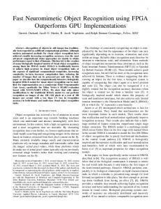
(c) Fig. 1. (a) Part of a CD cover with SURF features. (b) Another view of the CD cover. (c) Matching SURF features between (a) and (b).
Fig. 2. CD cover recognition using a mobile phone.
Fig. 1(a)-(b) shows SURF features overlaid on top of two images, which capture two different views of part of a CD cover. The various features exist at different scales and orientations corresponding to the natural characteristics of this CD cover image. Despite the viewpoint change, many common features are found in both images and can be reliably matched, as depicted in Fig. 1(c). Given a query image, pairwise image matching with every image in the database is an accurate but extremely slow search process, especially if the database size is large. In CD cover recognition on a mobile phone, as depicted in Fig. 2, a mobile phone captures a picture of a CD cover and transmits the query image or features to a server. The server must quickly search through a large database with thousands to millions of CD cover images and return the identity of the query CD cover. Since the user expects a response within a few seconds, the slow pairwise matching would be unacceptable. An effective solution for search through large image databases is to quantize the feature descriptors using a scalable vocabulary tree (SVT) [6]. The SVT is constructed by hierarchical k-means clustering of feature descriptors. The nodes of the tree can be interpreted as a visual dictionary, analogous to a dictionary used for text classification. After quantizing each feature descriptor to the nearest nodes in the SVT, a feature set is efficiently summarized by a tree histogram, expressing how often each tree node is visited. The compactness of the tree histogram is the reason why SVTs enable fast searches through large databases. Treating the tree histogram itself as a high dimensional feature vector, we can consider maximum-margin classification of tree histograms. In [7], local features are quantized to a flat vocabulary, as opposed to the hierarchical vocabulary contained in an SVT. The authors of [7] apply support vector machine (SVM) classification of histograms formed from the flat vocabulary. In our project, we generalize their method to work for SVM classification of tree histograms formed from a hierarchical vocabulary. The tree histogram of [6] discards all geometrical relationships between features. Thus, it is possible for the configuration of keypoints in the top database images after the SVT search to differ from
the configuration of keypoints in the query image. When this occurs, it is better to declare no match than to report a likely false positive match. Thus, we further propose a geometric consistency check after the SVT search. If no strong geometric correspondence is found, we can avoid false positives by reporting no match. We evaluate two different geometric verification algorithms: (1) a very accurate affine consistency check, and (2) a much faster but nearly as accurate scale consistency check. Our report is organized as follows. Sec. 2 reviews how a tree histogam is generated and presents a multi-class extension of the two-class Naive Bayes multivariate model. Then, Sec. 3 presents several different kernels for SVM classification of tree histograms. After SVM classification, the top database images are checked for geometric consistency with the query image using one of two different algorithms, as discussed in Sec. 4. We present experimental results in Sec. 5 for two image databases and evaluate the classification performance of the different kernels and geometric verification algorithms.
(a)
2. BACKGROUND ON TREE HISTOGRAMS 2.1. Tree Histograms in a Scalable Vocabulary Tree A scalable vocabulary tree (SVT) is generated by hierarchical kmeans clustering of training feature descriptors. Hierarchical kmeans is a generalization of the flat k-means algorithm presented in Lecture Notes 7. Fig. 3 illustrates the process of hierarchical k-means clustering of feature descriptors. First, we extract a representative subset of descriptors, usually on the order of several million, from the database images. Second, we perform flat k-means clustering on all these descriptors, resulting in k different clusters. Third, we further perform flat k-means clustering on each of the k clusters, and we repeat this subdivision process recursively until each cluster contains only a few descriptors. A tree structure naturally emerges, where the nodes in the tree are the cluster centroids determined by hierarchical k-means. An example of a small SVT is shown in Fig. 4. In practice, SVTs are grown to be very large, e.g., contain on the order of 1 million leaf nodes, to ensure that the visual vocabulary provides good coverage of the high-dimensional space of feature descriptors. For classification of feature descriptors, we interpret the tree nodes as visual words. Analogous to the multivariate event model shown for text classification in Lecture Notes 2, we define the tree histogram for an image as a vector of node visit counts: x = [x1 x2 · · · xN ], where xi is the number of feature descriptors in the image quantized by nearest-neighbor search to the ith node of the SVT and N is the total number of nodes in the SVT. In the remainder of this report, we will create efficient classifiers for the tree histogram. 2.2. Naive Bayes Classifier As a simple baseline system, we can apply Naive Bayes classification to decide the class of each query image. We generalize the multinomial event model presented in Lecture Notes 2 to the multiclass scenario. During training, we first calculate the prior probability of each class φy=c for c = 1, 2, · · · , C: φy=c
=
m o 1 X n (i) 1 y =c m i=1
.
(1)
We assume there are sufficient training samples in each class so that Laplace smoothing of the prior probabilities is unnecessary. Then,
(b)
(c) Fig. 3. Steps in hierarchical k-means clustering of feature descriptors. (a) Extract feature descriptors from training database images. (b) Perform first level of k-means clustering. (c) Perform second level of k-means clustering.
we calculate the Laplace-smoothed probabilty of the occurence of each tree node or visual word given the class of the image, using the tree histogram x. For c = 1, 2, · · · , C and k = 1, 2, · · · , N , ” “P (i) m (i) +1 1{y = c}x k i=1 ´ φk|y=c = `Pm , (2) (i) = c}ni + N i=1 1 {y
where N is the number of tree nodes or visual words, ni is the number of feature descriptors in the ith image, and C is the number of (i) classes. In the numerator of Eq. 2, xk is the number of times the ith image’s feature descriptors visit the kth node of the SVT. During testing, for a new query image’s tree histogram x, we look for c ∈ {1, · · · , C} that maximizes the following probability: Pr(y = c, x)
=
Pr(y = c)
n Y
Pr(xi |y = c)
i=1
=
φy=c
n Y
i=1
i φxi|y=c
,
(3)
Fig. 4. SVT of depth D = 3 and branch factor k = 3, containing N = 13 nodes. where n is the number of feature descriptors in the query image. Results for Naive Bayes classification of an actual image set will be given in Sec. 5. 3. SUPPORT VECTOR MACHINE CLASSIFICATION OF TREE HISTOGRAMS In this section, we create maximum-margin classifiers for the tree histogram defined in Sec. 2. Our approach is inspired by the prior work in [7], which proposed SVM classifiers for flat visual vocabularies. We generalize their method to work for the hierarchical visual vocabulary contained in an SVT, taking into special account the informativeness of different nodes in the SVT. 3.1. Weighted Tree Histogram In a hierarchical visual vocabulary, it is important to consider the varying degrees of informativeness provided by words at different levels. Intuitively, the nodes at higher levels of the SVT are less informative, because many feature descriptors from many image classes visit them. The analogy in text classification is that a word like mammal is less informative or specific than words like canine and feline. To express this intuition mathematically, we apply a weighting scheme from information retrieval [6] which assigns a informativeness score to each word in a vocabulary: wi = ln (M/Mi )
,
(4)
where M is the total number of training images and Mi is the number of training images that visit the ith word in the visual vocabulary, or the ith word in the SVT. If Mi = 0, which occurs rarely for degenerate parts of the tree, we assign wi = 0 to effectively prune away that part of the tree. This weighting gives greater emphasis to tree nodes visited by fewer images, which are more discriminative in classification. Using the weights defined in Eq. 4, we can create a weighted tree histogram x ˜ = [x1 w1 x2 w2 · · · xN wN ]. The weighted tree histogram is the feature vector we will subsequently use for SVM classification. 3.2. Kernels for SVM Classification We consider four kernels for SVM classifcation of the weighted tree histogram. The simplest is the linear kernel: T
Klin (˜ x, z˜) = x ˜ z˜ .
(5)
The linear kernel is not able to capture correlations between different words in the vocabulary. For example, features associated with the
eyes of a person usually occur together in the same image with features of the nose, ears, mouth, and hair. To exploit such co-occurence relationships while still keeping the complexity of the SVM classifier low, we propose three computationally efficient nonlinear kernels. A polynomial kernel, a Gaussian kernel with L2-norm distance, and a sigmoid kernel are specified as follows: “ ”d Kpoly (˜ x, z˜) = x ˜T z˜ + c , (6) « „ 2 ||˜ x − z˜||2 , (7) KGauss (˜ x, z˜) = exp − σ2 “ ” Ksgm (˜ x, z˜) = tanh x ˜T z˜ + c , (8) where the various parameters in the kernels are selected by ten-fold cross validation. All of these kernels are proven to be Mercer kernels in [8]. Unlike the two-class SVM presented in Lecture Notes 3, we need a more general C-class SVM to classify our image data. We choose the one-versus-one method, where a different SVM is trained between every pair of classes. For C classes, there are C(C − 1)/2 pairs of classes. To classify an image, we perform C(C − 1)/2 comparisons (SVM classifications) and pick the class that wins the majority of comparisons. Experimental results for all the kernels on a real image set is presented in Sec. 5. 4. GEOMETRIC CONSISTENCY CHECK To reduce the number of false positive image matches after SVM classification of the tree histogram, a geometric consistency check between the top database images and the query image should be performed. If no good geometric correspondence is found, no match is reported to reduce the false positive rate. In an application like CD cover recognition, if the classification result is ambiguous, it is better to report no match and prompt the user to try taking another query photo than to report a false CD cover identity. Here, we evaluate two different geometry verification algorithms: an accurate affine consistency check and a much faster but nearly as accurate scale consistency check. 4.1. Affine Consistency Check n
q Let the query image have feature keypoints Pq = {(xq,i , yq,i )}i=1 nd and a database image have keypoints Pd = {(xd,i , yd,i )}i=1 . If the two images contain similar objects and do not differ in viewpoint significantly, a subset of the points in Pq will be well mapped by an affine transformation into a subset of the points in Pd . These affinerelated points are called inliers of the affine model, as opposed to the other points in Pq and Pd called outliers which do not conform to the affine model. The key challenge is to find the best affine transformation when initially we do not know the separation between inliers and outliers. Random sample consensus (RANSAC) [9] is an iterative algorithm well-suited to discovery of unknown models in the presence of outliers. We apply RANSAC to find the best affine transformation between Pq and Pd as follows. Notationally, let |A| denote the size of a set A.
1. For each descriptor vq,i in the query image, find the closest descriptor vd,i∗ in terms of Euclidean distance in the database image. Propose that keypoint (xq,i , yq,i ) ∈ Pq is matched to keypoint (xd,i∗ , yd,i∗ ) ∈ Pd . 2. Initialize RANSAC by setting the following parameters:
(a) max-iteration := maximum number of iterations (b) min-error := ∞. (c) min-start := 3, minimum number of inliers at start (d) min-end := minimum number of inliers for convergence (e) max-offset := a keypoint’s maximum offset from affine model prediction to remain an inlier 3. for (iteration = 1; iteration ≤ max-iteration; iteration++) (a) Set maybe-inliers := min-start random matches. (b) Set maybe-model := least-squares affine model Amaybe between keypoint matches in maybe-inliers (c) Set consensus-set := maybe-inliers (d) For every keypoint (xq,i , yq,i ) ∈ Pq not in maybeinliers, find (ˆ xd,i∗ , yˆd,i∗ ) = Amaybe (xq,i , yq,i ). If the offset ||(xd,i∗ , yd,i∗ ) − (ˆ xd,i , yˆd,i )||2 < max-offset, add this keypoint match to consensus-set.
5. EXPERIMENTAL RESULTS Classification using Naive Bayes and SVMs is performed on two different image databases. The first database is the well-known Zurich Buildings Database (ZuBuD) [10], which contains 1005 database images representing 5 views of 201 buildings in Zurich. The query image set contains 115 images depicting a subset of the 201 buildings. Some examples are shown in Fig. 5. The second database is our own CD Cover Database (CDCD), which contains 3000 database images representing 5 views of 600 CD covers. The query image set consists of 50 images, representing 50 different CD covers drawn randomly from the 600 CD covers. CDCD is more challenging than ZuBuD because of increased background clutter, partial occlusions, and specular reflections from camera flash. Some examples are shown in Fig. 6.
(e) If |consensus-set| < min-end, skip to the next iteration. (f) Set better-model := least-squares affine model Abetter between keypoint matches in consensus-set. (g) For every match in consensus-set, find the offset ||(xd,i∗ , yd,i∗ ) − (ˆ xd,i , yˆd,i )||2 . Set mean-offset := average of these offsets.
Fig. 5. Zurich Building Database images.
(h) If mean-offset < min-error, set min-error := meanoffset, best-model := better-model, and best-consensusset := consensus-set. A correct image match will have a large number of elements in best-consensus-set, whereas an incorrect match will yield very few elements in best-consensus-set. Thus, if |best-consensus-set| is below some minimum threshold, we judge the query and database image to be geometrically dissimilar. The main drawback of the algorithm is its need to repeatedly compute affine models, which makes the algorithm slow and therefore unattractive for low-latency object recognition applications. Thus, in the next section, we propose a more computationally efficient geometric check. 4.2. Scale Consistency Check Assume a query image and a database image share common objects, but the objects may be shown at different magnifications in the two images. Then, the scales {σq,1 , · · · , σq,nq } of features in the query image should be nearly proportional to the scales {σd,1 , · · · , σd,nq } of matching features in the database image. In other words, the ratio of scales {σq,1 /σd,1 , · · · , σq,nq /σd,nq } should be nearly constant. Using this rationale, we propose a scale consistency check. 1. Perform Step 1 of the affine consistency check. 2. Set R := {σq,1 /σd,1 , · · · , σq,nq /σd,nq }. 3. Set rmed := median (R). 4. Set consensus-set := all ratios in R that are within ǫ of rmed . Similar to before, |consensus-set| measures the strength of the geometric correspondence between the query and database images. The reason for choosing the median ratio rather than mean ratio is that the median is less sensitive to outliers. Unlike affine consistency check, scale consistency check is non-iterative and requires much simpler computation. In Sec. 5, we evaluate the two geometric verification algorithms and show scale consistency check performs nearly as well as affine consistency check but runs considerably faster.
Fig. 6. CD Cover Database images. First, we evaluate classification performance without any postSVT geometric verification. We choose SURF over SIFT because SURF has lower dimensionality, enabling our learning algorithms to run faster. Our hierarchical k-means algorithm uses VLFEAT [11] and our SVM algorithm uses LIBSVM [12]. After training Naive Bayes and SVM classifiers on the database images, the performance is tested on the query images. Table 1 compares the match rates for different classifiers, where the match rate (MR) is defined to be MR =
no. query images correctly identified no. query images
(9)
The best performance is obtained for the SVM with a polynomial kernel of degree 10. The polynomial kernel slightly improves classification accuracy compared to the linear kernel for ZuBuD, but the two kernels give the same result for CDCD. Because the tree histograms are already very high-dimensional vectors, there is already sufficient separability between most image classes in the original vector space, allowing the linear kernel to be effective. As expected, the match rates are lower for CDCD than for ZuBuD because CDCD contains more challenging image distortions. Reasonably high match rates are obtained for both databases using SVMs. Naive Bayes performs poorly for CDCD because of the more challenging image distortions, lower ratio of number of foreground features to number of background features, and larger number of classes.
6. CONCLUSION
Table 1. Match rates for ZuBuD and CDCD. ZuBuD Classifier Naive Bayes SVM with Linear Kernel SVM with Gaussian Kernel SVM with Sigmoid Kernel SVM with Degree-10 Polynomial Kernel
MR 0.8957 0.9217 0.9217 0.9217 0.9739
CDCD Classifier Naive Bayes SVM with Linear Kernel SVM with Gaussian Kernel SVM with Sigmoid Kernel SVM with Degree-10 Polynomial Kernel
MR 0.0600 0.8800 0.8800 0.8800 0.8800
This report has presented SVM classification of tree histograms generated from an SVT. We have demonstrated how to generalize SVM classification of flat visual vocabularies to SVM classification of hierarchical vocabularies. Several computationally efficient kernels are suggested. A baseline Naive Bayes classifier was also investigated. Our proposed classifiers are evaluated using two image data sets, the Zurich Building Database and our own more challenging CD Cover Database. The SVM classifiers achieve fairly high match rates for both data sets. On top of the basic SVM classifier, we also proposed geometric verification, with either an affine consistency check or a scale consistency check, to reduce the false positive rate. 7. ACKNOWLEDGMENTS The students would like to thank Prof. Andrew Ng and the teaching assistants for their help and advice. We enjoyed taking the class and are thankful for the opportunity to apply our new machine learning knowledge in this project.
Second, we evaluate the performance of the two proposed geometric verification algorithms and measure the reduction in the false positive rate. If a query image and one of the top post-SVT database images pass the geometric check, we report the result as a match. Otherwise, the result is no match. Then, the false positive rate (FPR) is defined to be FPR =
no. match query images incorrectly identified no. match query images
(10)
Because the polynomial kernel achieved the best result for both databases, we apply geometric consistency check to the polynomial kernel’s top five database images. The comparison of match rates and false positive rates for with and without geometric checks is given in Table 2. We see that for both databases, the false positive rate is reduced significantly by applying a geometric check. The match rate is only reduced slightly for ZuBuD and is unaffected for CDCD, meaning a geometric check rarely discounts valid matches. Also, when measuring the runtime per query image, the scale check runs much faster than the affine check while achieving about the same accuracy.
Table 2. Geometric check results for ZuBuD and CDCD. Geometric Check None Affine Scale
ZuBuD MR FPR 0.9739 0.0087 0.9565 0.0000 0.9739 0.0000
Time (sec) —— 2.5016 1.4887
Geometric Check None Affine Scale
CDCD MR 0.8800 0.8800 0.8800
Time (sec) —— 0.9135 0.3766
FPR 0.0800 0.0417 0.0417
8. REFERENCES [1] G. Fritz, C. Seifert, and L. Paletta, “A mobile vision system for urban detection with informative local descriptors,” in IEEE International Conference on Computer Vision Systems, 2006. [2] H. Bay, B. Fasel, and L. V. Gool, “Interactive museum guide: Fast and robust recognition of museum objects,” in International Workshop on Mobile Vision, 2006. [3] S. Tsai, D. Chen, J. Singh, and B. Girod, “Rate-efficient, realtime CD cover recognition on a camera-phone,” in ACM Multimedia, October 2008. [4] D. Lowe, “Distinctive image features from scale-invariant keypoints,” International Journal of Computer Vision, vol. 60, no. 2, pp. 91–110, November 2004. [5] H. Bay, T. Tuytelaars, and L. V. Gool, “SURF: speeded up robust features,” in European Conference on Computer Vision, May 2006. [6] D. Nister and H. Stewenius, “Scalable recognition with a vocabulary tree,” in IEEE Computer Vision and Pattern Recognition or CVPR, 2006. [7] J. Zhang, M. Marszalek, S. Lazebnik, and C. Schmid, “Local features and kernels for classification of texture and object categories,” in IEEE Computer Vision and Pattern Recognition Workshop, 2006. [8] J. Shawe-Taylor and N. Cristianini, Kernel Methods for Pattern Analysis, Cambridge University Press, 2004. [9] M. A. Fischler and R. C. Bolles, “Random sample consensus: a paradigm for model fitting with applications to image analysis and automated cartography,” Communications of ACM, vol. 24, no. 6, pp. 381–395, June 1981. [10] H. Shao, T. Svoboda, and L. V. Gool, ZuBuD - Zurich Buildings Database for Image Based Recognition, April 2003. [11] A. Vedaldi and B. Fulkerson, VLFEAT - An Open and Portable Library of Computer Vision Algorithms, 2008. [12] C.-C. Chang and C.-J. Lin, LIBSVM - A Library for Support Vector Machines, 2001.