spreads data across banks with a fixed line-bank mapping, and exposes a ... be beneficial because applications vary widely in how well they use the cache.
Appears in the Proceedings of the 21st International Symposium on High Performance Computer Architecture (HPCA), 2015
Scaling Distributed Cache Hierarchies through Computation and Data Co-Scheduling Nathan Beckmann, Po-An Tsai, Daniel Sanchez Massachusetts Institute of Technology {beckmann, poantsai, sanchez}@csail.mit.edu
optimization problem. We have developed CDCS, a scheme that performs computation and data co-scheduling effectively on modern CMPs. CDCS uses novel, efficient heuristics that achieve performance within 1% of impractical, idealized solutions. CDCS works on arbitrary mixes of single- and multi-threaded processes, and uses a combination of hardware and software techniques. Specifically, our contributions are: • We develop a novel thread and data placement scheme that takes into account both data allocation and access intensity to jointly place threads and data across CMP tiles (Sec. IV). • We design miss curve monitors that use geometric sampling to scale to very large NUCA caches efficiently (Sec. IV-G). • We present novel hardware that enables incremental reconfigurations of NUCA caches, avoiding the bulk invalidations and long pauses that make reconfigurations expensive in prior NUCA techniques [4, 20, 41] (Sec. IV-H). We prototype CDCS on Jigsaw [4], a partitioned NUCA baseline (Sec. III), and evaluate it on a 64-core system with lean OOO cores (Sec. VI). CDCS outperforms an S-NUCA cache by 46% gmean (up to 76%) and saves 36% of system energy. CDCS also outperforms R-NUCA [20] and Jigsaw [4] under different thread placement schemes. CDCS achieves even higher gains in under-committed systems, where not all cores are used (e.g., due to serial regions [25] or power caps [17]). CDCS needs simple hardware, works transparently to applications, and reconfigures the full chip every few milliseconds with minimal software overheads (0.2% of system cycles).
Abstract—Cache hierarchies are increasingly non-uniform, so for systems to scale efficiently, data must be close to the threads that use it. Moreover, cache capacity is limited and contended among threads, introducing complex capacity/latency tradeoffs. Prior NUCA schemes have focused on managing data to reduce access latency, but have ignored thread placement; and applying prior NUMA thread placement schemes to NUCA is inefficient, as capacity, not bandwidth, is the main constraint. We present CDCS, a technique to jointly place threads and data in multicores with distributed shared caches. We develop novel monitoring hardware that enables fine-grained space allocation on large caches, and data movement support to allow frequent full-chip reconfigurations. On a 64-core system, CDCS outperforms an S-NUCA LLC by 46% on average (up to 76%) in weighted speedup and saves 36% of system energy. CDCS also outperforms state-of-the-art NUCA schemes under different thread scheduling policies. Index Terms—cache, NUCA, thread scheduling, partitioning
I. I NTRODUCTION
The cache hierarchy is one of the main performance and efficiency bottlenecks in current chip multiprocessors (CMPs) [13, 21], and the trend towards many simpler and specialized cores further constrains the energy and latency of cache accesses [13]. Cache architectures are becoming increasingly non-uniform to address this problem (NUCA [34]), providing fast access to physically close banks, and slower access to far-away banks. For systems to scale efficiently, data must be close to the computation that uses it. This requires keeping cached data in banks close to threads (to minimize on-chip traffic), II. BACKGROUND AND I NSIGHTS while judiciously allocating cache capacity among threads (to minimize cache misses). Prior work has attacked this problem We now discuss the prior work related to computation and in two ways. On the one hand, dynamic and partitioned NUCA data co-scheduling, focusing on the techniques that CDCS draws techniques [2, 3, 4, 8, 10, 11, 20, 28, 42, 51, 63] allocate cache from. First, we discuss related work in multicore last-level space among threads, and then place data close to the threads caches (LLCs) to limit on- and off-chip traffic. Next, we present that use it. However, these techniques ignore thread placement, a case study that compares different NUCA schemes and shows which can have a large impact on access latency (Sec. II-B). that thread placement significantly affects performance. Finally, On the other hand, thread placement techniques mainly focus we review prior work on thread placement and show that NUCA on non-uniform memory architectures (NUMA) [7, 14, 29, presents an opportunity to improve thread placement beyond 57, 59, 64] and use policies, such as clustering, that do not prior schemes. translate well to NUCA. In contrast to NUMA, where capacity is plentiful but bandwidth is scarce, capacity contention is the A. Multicore caches main constraint for thread placement in NUCA (Sec. II-B). Non-uniform cache architectures: NUCA techniques [34] are We find that to achieve good performance, the system concerned with data placement, but do not place threads or must both manage cache capacity well and schedule threads divide cache capacity among them. Static NUCA (S-NUCA) [34] to limit capacity contention. We call this computation and spreads data across banks with a fixed line-bank mapping, and data co-scheduling. This is a complex, multi-dimensional exposes a variable bank latency. Commercial CMPs often use 1
Legend Tile (1 core+LLC bank) Thread running on core LLC data breakdown
(a) R-NUCA
Example I1 (ilbdc) thread Data from O1 and O2
omnet
Threads Data
ilbdc
(b) Jigsaw+Clustered
Threads Data
x8
x8
(c) Jigsaw+Random
Threads
milc Data
………
(d) CDCS
Figure 1: Case study: 36-tile CMP with a mix of single- and multi-threaded workloads (omnet×6, milc×14, 8-thread ilbdc×2) under different NUCA organizations and thread placement schemes. Threads are labeled and data is colored by process.
dp WS p
mi
lc
omnet milc ilbdc
ilb
MPKI
place data close to the requesting core [2, 3, 8, 10, 11, 20, 28, 42, 51, 63] using a mix of placement, migration, and replication techniques. Placement and migration bring lines close to cores that use them, possibly introducing capacity contention between cores depending on thread placement. Replication makes multiple copies of frequently used lines, reducing latency for widely read-shared lines (e.g., hot code) at the expense of some capacity loss. Most D-NUCA designs build on a private-cache baseline, where each NUCA bank is treated as a private cache. All banks are under a coherence protocol, which makes such schemes either hard to scale (in snoopy protocols) or require large directories that incur significant area, energy, latency, and complexity overheads (in directory-based protocols). To avoid these costs, some D-NUCA schemes instead build on a shared-cache baseline: banks are not under a coherence protocol, and virtual memory is used to place data. Cho and Jin [11] use page coloring to map pages to banks. R-NUCA [20] specializes placement and replication policies for different data classes (instructions, private data, and shared data), outperforming prior D-NUCA schemes. Shared-baseline schemes are cheaper, as LLC data does not need coherence. However, remapping data is expensive as it requires page copies and invalidations. Partitioned shared caches: Partitioning enables software to explicitly allocate cache space among threads or cores, but it is not concerned with data or thread placement. Partitioning can be beneficial because applications vary widely in how well they use the cache. Cache arrays can support multiple partitions with small modifications [9, 38, 40, 53, 56, 62]. Software can then set these sizes to maximize throughput [52], or to achieve fairness [44], isolation and prioritization [12, 18, 32], and security [47]. Unfortunately, partitioned caches scale poorly because they do not optimize placement. Moreover, they allocate capacity to cores, which works for single-threaded mixes, but incorrectly accounts for shared data in multi-threaded workloads. Partitioned NUCA: Recent work has developed techniques to perform spatial partitioning of NUCA caches. These schemes
80
om net
100
dc
120
S-NUCA [35]. Dynamic NUCA (D-NUCA) schemes adaptively
R-NUCA
1.09
0.99
1.15
1.08
Jigsaw+Cl Jigsaw+Rnd
2.88 3.99
1.40 1.20
1.21 1.21
1.48 1.47
CDCS
4.00
1.40
1.20
1.56
60 40 20 0 0.0 0.5 1.0 1.5 2.0 2.5 3.0 3.5 4.0
LLC Size (MB)
Figure 2: Application Table 1: Per-app and weighted speedups for the mix studied. miss curves. jointly consider data allocation and placement, reaping the benefits of NUCA and partitioned caches. However, they do not consider thread placement. Virtual Hierarchies rely on a logical two-level directory to partition the cache [41], but they only allocate full banks, double directory overheads, and make misses slower. CloudCache [36] implements virtual private caches that can span multiple banks, but allocates capacity to cores, needs a directory, and uses broadcasts, making it hard to scale. Jigsaw [4] is a shared-baseline NUCA with partitionable banks and single-lookup accesses. Jigsaw lets software divide the distributed cache in finely-sized virtual caches, place them in different banks, and map pages to different virtual caches. Using utility monitors [52], an OS-level software runtime periodically gathers the miss curve of each virtual cache and co-optimizes data allocation and placement. B. Case study: Tradeoffs in thread and data placement To explore the effect of thread placement on different NUCA schemes, we simulate a 36-core CMP running a specific mix. The CMP is a scaled-down version of the 64-core chip in Fig. 3, with 6×6 tiles. Each tile has a simple 2-way OOO core and a 512 KB LLC bank. (See Sec. V for methodology details.) We run a mix of single- and multi-threaded workloads. From single-threaded SPEC CPU2006, we run six instances of omnet (labeled O1-O6) and 14 instances of milc (M1-M14). From multi-threaded SPEC OMP2012, we run two instances of ilbdc (labeled I1 and I2) with eight threads each. We choose this mix because it illustrates the effects of thread and data placement— Sec. VI uses a comprehensive set of benchmarks. Fig. 1 shows how thread and data are placed across the chip under different schemes. Each square represents a tile. The 2
label on each tile denotes the thread scheduled in the tile’s now have their data in neighboring banks (1.2 hops on average, core (labeled by benchmark as discussed before). The colors instead of 3.2 hops in Fig. 1b) and enjoy a 3.99× speedup over on each tile show a breakdown of the data in the tile’s bank. S-NUCA. Unfortunately, ilbdc’s threads are spread further, and Each process uses the same color for its threads and data. its performance suffers relative to clustering threads (Table 1). For example, in Fig. 1b, the upper-leftmost tile has thread O1 This shows why one policy does not fit all: depending on (colored blue) and its data (also colored blue); data from O1 capacity contention and sharing behavior, apps prefer different also occupies parts of the top row of banks (portions in blue). placements. Specializing policies for single- and multithreaded Fig. 1a shows the thread and data breakdown under R-NUCA apps would only be a partial solution, since multithreaded apps when applications are grouped by type (e.g., the six copies of with large per-thread footprints and little sharing also benefit omnet are in the top-left corner). R-NUCA maps thread-private from spreading. data to each thread’s local bank, resulting in very low latency. Finally, Fig. 1d shows how CDCS handles this mix. CDCS Banks also have some of the shared data from the multithreaded spreads omnet instances across the chip, avoiding capacity processes I1 and I2 (shown hatched), because R-NUCA spreads contention, but clusters ilbdc instances across their shared shared data across the chip. Finally, code pages are mapped to data. CDCS achieves a 4× speedup for omnet and a 40% different banks using rotational interleaving, though this is not speedup for ilbdc. CDCS speeds up this mix by 56%. visible in this mix because apps have small code footprints. In summary, this case study shows that partitioned NUCA These policies excel at reducing LLC access latency to private schemes use capacity more effectively and improve perfordata vs. an S-NUCA cache. This helps milc and omnet, as mance, but they are sensitive to thread placement, as threads shown in Table 1. Overall, R-NUCA speeds up this mix by 8% in neighboring tiles can aggressively contend for capacity. This over S-NUCA. presents an opportunity to perform smart thread placement, but In R-NUCA, other thread placements would make little fixed policies have clear shortcomings. difference for this mix, as most capacity is used for either thread-private data, which is confined to the local bank, or C. Cache and NUMA-aware thread placement shared data, which is spread out across the chip. But R-NUCA CRUISE [29] is perhaps the closest work to CDCS. CRUISE does not use capacity efficiently in this mix. Fig. 2 shows why, schedules single-threaded apps in CMPs with multiple fixedgiving the miss curves of each app. Each miss curve shows size last-level caches, each shared by multiple cores and the misses per kilo-instruction (MPKI) that each process incurs unpartitioned. CRUISE takes a classification-based approach, as a function of LLC space (in MB). omnet is very memorydividing apps in thrashing, fitting, friendly, and insensitive, intensive, and suffers 85 MPKI below 2.5 MB. However, over and applies fixed scheduling policies to each class (spreading 2.5 MB, its data fits in the cache and misses turn into hits. some classes among LLCs , using others as filler, etc.). CRUISE ilbdc is less intensive and has a smaller footprint of 512 KB. bin-packs apps into fixed-size caches, but partitioned NUCA Finally, milc gets no cache hits no matter how much capacity schemes provide flexibly sized virtual caches that can span it is given—it is a streaming application. In R-NUCA, omnet multiple banks. It is unclear how CRUISE ’s policies and and milc apps get less than 512 KB, which does not benefit classification would apply to NUCA . For example, CRUISE them, and ilbdc apps use more capacity than they need. would classify omnet as thrashing if it was considering many Jigsaw uses capacity more efficiently, giving 2.5 MB to each small LLCs , and as insensitive if considering few larger LLCs. instance of omnet, 512 KB to each ilbdc (8 threads), and nearCRUISE improves on DI [64], which profiles miss rates and zero capacity to each milc. Fig. 1b shows how Jigsaw tries to schedules apps across chips to balance intensive and nonplace data close to the threads that use it. By using partitioning, Jigsaw can share banks among multiple types of data without intensive apps. Both schemes only consider single-threaded introducing capacity interference. However, the omnet threads apps, and have to contend with the lack of partitioned LLCs. in the corner heavily contend for capacity of neighboring Other thread placement schemes focus on NUMA systems. banks, and their data is placed farther away than if they NUMA techniques have different goals and constraints than were spread out. Clearly, when capacity is managed efficiently, NUCA: the large size and low bandwidth of main memory limit thread placement has a large impact on capacity contention reconfiguration frequency and emphasize bandwidth contention and achievable latency. Nevertheless, because omnet’s data over capacity contention. Tam et al. [57] profile which threads now fits in the cache, its performance vastly improves, by have frequent sharing and place them in the same socket. 2.88× over S-NUCA (its AMAT improves from 15.2 to 3.7 DINO [7] clusters single-threaded processes to equalize memory cycles, and its IPC improves from 0.22 to 0.61). ilbdc is also intensity, places clusters in different sockets, and migrates pages faster, because its shared data is placed close by instead of along with threads. In on-chip NUMA (CMPs with multiple across the chip; and because omnet does not consume memory memory controllers), Tumanov et al. [59] and Das et al. [14] bandwidth anymore, milc instances have more of it and speed profile memory accesses and schedule intensive threads close up moderately (Table 1). Overall, Jigsaw speeds up this mix to their memory controller. These NUMA schemes focus on by 48% over S-NUCA. equalizing memory bandwidth, whereas we find that proper Fig. 1c shows the effect of randomizing thread placement to cache allocations cause capacity contention to be the main spread capacity contention among the chip. omnet instances constraint on thread placement. 3
Tile Organization
64-tile CMP Memory controller
Virtual-cache-to-bank Translation Buffer (VTB)
Bank Partitioning
Tile
Memory controller
Memory controller
Monitoring
Move Control
0x5CA1AB1E VC descriptor Bank/ Part 0
Router
L2 L1I
VTB
L1D Core
Memory controller
2706
CDCS hardware support
Example LLC Access Tile 3
Address (from L1 miss)
VC id (from TLB)
LLC Bank
1/3
VTB Entry
3 entries, associative, Shadow exception on miss descriptor (for moves)
H 1
3/5
1/3
… …
Bank/ Part N-1
0/8
0x5CA1AB1E maps to bank 3, bank part 5
CDCS LLC Bank 3 4 LLC Hit Update part 5 counters Add core 0 sharer 3 L2 Miss CDCS LLC lookup, bank 3, bank partition 5 2 L1D Miss L2 and VTB lookup 1 LD 0x5CA1AB1E
5 Serve line
NoC 3 5
GETS
VTB
0x5CA1AB1E
L2
L1D TLBs
L1D
Core 0 Tile 0
Figure 3: Target CMP (left), with tile configuration and microarchitectural additions introduced for CDCS. CDCS gangs portions of banks into virtual caches, and uses the VTB (center) to find the bank and bank partition to use on each access (right).
Finally, prior work has used high-quality static mapping techniques to spatially decompose regular parallel problems. Integer linear programming is useful in spatial architectures [45], and graph partitioning is commonly used in stream scheduling [49, 50]. While some of these techniques could be applied to the thread and data placement problem, they are too expensive to use dynamically, as we will see in Sec. VI-C.
The virtual-cache translation buffer (VTB), shown in Fig. 3, determines the bank and bank partition for each access. The VTB stores the configuration of all VCs that the running thread can access [4]. In our implementation, it is a 3-entry lookup table, as each thread only accesses 3 VCs (as explained below). Each VTB entry contains a VC descriptor, which consists of an array of N bank and bank partition ids (in our implementation, N = 64 buckets). As shown in Fig. 3, to find the bank and III. CDCS O PERATION bank partition ids, the address is hashed, and the hash value Because Sec. II-B shows that judicious, fine-grained capacity (between 0 and N − 1) selects the bucket. Hashing allows allocation is highly beneficial, we adopt some of Jigsaw’s spreading accesses across the VC’s bank partitions in proportion mechanisms as a baseline for CDCS. We first explain how to their capacities, which makes them behave as a cache of CDCS operates between reconfigurations (similar to Jigsaw), their aggregate size. For example, if a VC consists of two bank then how reconfigurations happen in Sec. IV (different from partitions A of 1 MB and B of 3 MB, by setting array elements Jigsaw). For ease of understanding, we present CDCS in the 0–15 in the VC descriptor to A and elements 16–63 to B, concrete context of a partitioned NUCA scheme. In Sec. IV-I, B receives 3× more accesses than A. In this case, A and B we discuss how to generalize CDCS to other NUCA substrates. behave like a 4 MB VC [4, 5]. Fig. 3 shows the tiled CMP architecture we consider, and The VTB is small and efficient. For example, with N = 64 the hardware additions of CDCS. Each tile has a core and a buckets, 64 LLC banks, and 64 partitions per bank, each slice of the LLC. An on-chip network of arbitrary topology VC descriptor takes 96 bytes (64 2×6-bit buckets, for bank connects tiles, and memory controllers are at the edges. Pages and bank partition ids). Each of the 3 VTB entries has are interleaved across memory controllers, as in Tilera and two descriptors (shadow descriptors, shown in Fig. 3, aid Knights Corner chips [6]. In other words, we do not consider on- reconfigurations and are described in Sec. IV-H), making the chip NUMA-aware placement. We focus on NUCA over NUMA VTB ∼600 bytes. Since VTB lookups are cheap, they are because many apps have working sets that fit on-chip, so performed in parallel with L2 accesses, so that L2 misses can be LLC access latency dominates their performance. NUMA-aware routed to the appropriate LLC bank immediately. Fig. 3 (right) placement is complementary and CDCS could be extended to shows how the VTB is used in LLC accesses. also perform it (Sec. II-C), which we leave to future work. Periodically (e.g., every 25 ms), CDCS software changes the Virtual caches: CDCS lets software divide each cache bank in configuration of some or all VCs, changing both their bank multiple partitions, using Vantage [53] to efficiently partition partitions and sizes. The OS recomputes all VC descriptors banks at cache-line granularity. Collections of bank partitions based on the new data placement, and cores coordinate via are ganged and exposed to software as a single virtual cache inter-processor interrupts to update the VTB entries simulta(VC) (called a share in Jigsaw [4]). This allows software to neously. Sec. IV-H details how CDCS hardware incrementally define many VCs cheaply (several per thread), and to finely reconfigures the cache, moving or invalidating lines that size and place them among banks. have changed location to maintain coherence. The two-level Mapping data to VCs: Unlike other D-NUCAs, in CDCS lines translation of pages to VCs and VCs to bank partitions allows do not migrate in response to accesses. Instead, between Jigsaw and CDCS to be more responsive and take more reconfigurations, each line can only reside in a single LLC bank. drastic reconfigurations than prior shared-baseline D-NUCAs: CDCS maps data to VCs using the virtual memory subsystem, reconfigurations simply require changing the VC descriptors, similar to R-NUCA [20]. Each page table entry is tagged with and software need not copy pages or alter page table entries. a VC id. On an L2 miss, CDCS uses the line address and its Types of VCs: CDCS’s OS-level runtime creates one threadVC id to determine the bank and bank partition that the line private VC per thread, one per-process VC for each process, maps to. and a global VC. Data accessed by a single thread is mapped 4
Miss curves
Misses
GMONs
Latencyaware allocation
Virtual Cache (VC) sizes
Optimistic data placement
Thread placement
Refined data placement
Placed VCs and threads
Reconfigure (moves)
Allocated Size
Figure 4: Overview of CDCS’s periodic reconfiguration procedure.
On-chip latency: Each VC’s capacity allocation sP d consists N of portions of the N banks on chip, so that sd = b=1 sd,b . The capacity of each bank B constrains allocations, so that PD B = d=1 sd,b . Limited bank capacities sometimes force data to be further away from the threads that access it, as we saw in Sec. II-B. Because the VTB spreads accesses across banks in proportion to capacity, PD thes number of accesses from thread t to bank b is αt,b = d=1 sd,b × at,d . If thread t is placed in d a core ct and the network distance between two tiles t1 and t2 is D(t1 , t2 ), then the on-chip latency is:
to its thread-private VC, data accessed by multiple threads in the same process is mapped to the per-process VC, and data used by multiple processes is mapped to the global VC. Pages can be reclassified to a different VC efficiently [4] (e.g., when a page in a per-thread VC is accessed by another thread, it is remapped to the per-process VC), though in steady-state this happens rarely. IV. CDCS R ECONFIGURATIONS CDCS reconfigurations use a combination of hardware and software techniques. Fig. 4 gives an overview of the steps involved. Novel, scalable geometric monitors (Sec. IV-G) sample the miss curves of each virtual cache. An OS runtime periodically reads these miss curves and uses them to jointly place VCs and threads using a 4-step procedure. Finally, this runtime uses hardware support to move cache lines to their new locations (Sec. IV-H). We first describe the software algorithm, then the monitoring and reconfiguration hardware. This hardware addresses overheads that would hinder CDCS performance, especially on large systems. However, these hardware techniques are useful beyond CDCS, e.g. to simplify coherence or reduce partitioning overheads. All aspects of this process differ from Jigsaw [4]. Jigsaw uses a simple runtime that sizes VCs obliviously to their latency, places them greedily, and does not place threads. Jigsaw also uses conventional utility monitors [52] that do not scale to large caches, and reconfigurations require long pauses while banks invalidate data, which adds jitter.
On-chip latency =
T X N X
αt,b × D(ct , b)
(2)
t=1 b=1
B. Overview of CDCS reconfiguration steps With this cost model, the computation and data co-scheduling problem is to choose the ct (thread placement) and st,b (VC size and data placement) that minimize total latency, subject to the given constraints. However, finding the optimal solution is NP-hard [24, 48], and different factors are intertwined. For example, the size of VCs and the thread placement affect how close data can be placed to the threads that use it. CDCS takes a multi-step approach to disentangle these interdependencies. CDCS first adopts optimistic assumptions about the contention introduced by thread and data placement, and gradually refines them to produce the final placement. Specifically, reconfigurations consist of four steps: 1) Latency-aware allocation divides capacity among VCs assuming data is compactly placed (no capacity contention). 2) Optimistic contention-aware VC placement places VCs among banks to avoid capacity contention. This step produces a rough picture of where data should be in the chip, e.g. placing omnet VCs far away enough in Fig. 1 to avoid the pathological contention in Fig. 1b. 3) Thread placement uses the optimistic VC placement to place threads close to the VCs they access. For example, in Fig. 1d, this step places omnet applications close to the center of mass of their data, and clusters ilbdc threads around their shared data. 4) Refined VC placement improves on the previous data placement to, now that thread locations are known, place data closer to minimize on-chip latency. For example, a thread that accesses its data intensely may swap allocations with a less intensive thread to bring its data closer; while this increases latency for the other thread, overall it is beneficial. By considering data placement twice (steps 2 and 4), CDCS accounts for the circular relationship between thread and data placement. We were unable to obtain comparable results with a single VC placement; and CDCS performs almost as well as impractically expensive schemes, such as integer linear
A. A simple cost model for thread and data placement As discussed in Sec. II-C, classification-based heuristics are hard to apply to NUCA. Instead, CDCS uses a simple analytical cost model that captures the effects of different placements on total memory access latency, and uses it to find a low-cost solution. This latency is better analyzed as the sum of on-chip (L2 to LLC) and off-chip (LLC to memory) latencies. Off-chip latency: Assume a system with T threads and D VCs. Each thread t accesses VC d at a rate at,d (e.g., 50 K accesses in 10 ms). If VC d is allocated sd lines in the cache, its miss ratio is Md (sd ) (e.g., 10% of accesses miss). Then the total off-chip access latency is: T X D X Off-chip latency = at,d ×Md (sd )×MemLatency (1) t=1 d=1
where MemLatency is the latency of a memory access. This includes network latency, and relies on the average distance of all cores to memory controllers being the same (Fig. 3). Extending CDCS to NUMA would require modeling a variable main memory latency in Eq. 1. 5
Latency (cycles)
Off-chip
0
0
.4
0
0
0
.8
0
0
0
.8
0
0
0
.8
0
0
0
.4
1
.4
0
.8
1
.8
0
.8
1
.8
0
.8
1
.8
0
.4
1
1
1
.4
0
.4
1
.4
0
0
.8
0
1
0
.8
0
1
.6
.8
0
1
0
0
.4
0
0
0
0
1
1
0
0
1
1
1
.6
1
1
On-chip Total
Capacity (bytes)
Figure 5: Access latency vs. capacity allocation.
Figure 6: Optimistic uncontended virtual cache placement.
(a) Partial optimistic data placement
(b) Estimating contention for VC
(c) VC placed near least contended tile
Figure 7: Optimistic, contention-aware virtual cache placement.
programming (Sec. VI-C). CDCS uses arbitrary distance vectors, so it works with arbitrary topologies. However, to make the discussion concrete, we use a mesh topology in the examples.
large VCs close to each other. The main goal of this step is to inform thread placement by avoiding VC placements that produce high capacity contention, as in Fig. 1b. To this end, we sort VCs by size and place the largest ones first. Intuitively, this works well because larger VCs can cause more contention, while small VCs can fit in a fraction of a bank and cause little contention. For each VC, the algorithm iterates over all the banks, and chooses the bank that yields the least contention with already-placed VCs as the center of mass of the current VC. To make this search efficient, we approximate contention by keeping a running tally of claimed capacity in each bank, and relax capacity constraints, allowing VCs to claim more capacity than is available at each bank. With N banks and D VCs, the algorithm runs in O(N · D). Fig. 7 shows an example of optimistic contention-aware VC placement at work. Fig. 7a shows claimed capacity after two VCs have been placed. Fig. 7b shows the contention for the next VC at the center of the mesh (hatched), where the uncontended placement is a cross. Contention is approximated as the claimed capacity in the banks covered by the hatched area—or 3.6 in this case. To place a single VC, we compute the contention around that tile. We then place the VC around the tile that had the lowest contention, updating the claimed capacity accordingly. For instance, Fig. 7c shows the final placement for the third VC in our example.
C. Latency-aware capacity allocation As we saw in Sec. II-B, VC sizes have a large impact on both off-chip latency and on-chip latency. Prior work has partitioned cache capacity to reduce cache misses [4, 52], i.e. off-chip latency. However, it is well-known that larger caches take longer to access [22, 23, 58]. Most prior partitioning work has targeted fixed-size LLCs with constant latency. But capacity allocation in NUCA caches provides an opportunity to also reduce on-chip latency: if an application sees little reduction in misses from a larger VC, the additional network latency to access it can negate the benefits of having fewer misses. In summary, larger allocations have two competing effects: decreasing off-chip latency and increasing on-chip latency. This is illustrated in Fig. 5, which shows the average memory access latency to one VC (e.g., a thread’s private data). Fig. 5 breaks latency into its off- and on-chip components, and shows that there is a “sweet spot” that minimizes total latency. This has two important consequences. First, unlike in other D-NUCA schemes, it is sometimes better to leave cache capacity unused. Second, incorporating on-chip latency changes the curve’s shape and also its marginal utility [52], leading to different cache allocations even when all capacity is used. CDCS allocates capacity from total memory latency curves E. Thread placement (the sum of Eq. 1 and Eq. 2) instead of miss curves. However, Given the previous data placement, CDCS tries to place Eq. 2 requires knowing the thread and data placements, which threads closest to the center of mass of their accesses. Recall are unknown at the first step of reconfiguration. CDCS instead that each thread accesses multiple VCs, so this center of mass uses an optimistic on-chip latency curve, found by compactly is computed by weighting the centers of mass of each VC by placing the VC around the center of the chip and computing the thread’s accesses to that VC. Placing the thread at this the resulting average latency. For example, Fig. 6 shows the center of mass minimizes its on-chip latency (Eq. 2). optimistic placement of an 8.2-bank VC accessed by a single Unfortunately, threads sometimes have the same centers thread, with an average distance of 1.27 hops. of mass. To break ties, CDCS places threads in descending With this simplification, CDCS uses the Peekahead optiintensity-capacity product (sum of VC accesses × VC size for mization algorithm [4] to efficiently find the sizes of all VCs each VC accessed). Intuitively, this order prioritizes threads for that minimize latency. While these allocations account for onwhich low on-chip latency is important, and for which VCs are chip latency, they generally underestimate it due to capacity hard to move. For example, in the Sec. II-B case study, omnet contention. Nevertheless, we find that this scheme works well accesses a large VC very intensively, so omnet instances are because the next steps are effective at limiting contention. placed first. ilbdc accesses moderately-sized shared data at D. Optimistic contention-aware VC placement moderate intensity, so its threads are placed second, clustered Once VC sizes are known, CDCS first finds a rough picture around their shared VCs. Finally, milc instances access their of how data should be placed around the chip to avoid placing private VCs intensely, but these VCs are tiny, so they are placed 6
1 2 3 4
move its data placed in b (if any) closer by iterating over closer, desirable banks and offering trades with VCs that have data in these banks. If the trades are beneficial, they are performed. The spiral terminates when the VC has seen all of its data, since no farther banks will allow it to move any data closer. Fig. 8 illustrates this for an example CMP with four VCs and some initial data placement. We now discuss how CDCS performs a bounded search for VC1. We spiral outward starting from VC1’s center of mass at bank A, and terminate at VC1’s farthest data at bank C. Desirable banks are marked with black checks on the left of Fig. 8. We only attempt a few trades, shown on the right side of Fig. 8. At bank B, VC1’s data is two hops away, so we try to trade it to any closer, marked bank. For illustration, suppose none of the trades are beneficial, so the data does not move. This repeats at bank C, but suppose the first trade is now beneficial. VC1 and VC4 trade capacity, moving VC1’s data one hop closer. This approach gives every VC a chance to improve its placement. Since any beneficial trade must benefit one party, it would discover all beneficial trades. However, for efficiency, in CDCS each VC trades only once, since we have empirically found this discovers most trades. Finally, this scheme incurs negligible overheads, as we will see in Sec. VI-C.
B
C
Trades A
Figure 8: Trading data placement: Starting from a simple initial placement, VCs trade capacity to move their data closer. Only trades that reduce total latency are permitted. last. This is fine because the next step, refined VC placement, can move small VCs to be close to their accessors very easily, with little effect on capacity contention. For multithreaded workloads, this approach clusters sharedheavy threads around their shared VC, and spreads privateheavy threads to be close to their private VCs. Should threads access private and shared data with similar intensities, CDCS places threads relatively close to their shared VC but does not tightly cluster them, avoiding capacity contention among their private VCs. F. Refined VC placement Finally, CDCS performs a round of detailed VC placement to reduce the distance between threads and their data. CDCS first simply round-robins VCs, placing capacity as close to threads as possible without violating capacity constraints. This greedy scheme, which was used in Jigsaw [4], is a reasonable starting point, but produces sub-optimal placements. For example, a thread’s private VC always gets space in its local bank, regardless of the thread’s memory intensity. Also, shared VCs can often be moved at little or no cost to make room for data that is more sensitive to placement. This is because moving shared data farther away from one accessing thread often moves it closer to another. Furthermore, unlike in previous steps, it is straightforward to compute the effects of moving data, since we have an initial placement to compare against. CDCS therefore looks for beneficial trades between pairs of VCs after the initial, greedy placement. Specifically, CDCS computes the latency change from trading capacity between VC1 at bank b1 and VC2 at bank b2 using Eq. 2. The change in latency for VC1 is: � Accesses ∆Latency = × D(VC1 , b1 ) − D(VC1 , b2 ) Capacity The first factor is VC1 ’s accesses per byte of allocated capacity. Multiplying by this factor accounts for the number of accesses that are affected by moving capacity, which varies between VCs. The equation for VC2 is similar, and the net effect of the trade is their sum. If the net effect is negative (lower latency is better), then the VCs swap bank capacity. Na¨ıvely enumerating all possible trades is prohibitively expensive, however. Instead, CDCS performs a bounded search by iterating over all VCs: Each VC spirals outward from its center of mass, trying to move its data closer. At each bank b along the outward spiral, if the VC has not claimed all of b’s capacity then it adds b to a list of desirable banks. These are the banks it will try to trade into later. Next, the VC tries to
These techniques are cheap and effective. We also experimented with more expensive approaches commonly used in placement problems: integer linear programming, simulated annealing, and graph partitioning. Sec. VI-C shows that they yield minor gains and are too expensive to be used online. We now discuss the hardware extensions necessary to efficiently implement CDCS on large CMPs. G. Monitoring large caches Monitoring miss curves in large CMPs is challenging. To allocate capacity efficiently, we should manage it in small chunks (e.g., the size of the L1s) so that it isn’t over-allocated where it produces little benefit. This is crucial for VCs with small working sets, which see large gains from a small size and no benefit beyond. Yet, we also need miss curves that cover the full LLC because a few VCs may benefit from taking most capacity. These two requirements—fine granularity and large coverage—are problematic for existing monitors. Conventional cache partitioning techniques use utility monitors (UMONs) [52] to monitor a fraction of sets, counting hits at each way to gather miss curves. UMONs monitor a fixed cache capacity per way, and would require a prohibitively large associativity to achieve both fine detail and large coverage. Specifically, in an UMON with W ways, each way models 1/W of LLC capacity. With a 32 MB LLC (Sec. V, Table 2) if we want to allocate capacity in 64 KB chunks, a conventional UMON needs 512 ways to have enough resolution. This is expensive to implement, even for infrequently used monitors. Instead, we develop a novel monitor, called a geometric monitor (GMON). GMONs need fewer ways—64 in our evaluation— to model capacities from 64 KB up to 32 MB. This is possible because GMONs vary the sampling rate across ways, giving both fine detail for small allocations and large coverage, while 7
…
Way 0 Address H3
0xFE3D98
0xDD380B
0xB3D3GA
0x0E5A7B
0x123456
0xCDEF00
0x3173FC
0xCDC911
… 0xBAD031
0xADD235
… 0x541302
0x7A5744
True