2000. 2500. 0.001 0.01. 0.1. 1. 10. 100 1000. G avg. , G dev. N. Gavg, [-N:N]. Gdev, [-N:N]. Gavg, [0:N]. Gdev, [0:N]. Figure : Gradients: Iris, Diabetes, Glass, Heart ...
Search Space Boundaries in Neural Network Error Landscape Analysis Anna Bosman, Andries Engelbrecht, Mardé Helbig Computational Intelligence Research Group (CIRG) Department of Computer Science University of Pretoria http://cirg.cs.up.ac.za
SSCI, 2016
Outline 1 FFNNs 2 Error Landscapes 3 Gradients 4 Ruggedness 5 Searchability 6 Conclusions
Feed Forward Neural Networks Training • Minimize the error: PP PK Emse =
p=1
k =1 (tkp
− okp )2
PK
• What kind of function are we dealing with? • How do we adapt a training algorithm to this optimisation problem?
Error Landscapes
Fitness Landscape Analysis • Estimate landscape properties such as ruggedness, neutrality, searchability, etc. • How? By analysing random samples of the search space • Samples must be representative of the problem at hand
NN Error Landscape • Every weight vector is associated with an error value ~ ∈R • Error values of every w make up the error landscape
Research Questions Fitness Landscapes of Neural Networks • Neural Network search space is unbounded • What subspaces are representative/relevant? • How do the landscape properties change based on the bounds chosen?
Experimental Set-Up Benchmarks considered Problem Iris Diabetes Glass Heart
In 4 8 9 32
Hidden 2 6 9 6
Out 3 2 6 1
Dimensionality 19 68 150 205
1500
Frequency
0
500
80 40 0
Frequency
120
Bounds
−15
−10
−5
0 w
5
10
−10
−5
0
5
10
w
Figure : Iris and Heart NN weight distributions after training
Intervals considered • [−N, N] ∀ N ∈ {0.001, 0.01, 0.1, 1, 10, 100, 1000} • [0, N] ∀ N ∈ {0.001, 0.01, 0.1, 1, 10, 100, 1000}
Gradient Measures Average Gradient and Std. Dev. • A Manhattan random walk is performed: step in a random dimension, max size = 1% of the search space • Estimate average gradient Gavg , calculate standard deviation Gdev of Gavg • Both Gavg and Gdev are positive real values • Higher Gavg indicates higher
average gradients • Higher Gdev indicates higher
variability in gradients
Gradients
• Gdev >> Gavg indicates step-like jumps • Heart: 1 output, larger gradients
300
60
250 Gavg, Gdev
50 40 30 20
200 150 100 50
0 0.001 0.01
0.1
1 N
Gavg, [-N:N] Gdev, [-N:N] 500 450 400 350 300 250 200 150 100 50 0 0.001 0.01 Gavg, [-N:N] Gdev, [-N:N]
10
100
0 0.001 0.01
1000
Gavg, [0:N] Gdev, [0:N]
0.1
1 N
Gavg, [-N:N] Gdev, [-N:N]
10
100 1000
Gavg, [0:N] Gdev, [0:N]
2500 2000 Gavg, Gdev
• Increased dimensionality leads to larger gradients
70
10
Gavg, Gdev
• Large gradients even on small intervals
Gavg, Gdev
Observations
1500 1000 500
0.1
1 N
10
100 1000
Gavg, [0:N] Gdev, [0:N]
0 0.001 0.01 Gavg, [-N:N] Gdev, [-N:N]
0.1
1 N
10
100 1000
Gavg, [0:N] Gdev, [0:N]
Figure : Gradients: Iris, Diabetes, Glass, Heart
Ruggedness First Entropic Measure (FEM) • Performs a random walk through the landscape to quantify ruggedness • A single value ∈ [0, 1] is obtained • 0 indicates a flat landscape • 1 indicates maximal
ruggedness • Two “granularity” levels: • FEM0.1 - macro ruggedness,
step size of 10% search space • FEM0.01 - micro ruggedness,
step size of 1% search space
Ruggedness
• Significant increase in FEM0.1 for 0.1 < N < 1
• Asymmetric regions are less consistent
FEM 0.01
0.1
1 N
FEM0.01, [-N:N] FEM0.1, [-N:N]
• FEM0.01 < FEM0.1
10
100
1000
0.65 0.6 0.55 0.5 0.45 0.4 0.35 0.3 0.25 0.2 0.15 0.001
FEM0.01, [0:N] FEM0.1, [0:N]
0.8
0.7
0.7
0.6
0.1
1 N
10
100
1000
FEM0.01, [0:N] FEM0.1, [0:N]
0.5
0.5 0.4
0.4 0.3 0.2
0.3 0.2 0.001
0.01
FEM0.01, [-N:N] FEM0.1, [-N:N]
0.6 FEM
• Does not change with dimensionality
0.75 0.7 0.65 0.6 0.55 0.5 0.45 0.4 0.35 0.3 0.25 0.2 0.001
FEM
• Low ruggedness for N < 0.1
FEM
Observations
0.1 0.01
0.1
FEM0.01, [-N:N] FEM0.1, [-N:N]
1 N
10
100
FEM0.01, [0:N] FEM0.1, [0:N]
1000
0 0.001
0.01
0.1
FEM0.01, [-N:N] FEM0.1, [-N:N]
1 N
10
100
FEM0.01, [0:N] FEM0.1, [0:N]
Figure : Iris, Diabetes, Glass, Heart
1000
Searchability Fitness Distance Correlation
Fitness Distance Correlation (FDC) • Fitness landscape sample is used to calculate covariance between sample fitness values and their distance from the fittest point in the sample • A single value ∈ [−1, 1] is obtained • 1 indicates a perfectly searchable
landscape • 0 indicates lack of information • −1 indicates a deceptive
landscape
Searchability Information Landscape Negative Searchability
Information landscape metric (ILns ) • ILns measures the distance of the given fitness landscape from the spherical function fitness landscape of the same dimensionality • A single value ∈ [0, 1] is obtained • 0 indicates maximum search
information (no difference between the optimal landscape and the actual landscape) • 1 indicates poor quality and quantity of the information
• FDCs decreased with bounds and dimensionality
• Heart: 1 output, large gradients
0.1
1 N
0.5 0.45 0.4 0.35 0.3 0.25 0.2 0.15 0.1 0.05 0.001 0.01 FDCs, [-N:N] IL, [-N:N]
10
100 1000
FDCs, [0:N] IL, [0:N]
FDCs, [-N:N] IL, [-N:N]
FDCs, IL
• Asymmetric regions are more searchable
0.6 0.55 0.5 0.45 0.4 0.35 0.3 0.25 0.2 0.15 0.1 0.001 0.01
0.1
1 N
10
100 1000
FDCs, [0:N] IL, [0:N]
0.55 0.5 0.45 0.4 0.35 0.3 0.25 0.2 0.15 0.1 0.05 0 0.001 0.01
0.1
1 N
0.5 0.45 0.4 0.35 0.3 0.25 0.2 0.15 0.1 0.05 0 0.001 0.01 FDCs, [-N:N] IL, [-N:N]
10
100 1000
FDCs, [0:N] IL, [0:N]
FDCs, [-N:N] IL, [-N:N]
FDCs, IL
• ILns increased with the bounds and dimensionality
FDCs, IL
Observations
FDCs, IL
Searchability
0.1
1 N
10
100 1000
FDCs, [0:N] IL, [0:N]
Figure : Iris, Diabetes, Glass, Heart
Conclusions
• FLA metrics exhibited a sensitivity to the bounds chosen
• Steep gradients are an inherent feature of NN landscapes, present across the search space • Fewer output neurons may be associated with steeper gradients • Higher dimensionality is associated with steeper gradients and less searchability • FEM increased with bounds (not dimensionality), FEM0.01 increased slower than FEM0.1 • Weights with absolute values ∈ [0.1, 1] induced the most entropy • Asymmetric regions were identified as more searchable, but the quality of available optima remains to be evaluated • Increased bounds lead to harder landscapes: “gravitational” approaches with an attractor at the origin can be explored • Use algorithm-specific bounds and weight initialisation bounds for FLA analysis of NNs
Thank You
Questions / Comments?