Segmentation algorithms of subcortical brain structures on MRI - Hal

Segmentation algorithms of subcortical brain structures on MRI : a review J. Dolz, L Massoptier, Maximilien Vermandel

To cite this version: J. Dolz, L Massoptier, Maximilien Vermandel. Segmentation algorithms of subcortical brain structures on MRI : a review. Journal of Neuroimage, 2014, pp.200/212.

HAL Id: hal-01182305 https://hal.archives-ouvertes.fr/hal-01182305 Submitted on 30 Nov 2015

HAL is a multi-disciplinary open access archive for the deposit and dissemination of scientific research documents, whether they are published or not. The documents may come from teaching and research institutions in France or abroad, or from public or private research centers.

L’archive ouverte pluridisciplinaire HAL, est destin´ee au d´epˆot et `a la diffusion de documents scientifiques de niveau recherche, publi´es ou non, ´emanant des ´etablissements d’enseignement et de recherche fran¸cais ou ´etrangers, des laboratoires publics ou priv´es.

Segmentation algorithms of subcortical brain structures on MRI: a review J. Dolza,b , L.Massoptiera , M.Vermandelb b Inserm

a AQUILAB, Loos-les-Lille, France. U703, Universit´ e Lille 2, CHRU Lille, Lille, France.

Abstract This work covers the current state of the art with regard to approaches to segment subcortical brain structures. A huge range of diverse methods have been presented in the literature during the last decade to segment not only one or a constrained number of structures, but also a complete set of these subcortical regions. Special attention has been paid to atlas based segmentation methods, statistical models and deformable models for this purpose. More recently, the introduction of machine learning techniques, such as artificial neural networks or support vector machines, has helped the researchers to optimize the classification problem. These methods are presented in this work, and their advantages and drawbacks are further discussed. Although these methods have proved to perform well, their use is often limited to those situations where either there are no lesions in the brain or the presence of lesions does not highly vary the brain anatomy. Consequently, the development of segmentation algorithms that can deal with such lesions in the brain and still provide a good performance when segmenting subcortical structures is highly required in practice by some clinical applications, such as radiotherapy or radio-surgery. Keywords: Medical image segmentation, brain subcortical structures, machine learning, support vector machines, radiotherapy, radiosurgery

1. Introduction During the last decades, medical imaging, which was initially used for basic visualization and inspection of anatomical structures, has evolved to become an Preprint submitted to Journal of Neuroimage

September 23, 2014

essential tool for diagnosis, treatment and follow-up of patient diseases. Par5

ticularly, in oncology, advanced medical imaging techniques are used for tumor resection surgery (i.e. pre-operative planning, intra-operative, post-operative), and for subsequent radiotherapy treatment planning (RTP). Today, brain tumors are the second most common cause of cancer death in men ages 20 to 39 and the fifth most common cause of cancer among women age 20 to 39[1]. Med-

10

ical imaging plays a key role in the diagnosis, treatment and follow-up of brain tumors. In daily clinical practice, computed tomography (CT) and magnetic resonance (MRI) imaging techniques are typically used. Both modalities are complementary: while CT imaging provides bone details MR imaging provides additional information on soft-tissue.

15

During RTP, the tumor to irradiate, i.e. clinical target volume (CTV), as well as healthy structures to be spared, i.e. the organs at risk (OARs), must be delineated precisely. Because of the high doses used to irradiate the CTV, the risk of severe toxicity of the OARs must be constrained. For the involved OARs some of the tolerance limits are presented in table 1. Therefore, these segmen-

20

tations are crucial inputs for the RTP, in order to compute the parameters for the accelerators, and to verify the dose constraints. Nowadays in clinical practice, OARs delineation on medical images is performed manually by experts, or with very few machine assistance[2]. Manual delineation has two major drawbacks: it is time consuming, and achieves poor reproducibility. Typically, the

25

mean time spent to analyze and delineate OAR on a brain MRI dataset has been evaluated to 86 min[3], engaging valuable human resources. Furthermore, the OARs must be interpreted cautiously in light of the observed topologic differences, because delineation of structures of interest -CTV and high risked organs- varies considerably from one physician to another[4], showing a poor

30

reproducibility. To overcome these major issues, various computer-aided systems to (semi-)automatically segment anatomical structures in medical images have been developed and published in recent years. However, brain structures ( semi- ) automatic segmentation still remains challenging, with no general and unique solution. 2

Dose level limit(Dmax ) OAR

Radiotherapy

Hippocampus

16Gy (IMRT - fractionation 10x3Gy)[5]

-

45Gy(IMRT - fractionation 20x1.8Gy

volume 1 cc / Dose limit = 10Gy[7]

Brainstem

Radio-surgery

+ 10x(1.8Gy+1.6Gy))[6]

volume 1 cc / Dose limit=12Gy[8]

Eyes(Retina)

40Gy (IMRT - fractionation 30x2Gy)[9]

Eyes(Lens)

As low as possible[9]

5Gy[10] 3Gy[10] 12Gy[7]

Cochlea

45Gy (conventionally fractionated RT)[11]

Chiasma

54Gy (IMRT - fractionation 30x2Gy)[9]

volume 0.2CC / Dose limit = 8Gy[7]

Optic Nerve

54Gy (IMRT - fractionation 30x2Gy)[9]

volume 0.2CC / Dose limit = 8Gy[7, 13–15]

10Gy[12]

Table 1 Dose limits for the OARs in both radiotherapy and radio-surgery.

35

Initial approaches of brain segmentation on MRI focused on the classification of the brain into three main classes: white matter(WM), grey matter(GM) and cerebrospinal fluid(CSF)[16]. During the last two decades, the segmentation of the whole brain into the primary cerebrum tissues (i.e. CSF, GM, and WM) has been one of the core challenges of the neuroimaging community, leading to

40

many publications; nevertheless, it is still an active area of research[17]. More recent methods include tumors and adjacent regions, such as necrotic areas[18]. Those methods are only based on signal intensity. However, segmentation of subcortical structures (i.e. OARs) can hardly be achieved based solely on signal intensity, due to the weak visible boundaries and similar intensity values between

45

different subcortical structures. Consequently, additional information, such as prior shape, appearance and expected location, is therefore required to perform the segmentation. Due to the crucial role of the hippocampus (HC) in learning and memory processes[19] and its role as biomarker for the diagnosis of neural diseases, such

50

as Parkinson, dementia or Alzheimer[20], many methods have been published to (semi-)automatically segment the HC on MRI[21–36]. Although there have recently been some work focusing on other structures than HC, the number of publications related to them is relatively lower. An atlas-based segmentation of the brainstem was validated in radiotherapy[3], demonstrating that

55

the introduction of automatic segmentation methods may be useful in a clini3

cal context. Optical nerve and chiasm were segmented by using a multi-atlas based approach[37]. Lee et al.[38] proposed a 2D automatic segmentation of the brainstem and cerebellum based on active contour models. Segmentation of the corpus callosum has been also investigated by using different methods such 60

as deformable models[39, 40], or machine learning[41]. Other researchers have focused on a set of different subcortical and cerebellar brain structures, proposing several approaches: active shape and appearance models[42–47], atlas-based methods[48–52],deformable models[53–55] or machine learning approaches[56– 59].

65

The objective of this article is to provide the reader with a summary of the current state of the art with regard to approaches to segment subcortical brain structures. As it has been reported in the previous section, a large number of techniques have been proposed over the years to segment specific subcortical structures in MRI. However, we are interested in those techniques which are

70

typically applicable to subcortical brain structures in general. In the presented work, we mainly focus on minimally user-interactive methods -automatic or semi-automatic-, which are not tailored to one or few specific structures, but applicable in general. Thus, methods presented in this article can be divided into four main categories: atlas-based methods, statistical models, deformable

75

models and machine learning methods.

2. Atlas-based segmentation methods The transformation of brain MRI segmentation procedures from human expert to fully automatic methods can be witnessed by exploring the atlas-based methods. There are several methods proposed to segment the brain into dif80

ferent anatomical structures using single or multiple atlases. Segmentation by using atlas-based methods can be divided into the following main steps: atlas construction, registration between the atlases and the target image, and optionally atlas selection and label fusion.

4

2.1. Atlas build-up 85

First attempts at atlas construction of the human brain were based on a single subject. Here, a single atlas image is used to perform the segmentation[52]. This atlas, referred as topological, single-subject or deterministic atlas, is usually an image selected from a database to be representative of the dataset to be segmented, in terms of size, shape and intensity for instance. Particularly,

90

for follow-up of patient’s disease where segmentation of brain structures should be performed on longitudinal studies (i.e. at different time point along the treatment), the use of single-atlas based segmentation method to propagate segmented structures obtained at one time point to another time point is generally sufficient. However, in applications where no prior image of the patient can

95

be used as atlas, the segmentation using single-atlas based methods of anatomical structures presenting wide variability between humans becomes challenging, and might lead to poor results. To overcome the limitations encountered with single-atlas based method, multiple atlases can be used [3, 27–32, 37, 48–51] . In this approach, multiple

100

atlas images are selected from a database of images representative of the image to be segmented. Each atlas image is then registered to optimally fit the target image. Subsequently, using the deformation resulting from registration, the atlas labeled image is deformed. At this stage, multiple labeled images are fitted to the target image. At last, propagated labeled images are fused, providing

105

the final segmentatio. Beside the registration method used, performance of multi-atlas segmentation methods depends on: 1) the atlas building, 2) the atlas selection (Section 2.3), and 3) the label fusion method (Section 2.4) used. The major drawback of multi-atlas based segmentation methods remains the computation cost since it increases with the number of atlases selected.

110

A limitation of the multi-atlas based segmentation methods is that individual differences that occur in only a minority of the atlases could be averaged out. Thus, the segmentation results might be biased, particularly for the abnormal MRI scans with pathologies. In order to address this issue, probabilistic atlases are used. This third category of atlases estimates a probabilistic model of the 5

115

input images, either from a probabilistic atlas or a combination of topological atlases. For a more detailed explanation see the work of Cabezas et al.[60] 2.2. Image Registration Image registration is a prerequisite to perform atlas-based segmentation. The registration process is used to spatially align an atlas A and the target

120

image T. For our segmentation purpose, the registration process involved is necessarily based on non-rigid approaches to tackle inter-individual spatial variation. Various image registration methods exist and have been applied to many medical application domains. We refer the reader to the publications of Hill et al.[61] and Zitova and Flusser[62] for an overview of the image registration meth-

125

ods, regardless of particular application areas. A review of image registration approaches specifically used in brain imaging is available in the publication of Toga and Thompson[63]. The main contributions, advantages, and drawbacks of existing image registration methods are addressed. 2.3. Atlas selection

130

Normal individual variations in human brain structures present a significant challenge for atlas selection. Some studies demonstrated that, although the use of more than only one topological atlas improves the accuracy of the segmentation, it is not necessary to use all the cases in a dataset for a given query image[29, 32, 49, 50, 52, 64, 65]. Among the existing solutions to choose

135

the best matching cases, the use of meta-information is the simplest case. In this solution, which can be also called population specific atlases, an average atlas is built for several population groups according to similar features, like gender or age. Although they represent the simplest solution, the use of metainformation has proved to be a powerful similarity criterion when used in multi-

140

atlas segmentation[49]. However, this information may not be always available, requiring the use of similarity metrics to compare both atlas and target image. Initially, the majority of published works used a single individual image randomly selected from the atlas dataset, where the selection criterion was not even

6

mentioned. The optimal selection of a single template from the entire dataset 145

during atlas-based segmentation and its influence in the segmentation accuracy was investigated in [64]. Han et al.[65] compared the selection of a single atlas against the propagation and fusion of their entire atlas database. In their work, the selection of the single atlas was based on the highest Mutual Information (MI) similarity between atlases and the target image after a global affine

150

registration. Multi-atlas segmentation strategy significantly improved the accuracy of single-atlas based strategy, especially in those regions which represented higher dissimilarities between images. Additionally to MI, Sum of squared differences (SSD) or cross-correlation (CC) are often used as a similarity metric to select the closest atlas with respect to the target image.

155

Aljabar et al[49] proved that using multi-atlas selection when segmenting subcortical brain structures improves the overlapping than when using random sets of atlases. In their work, a dataset of 275 atlases was used. As in [65], MI similarity was used to top-rank the atlases from the dataset. Then, the n top ranked atlases from the list were selected to be propagated to the target image by

160

using a non-rigid registration. Mean DSC obtained by selecting the top-ranked atlases (0.854) was higher than the DSC obtained randomly selecting the atlases (0.811). This difference represents nearly 4% of improvement, demonstrating that the selection of a limited number of atlases which are more appropriate for the target image and prior to multi-atlas segmentation, would appear preferable

165

to the fusion of an arbitrarily large number of atlases. The inclusion in the label propagation step of atlases containing high dissimilarities with respect to the target image, may not make the segmentation more accurate, but contribute to a poorer result. Consequently, the proper selection of the atlases to include in the label propagation is a key step of the

170

segmentation process. 2.4. Label fusion Once the suitable atlases have been selected from the atlas dataset and labels propagated to the target image, information from transferred labels has to be 7

combined to provide the final segmentation[27–33, 37, 48, 49, 51, 64, 66, 67]. 175

This step is commonly referred as label fusion or classifier fusion. Label fusion techniques known as best atlas and majority voting approach represent the simplest strategies to combine the propagated labels. In best atlas technique, after the registration step, the labels from the most similar atlas to the target image are propagated to yield the final segmentation. In

180

majority voting method, votes for each propagated label are counted and the label receiving the most votes is chosen to produce the final segmentation[28, 48, 49]. Since majority voting assigns equal weights to different atlases, it makes a strong assumption that different atlases produce equally accurate segmentations for the target image.

185

To improve label fusion performance, recent work focuses on developing segmentation quality estimations based on local appearance similarity and assigning weights to the propagated labels. Thus, final segmentation is obtained by increasing the contribution of the atlases that are more similar to the target scan[27–32, 52, 64]. Among previous weighted voting strategies, those that de-

190

rive weights from local similarity between the atlas and target[27, 29–31], and thus allow the weights to vary spatially, have demonstrated to be a better solution in practice. Hence, each atlas contributes to the final solution according to how similar to the target they are. However, the computation of the weights is done independently for each atlas, and the fact that different atlases may

195

produce similar label errors is not taken into account. This assumption can lead to labeling inaccuracies caused by replication or redundancy in the atlas dataset. To address this limitation, a solution for the label fusion problem was proposed[32]. In this work the weighted voting was formulated in terms of minimizing the total expectation of labeling error and the pairwise dependency

200

between atlases was explicitly modeled as the joint probability of two atlases making a segmentation error at a voxel. Hence, the dependencies among the atlases were taken into consideration, and the expected label error was reduced in the combined solution. Another remarkable example of producing consensus segmentations, espe8

205

cially in the context of medical image processing, is the algorithm named Simultaneous Truth and Performance Level Estimation (STAPLE)[66]. STAPLE approach, instead of using an image similarity metric to derive the classifier performance, estimates the classifier performance parameters by comparing each classifier to a consensus, in an iterative manner according to the Expectation

210

Maximization (EM) algorithm. In order to model miss registrations as part of the rater performance, a reformulation of STAPLE with a spatially varying rater performance model was introduced[67]. More recently, Cardoso et al.[33] extended the classical STAPLE approach by incorporating a spatially image similarity term into a STAPLE framework, enabling the characterization

215

of both image similarity and human rater performance in a unified manner, which was called Similarity and Truth Estimation for Propagated Segmentations (STEPS). At last, a novel reformulation of the STAPLE framework from a non-local perspective, called Non-local Spatial STAPLE[51], was used as a label fusion algorithm[37].

220

3. Statistical models Statistical models (SM) have become widely used in the field of computer vision and medical image segmentation over the past decade[23, 42–47, 68–83] . Basically, SMs use a priori shape information to learn the variation from a suitably annotated training set, and constrain the search space to only plausible

225

instances defined by the trained model. The basic procedure of SM of shape and/or texture- is as follows: 1) the vertices (control points) of a structure are modeled as a multivariate Gaussian distribution; 2) shape and texture are then parameterized in terms of the mean and eigenvectors of both the vertex coordinates and texture appearance; 3) new instances are constrained to a subspace of

230

allowable shapes and textures, which are defined by the eigenvectors and their modes of variation. Consequentially, if the dimensionality of the shape representation exceeds the size of the training data, the only permissible shapes and textures are linear combinations of the original training data.

9

3.1. Training Phase. Construction of the statistical model 235

3.1.1. Modelling the shape Statistical shape model (SSM) construction basically consists in extracting the mean shape and a number of modes of variation from a collection of training samples to represent the possible shapes that the model is able to generate. Landmarks based method is a generic technique coined as Point Distribution

240

Models (PDMs) by Cootes et al.[69], which has been extensively used in SSMs for surface representation. This method regularly distributes a set of points across the surface, which usually relies on high curvatures of boundaries. However, they do not need to be placed at salient feature points as per the common definition of anatomical landmark, which is the reason of why they have also

245

been referred as semi-landmarks. Among other shape representation models that have been recently used in medical image segmentation[68] we can identify medial models or skeletons, meshes, vibration modes of spherical meshes or the use of wavelets, for example. Alignment of the training shape samples in a common coordinate frame is

250

the first step to create the shape model. Once the samples are co-registered, a reduced number of modes of variation that best describes the variation observed are extracted, which is usually done by applying Principal Components Analysis (PCA) to the set of vectors describing the shapes[70]. PCA picks out the main axes of the cloud, and models only the first few, which account for the majority

255

of the variation. Thus, any new instance of the shape can be modeled by the mean shape of the object and a combination of its modes of variations[69]. 3.1.2. Modelling the appearance As an extension of the statistical models of shape, the texture variability observed in the training set was included in the model, leading to appearance

260

models(AMs)[71]. In this approach, in addition to the shape, the intensity variation seen in the training set is also modeled. As in the SSM, the variability observed in the training set is parameterized in terms of its mean and eigenvectors. Once the shape has been modeled (See section 3.1.1), the statistical model 10

of the gray level appearance has to be built. For this purpose, sample images 265

are warped based on the mean shape. Then, the intensity information from the shape-normalized image is sampled over the region covered by the mean shape. Different techniques to sample the intensity in the warped image can be found in the literature[68]. 3.2. Segmentation Phase. Search algorithm

270

Once the SM has been created, it is important to define the strategy to search new instances of the model in the input images. This step consists essentially in finding the most accurate parameters of the statistical model that best define a new object. Active shape models(ASM) and active appearance models(AAM) are the most frequently employed constrained search approaches

275

and are described below. 3.2.1. Active Shape Model Originally introduced by Cootes et al.[69, 70], ASM is a successful technique to find shapes with known prior variability in input images. ASM has been widely used for segmentation in medical imaging[68], including segmentation of

280

subcortical structures on brain[44, 45, 72–79]. It is based on a statistical shape model (SSM) to constrain the detected organ boundary to plausible shapes (i.e. shapes similar to those in the training data set). Given a coarse object initialization, an instance of the model can be fit to the input image by selecting a set of shape parameters defined in the training phase (see Section 3.1.1).

285

Original ASM method[70] was improved in [72] by using an adaptive graylevel AM based on local image features around the border of the object. Thus, landmarks points could be moved to better locations during the optimization process. To allow some relaxation in the shape instances fitted by the model, ASM can be combined with other methods, as in [74]. They employed a frame-

290

work involving deformable templates constrained by statistical models and other expert prior knowledge. This approach was used to segment four brain structures: corpus callosum, ventricles, hippocampus and caudate nuclei. Most of

11

the ASMs used in the literature are based on the assumption that the organs to segment are usually located on strong edges, which may lead to a final shape 295

far from the actual shape model. Instead, [78] presented a novel method which was based on the combined use of ASM and Local Binary Patterns(LBP) as features for local appearance representations to segment the midbrain. In this way, segmentation performance was improved with respect to the ASM algorithm. A major limitation of ASM is the size of the training set (especially in 3D),

300

due to lack of representative data and time needed for model construction process. Hence, 3D ASMs tend to be restrictive in regard to the range of allowable shapes, over-constraining the deformation. Zhao et al.[75] overcame this limitation by using a partitioned representation of the ASM where, given a PDM, the mean mesh was partitioned into a group of small tiles, which were used to create

305

the statistical model by applying the PCA over them. Other techniques focus on artificially enlarging the size of the training set. Koikkalainen et al.[80] concluded that the two best enlargement techniques were the non-rigid movement technique and the technique that combines PCA and a finite element model. 3.2.2. Active Appearance Model

310

The active appearance model(AAM) is an extension of the ASM that, apart from the shape, models both the appearance and the relationship between shape and appearance of the object[71]. Since the purpose of this review is to give a view about the use of these methods in medical image segmentation (especially of the subcortical structures on MRI), and not to enter into detail in the

315

mathematical foundations of each methods, we encourage the readers to review a detailed description of the algorithm in [71]. Initially, Cootes et al.[46] demonstrated the application of 2D AAMs on finding structures in brain MR images. Nevertheless, they are not suitable for 3D images in their primary form because of the underlying shape representation

320

(i.e. PDM) that becomes impractical in 3D. Some approaches extended them to higher dimension by using non-linear registration algorithms for the automatic creation of a 3D-AAM. Duchesne et al.[42] segmented medial temporal

12

lobe structures by including nonlinear registration vector fields into a 3D warp distribution model. 325

(REVIEW)However, a number of considerations have to be taken into account in adapting a generic AAM approach to a specific task. Babalola et al.[81] built AAMs of some subcortical structures using groupwise registration to establish correspondences, i.e. to initialize the composite model within the new image. To build the AAMs, the intensities along vectors normal to the

330

surface of the structures were sampled, which is known as profile AAM. In [47], the proposed approach used a global AAM to find an approximate position of all the structures in the brain. Once the coarse localization was found, shape and location of each structure were refined by using a set of AAMs individually trained for each of the structures. Although the probability of object occupancy

335

could be derived from the training set, they demonstrated that the use of simple regressors at each voxel based on the pattern of grey level intensities nearby provided better results. 3.2.3. Initialization Most of the methods that aim to locate a SSM in a new input image use

340

a local search optimization process. So, they need to be initialized near the structure of interest, so that the model boundaries fall in the close vicinity of object boundaries in the image. Straightforward solution for the initialization problem is human-interaction. In some cases, it is sufficient to roughly align the mean shape with the input data, whereas in other cases, it is preferred to use

345

a small number of points to guide the segmentation process[72]. Alternatively, more robust techniques can be used to initialize the model in the image[81–83].

4. Deformable models The term deformable model (DM) was pioneered by Terzopoulos et al.[84] to refer to curves or surfaces, defined in the image domain, and which are de350

formed under the influence of internal and external forces. Internal forces are related with the curve features and try to keep the model smooth during the 13

deformation process. In the other hand, external forces are the responsible of attracting the model toward features of the structure of interest, and are related with the image features of the adjacent regions to the curve. Hence, DM tackles 355

the segmentation problem by considering an object boundary as a single, connected structure, and exploiting a priori knowledge of object shape and inherent smoothness[84]. Although DM were originally developed to provide solutions for computer vision applications to natural scenes and computer graphics problems, their applicability in medical image segmentation has already been proven[85].

360

According to the type of shape representation used to define the model, DM methods can be categorized in: parametric or explicit deformable models[38, 39, 53, 86, 87] and geometric or implicit deformable models[24, 34, 40, 54, 55, 88–92]. 4.1. Parametric deformable models The first parametric model used in image segmentation found in the litera-

365

ture was originally introduced by Kass et al.[86], coined with the name of snakes. It was proposed as an interactive method where, because of its limitations, initial contours must be placed within the vicinity of object boundaries. First, the energy of the contour depends on its spatial positioning and changes along the shape. Sensitivity to initial location obliges the contour to be placed close to the

370

object boundary, leading to failure in case of improper initialization. Second, the presence of noise may cause the contour to be attracted by a local minimum and get stuck in a location that might not correspond with the ground truth . To overcome these limitations different approaches have been proposed[85, 87]. The method presented in [87] provides different mechanisms to enable the con-

375

tour topology to change during the deformation process. In [85], an extensive study of DM and different types of external forces was presented. Regarding the segmentation of subcortical structures, parametric DM have been recently employed to perform the segmentation, in combination with other approaches[38, 39, 53]. Ada-boosted algorithm was used in [38] to detect brain-

380

stem and cerebellum candidate areas, followed by an active contour model to provide the final boundaries. An extension of natural snakes was proposed in 14

[53], where desired properties of physical models were combined with Fourier parameterizations of shapes representations and their shape variability to segment the corpus callosum. In [39], the application of genetic algorithms to DM 385

was explored in the task of corpus callosum segmentation. In this approach, genetic algorithms were propose to reduce typical deformable model weaknesses pertaining to model initialization, pose estimation and local minima, through the simultaneous evolution of a large number of models. 4.2. Geometric deformable models

390

One of the main drawbacks of parametric DM is the difficulty of naturally handling topological changes for the splitting and merging of contours, restricting severely the degree of topological adaptability of the model. To introduce topological flexibility, geometric DM have been implicitly implemented by using the level set algorithm developed by Osher and Sethian[88]. These models are

395

formulated as evolving contours or surfaces, usually called fronts, which define the level set of some higher-dimensional surface over the image domain. Generally, image gray level based methods face difficult challenges such as poor image contrast, noise, and diffuse or even missing boundaries, especially for certain subcortical structures. In most of these situations, the use of prior

400

model based algorithms can solve these issues. The method proposed in [89] used a systematic approach to determine a boundary of an object as well as the correspondence of boundary points to a model by constructing a statistical model of shape variation. Ghanei et al. [34] used a deformable contour technique to customize a balloon model to the subjects’ hippocampus. In order to avoid

405

local minima due to mismatches between model edge and multiple edges in the image, their technique incorporates statistical information about the possible range of allowable shapes for a given structure. Geodesic active contours were extended in [40] by incorporating shape information into the evolution process. PCA and level set functions of the object boundaries were employed to form

410

a statistical shape model from a training set. The segmenting curves evolved according to image gradients and a maximum a posteriori (MAP) estimated the 15

shape and pose. Additionally, the use of level set methods to formulate the segmentation problem has been reported to increase the capture range of DM and constrain 415

the deformation through the incorporation of some prior shape information. Because of these advantages geometric DMs have been extensively used to carry out the segmentation task of brain subcortical structures[34, 40, 54, 55, 89–92]. In some situations, texture information is also required to constrain the deformation on the contours. As a consequence, statistical models of both

420

shape and texture are used in addition to only shape prior based segmentation methods[46, 71]. The modeled structure can be located by finding the parameters, which minimize the difference between the synthesized model image and the target image in conjunction with the statistical model of the shape based on landmark points and texture.

425

5. Machine learning methods Machine Learning(ML) techniques have been extensively used in the MRI analysis domain almost since its creation. Artificial Neural Networks (ANN), or Support Vector Machines (SVM), are among the most popular methods used not only for segmentation of brain anatomical structures[22, 35, 36, 41, 56–

430

59, 93–95] ,but also for tumors classification[96–98] or automatic diagnosis[99]. 5.1. Artificial neural networks An artificial neural network (ANN) represents an information processing system containing a large number of interconnected individual processing components, i.e. neurons. Motivated by the way the human brain processes input

435

information, neurons work together in a distributed manner inside each network to learn from the input knowledge, process such information and generate a meaningful response. Each neuron n inside the network processes the input through the use of its own weight wn , a bias value bn , and a transfer function which takes the sum of wn and bn . Depending on the transfer function

16

440

selected and the way the neurons are connected, distinct neural networks can be constructed. Because of their efficacy in solving optimization problems, ANN have been integrated in segmentation algorithms to define subcortical structures[22, 56– 58, 93, 94]. In the method proposed in [22], grey-level dilated and eroded

445

versions of the MR T1 and T2-weighted images were used to minimize leaking from the HC to surrounding tissue combined with possible foreground tissue. An ANN was applied to a manually selected bounding box, which result was used as an initial segmentation and then used as input of the grey-level morphology-based algorithm. Magnotta et al.[56] used a three-layer ANN to

450

segment caudate, putamen and whole brain. The ANN was trained using a standard back-propagation algorithm and a piecewise linear registration was used to define an atlas space to generate a probability map which was used as input feature of the ANN. This approach was later employed by [93] and extended by [58] through the incorporation of a landmark registration to segment

455

the cerebellar regions. Based on the success of applying ANN approaches to segment cerebellar regions by incorporating a higher dimensional transformation, Powel et al.[57] extended the initial algorithm of [56] to use a high dimensional intensity-based transform. Further, they compared the use of ANN with SVM, as well as with more classical approaches such as single-atlas segmentation and

460

probability based segmentation. In [94], a two-stage method to segment brain structures was presented, where geometric moment invariants (GMI) were used to improve the differentiation between the brain regions. In the first stage, GMI were used along voxel intensity values as an input feature and a signed distance function of a desired structure as an output of the network. To represent the

465

brain structures, the GMI were employed in 8 different scales, using one ANN for each of the scales. In the second stage, the network was employed as a classifier and not as a function approximator. Some limitations must be taken into account when ANN are employed. Their performance strongly depends on the training set, achieving good results only in

470

those structures for which a suitable training can be developed. This may limit 17

their value with inherently difficult structures that human beings have difficulty delineating reliably, such as the thalamus[56]. As a consequence, ANN must be well designed, and different types of ANN may require specific training data set development, depending on the structure-identification task. 475

5.2. Support vector machine Support vector machine represent one of the latest and most successful statistical pattern classifiers. It has received a lot of attention from the machine learning and pattern recognition community. Although SVM approaches have been mainly employed for brain tumor recognition[96–98] in the field of medical

480

image classification, recent works have also used them for tissue classification[95] and segmentation of anatomical human brain structures[35, 36, 41, 57, 59]. The main idea behind SVM is to find the largest margin hyperplane that separates two classes. The minimal distance from the separating hyperplane to the closest training example is called margin. Thus, the optimal hyperplane is

485

the one showing the maximal margin, which represents the largest separation between the classes. The training samples that lie on the margin are referred as support vectors, and conceptually are the most difficult data points to classify. Therefore, support vectors define the location of the separating hyperplane, being located at the boundary of their respective classes.

490

The growing interest on SVM for classification problems lies in its good generalization ability and its capability to successfully classify non-linearly separable data. First, SVM attempts to maximize the separation margin i.e., hyperplane- between classes, so the generalization performance does not drop significantly even when the training data are limited. Second, by employing ker-

495

nel transformations to map the objects from their original space into a higher dimensional feature space[100], SVM can separate objects which are not linearly separable. Moreover, they can accurately combine many features to find the optimal hyperplane. Hence, as can be seen, SVM globally and explicitly maximize the margin while minimizing the number of wrongly classified examples, using

500

any desired linear or non-linear hypersurface. 18

Powell et al.[57] compared the performance of ANN and SVM when segmenting subcortical (caudate, putamen, thalamus and hippocampus) and cerebellar brain structures. In their study the same input vector was used in both machine learning approaches, which was composed by the following features: probability 505

information, spherical coordinates, area iris values, and signal intensity along the image gradient. Although results obtained where very similar, ANN based segmentation approach slightly outperformed SVM. However, their employed a reduced number of brains to test (only 5 brains), and 25 manually selected features, which means that generalization to other datasets was not guarantee.

510

PCA was used in [59] to reduce the size of the input training pool, followed by a SVM classification to identify statistical differences in the hippocampus. In addition, Dolz et al.[41] explored the use of SVM to segment the corpus callosum. In this work, in addition to the input features used in [57], geodesic image transform map was added as input vector of the SVM. However, selection of proper

515

discriminative features is not a trivial task, which has already been explored in the SVM domain. To overcome this problem, AdaBoost algorithm was combined with a SVM formulation[36]. AdaBoost was used in a first stage to select the features that most accurately span the classification problem. Then, SVM fused the selected features together to create the final classificatory. Further-

520

more, they compared four automated methods for hippocampal segmentation using different machine learning algorithms: hierarchical AdaBoost, SVM with manual feature selection, hierarchical SVM with automated feature selection (Ada-SVM), and a publicly available brain segmentation package (FreeSurfer). In their proposed study, they evaluated the benefits of combining AdaBoost and

525

SVM approaches sequentially.

6. Discussion Generally, none of the presented methods can singly handle brain subcortical structures segmentation with the presence of brain lesions. Typically, methods discussed in this survey rely on the existent information in a training set. How-

19

530

ever, subjects presenting brain lesions are not usually representative for a large set of patients, because of lesions may strongly differ and produce random deformations on the subcortical structures. As a consequence, they are not included in the training stage and the deformations on the structures caused by the lesion cannot be therefore modeled.

535

Model based approaches, such as atlas or statistical models trend to perform reasonably well when there is no high anatomical deviation between the training set and the input case to analyze. Nevertheless, these approaches might completely fail if shape variability is not properly modeled, which often occurs in the presence of brain lesions. Additionally to the shape variability, regis-

540

tration plays an important role in atlas-based approaches. Registrations with large initial dissimilarity in shape between the atlases and the target might not be handled properly. This can lead to inappropriately weights when there are initially large shapes differences resulting in incorrect image correspondences established by the atlas registration. In the other hand, in statistical model ap-

545

proaches, which are only capable of generating a plausible range of shapes, the presence of a tumor might deform a determined structure to an unpredictable shape. This will cause the failure of SM approaches, because of their incapability to generate new unknown shapes which considerably differs from the shapes in the training set.

550

In the context of SMs, PCA was originally used in a framework called Active Shape Model(ASM)[70] and has become a standard technique used for shape analysis in segmentation tasks, and the preferred methodology when trying to fit a model into new image data. Compared to ASM, AAM makes an excessive usage of the memory when it creates the 3D texture model, and the implemen-

555

tation of ASM is relatively easier than the AAM implementation. While ASMs search around the current location and along profiles, AAMs only examine the image under its current area of interest, allowing the ASMs to generally have a larger capture range. However, the use of information solely around the model points makes that ASMs may be less reliable, since they do not profit from all

560

texture information available across a structure, unlike AAM. Another interest 20

advantage of the AAMs reported by [46] is related with the number of landmarks required to build a statistical model. Compared to the ASMs, AAMs can build a convincing model with a relatively small number of landmarks, since any extra shape variation may be encoded by additional modes of the texture 565

model. Consequently, although the ASM is faster and achieves more accurate feature point location than the AAM, the AAM gives a better match to the image texture, due to it explicitly minimizes texture errors. Furthermore, ASM is less powerful in detecting the global minima and may converge to a local minimum due to multiple nearby edges in the image. These situations make

570

AAM usually more robust than ASM. Although the main advantage of using PCA in SMs is to constraint the segmentation task to the space spanned by the eigenvectors and their modes of variation, it has two major limitations. First, the deformable shapes that can be modeled are often very restricted. Secondly, finer local variations of the shape model are not usually encoded in these eigen-

575

vectors. Consequently, new instances containing these small variations will not be properly fitted in the model instance.

21

Method

Ref.

Image

Structures

Drawbacks

Advantages

Modalities Kwak[25]

Hippocampus

MR T1

Wu[52]

Multi-structure

MR T1

Single

-Fast -Lower accuracy if significant

Atlas-based

-Sufficient for intrapatient anatomical variation segmentation

Bonciau[3]

Brainstem

MR T1,T2

Zarpalas[26]

Hippocampus

MR T1

Artaechevarria[27]

Multi-structure

MR

Collins[28]

Hippocampus,amygdala

MR T1

Khan[29]

Hippocampus

MR T1

Kim[30]

Hippocampus

MR 7T

Coup´ e[31]

Multi-structure

MR T1

-Capable to cover a -Computationally expensive higher variability. -Depends on the registration

Multiple Wang[32]

Hippocampus

MR

-Combination of propagated -Success depends on atlas

Atlas-based Cardoso[33]

Hippocampus

MR T1

Panda[37]

Optic nerve, eye globe

CT

Heckemann[48]

Multi-structure

MR T1

Aljabar[49]

Multi-structure

MR T1

L¨ otj¨ onen[50]

Multi-structure

MR T1

Asman[51]

Multi-structure

MR

Bailleul[44]

Multi-structure

MR

Tu[45]

Multi-structure

MR T1

Active

Pitiot[74]

Multi-structure

MR T1

shape

Zhao[75]

Multi-structure

MR

labels may overcome building limitations of single-atlas.

-Cannot create new shapes -Relatively fast. -Not robust when new or -Easy implementation. different images are -Larger capture range than introduced. models

Rao[76]

Multi-structure

AAM.

MR -May not converge to good

Bernard[77]

Subthalamic nucleus

-Rboust against noise.

MR T1 solution

Olveres[78]

Mid brain

MR T1,SWI

Hu[23]

Hippocampus,amygdala

MR T1,T2

Duchesne[42]

Medial temporal lobe

MR T1

-Excessive usage of memory.

Hu[43]

Medial temporal lobe

MR T1

-Cannot generalize well to

Cootes[46]

Multi-structure

MR

unsampled population

Brejl[73]

Corpus callosum,cerebellum

MR

-Hard to implement.

Babalola[47, 81]

Multi-structure

MR T1

Lee[38]

Brainstem,cerebellum

MR

McIntosh[39]

Corpus callosum

MR

Szekely[53]

Multi-structure

MR

-More powerful than ASM in Active

detecting the global minima.

appearance

-Better match to image

models

texture than ASM. -Robust against noise.

Parametric

-Sensitive to initialization.

deformable

-No training. -Susceptible to noise and

models.

-Provide flexibility. artifacts.

Mcinerney[87]

Corpus callosum,cerebellum

MR

Shen[21]

Hippocampus

MR T1

Zhao[24]

Hippocampus

MR

Ghanei[34]

Hippocampus

MR

Leventon[40]

Corpus callosum

MR

-No training. Yang[54] Geometric

Multi-structure Ventricle, caudate nuclei,

Tsai[55]

deformable

lenticular nucleus

models

Corpus callosum, basal ganglia,

Wang[89]

-Sensitive to initialization.

-Provide flexibility.

-Stopping criteria difficult

-Ability to handle topological

to define.

changes.

-May get stuck in any local

-Easily deform to highly

minima.

complex structures.

MR MR

MR

ventricle boundaries Duncan[90]

Hippocampus

MR T1

-Usually outperform other

Bekes[91]

Eyeballs,lens,nerves

CT

methods.

Hult[22]

Hippocampus

MR T1,T2

Magnotta[56] Machine

Corpus callosum,putamen,

MR T1,T2

caudate nuclei

-Able to solve complex -Computationally expensive for

classification problems.

complex problems.

-Search faster than SVM.

Learning.

Powell[57]

Multi-structure

MR T1,T2,PD

-Hard to understand.

-Faster than classical

ANN

Pierson[58]

Cerebellar subregions

MR T1,T2

-Large training dataset.

segmentation methods.

Spinks[93]

Thalamus,mediodorsal nucleus

MR T1,T2,PD

-Training longer than SVM.

-Flexibility of input features.

Moghaddam[94]

Putamen,caudate, thalamus

MR T1

Morra[35, 36]

Hippocampus

MR T1

Dolz[41]

Corpus callosum

MR T1

Powell[57]

Multi-structure

MR T1,T2,PD

-Easy to integrate with other methods.

Machine Learning. SVM

Golland[59]

Hippocampus,amygdala,

MR

corpus callosum

-Usually outperform other methods. -Computationally expensive for

-Able to solve non-linear

complex problems.

classification problems by

-Large training dataset.

using kernels. -Faster than classical segmentation methods. -Flexibility of input features.

22

-Easy to integrate with other methods.

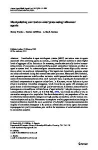
Table 2 Summary of all methods presented to segment OARs in brain cancer.

Contrary to statistical models, DM provide flexibility and do not require explicit training, though they are sensitive to initialization and noise. SMs may lead to greater robustness, however they are more rigid than DM and 580

may be over-constrained, not generalizing well to the unsampled population, particularly for small amounts of training data relative to the dimensionality. This situation can appear on new input examples with pathologies, lesions or presenting high variance, different from the training set. Models having local priors similar to DM formulation do not have this problem. They will easily

585

deform to highly complex shapes found in the unseen image. Hence, many methods attempt to find a balance between the flexibility of the DM and the strict shape constraints of the SM by fusing learnt shape constraints with the deformable model. Notwithstanding, some main limitations have to be taken into account when

590

working with generic parametric DM. First, if the stopping criterion is not defined properly, or boundaries of the structures are noisy, DM may get stuck in a local minimum which does not correspond to the desired boundary. Second, in situations where the initial model and the desired object boundary differ greatly in size and shape, the model must be reparameterized dynamically to faithfully

595

recover the object boundary. Methods for reparameterization in 2D are usually straightforward and require moderate computational overhead. However, reparameterization in 3D requires complicated and computationally expensive methods. Further, it has difficulties when dealing with topological adaptation, caused by the fact that a new parameterization must be constructed whenever

600

the topology change occurs, which may require sophisticated schemes. This issue can be overcome by using Level sets. Moreover, as DM represent a local search, they must be initialized near the structure of interest. By introducing machine learning methods, algorithms developed for medical image processing often become more intelligent than conventional techniques.

605

Improvements in the resulting relative overlaps came from the application of the machine learning methods including ANN and SVM[57]. A comparison done in this work between four methods (template based, probabilistic atlas, 23

ANN and SVM) showed that machine learning algorithms outperformed the template and probabilistic-based methods when comparing the relative overlap. 610

There was also little disparity between the ANN and SVM based segmentation algorithms. ANN training took significantly longer than SVM training but can be applied more quickly to segment the regions of interest. It was reported that it took a day to train an ANN for the classification of only one structure from the others even though a random sampled data was used instead of the whole

615

dataset. While machine learning methods are undoubtedly powerful tools for classification and pattern recognition, there are potential disadvantages when applying them to a given problem. Machine learning approaches, in general, are notoriously hard to interpret and analyze, and in situations where it is desirable to simply and concisely define the process transforming inputs to output values

620

it can be difficult to justify their use. However, despite the large number of presented techniques to perform automatic segmentation of brain subcortical structures, it still remains challenging, especially when lesions, such as tumors, are present. The presence of lesions in the brain might compress some of the subcortical areas, making these de-

625

formations hard to model by some of the presented methods. Thus, the main challenge lies in the segmentation of subcortical structures with anatomical deviation caused by the presence of tumor with different shape, size, location and intensities. The tumor not only changes the part of the brain where tumor exists, but also sometimes influences shape and intensities of other structures of

630

the brain. Thus the existence of such anatomical deviation makes use of prior information about intensity and spatial distribution challenging.

7. Conclusion Four approaches applicable to the (semi-)automatic segmentation of subcortical brain structures in general have been presented in this work. In spite of 635

the availability of a large variety of state-of-art methods for subcortical brain structures segmentation on MRI, we may conclude that there is a gap missing

24

in such state-of-the-art, as no subcortical structures segmentation methods with presence of tumors seem to have been fully explored yet. The development of segmentation algorithms that can deal with such lesions 640

in the brain and still provide a good performance when segmenting subcortical structures is highly required in practice by some clinical applications, such as radiotherapy or radio-surgery.

References [1] R. Siegel, J. Ma, Z. Zou, A. Jemal, Cancer statistics, 2014, CA: a cancer 645

journal for clinicians 64 (1) (2014) 9–29. [2] G. A. Whitfield, P. Price, G. J. Price, C. J. Moore, Automated delineation of radiotherapy volumes: are we going in the right direction?, The British journal of radiology 86 (1021) (2013) 20110718–20110718. [3] P.-Y. Bondiau, G. Malandain, S. Chanalet, P.-Y. Marcy, J.-L. Habrand,

650

F. Fauchon, P. Paquis, A. Courdi, O. Commowick, I. Rutten, et al., Atlas-based automatic segmentation of mr images: validation study on the brainstem in radiotherapy context, International Journal of Radiation Oncology* Biology* Physics 61 (1) (2005) 289–298. [4] M. Yamamoto, Y. Nagata, K. Okajima, T. Ishigaki, R. Murata, T. Mi-

655

zowaki, M. Kokubo, M. Hiraoka, Differences in target outline delineation from ct scans of brain tumours using different methods and different observers, Radiotherapy and oncology 50 (2) (1999) 151–156. [5] J. Grimm, T. LaCouture, R. Croce, I. Yeo, Y. Zhu, J. Xue, Dose tolerance limits and dose volume histogram evaluation for stereotactic body

660

radiotherapy, Journal of Applied Clinical Medical Physics 12 (2). [6] M. A. Hunt, M. J. Zelefsky, S. Wolden, C.-S. Chui, T. LoSasso, K. Rosenzweig, L. Chong, S. V. Spirou, L. Fromme, M. Lumley, et al., Treatment

25

planning and delivery of intensity-modulated radiation therapy for primary nasopharynx cancer, International Journal of Radiation Oncology* 665

Biology* Physics 49 (3) (2001) 623–632. [7] R. D. Timmerman, An overview of hypofractionation and introduction to this issue of¡ i¿ seminars in radiation oncology¡/i¿, in: Seminars in radiation oncology, Vol. 18, WB Saunders, 2008, pp. 215–222. [8] M. S. Sharma, D. Kondziolka, A. Khan, H. Kano, A. Niranjan, J. C.

670

Flickinger, L. D. Lunsford, Radiation tolerance limits of the brainstem, Neurosurgery 63 (4) (2008) 728–733. [9] A. Narayana, J. Yamada, S. Berry, P. Shah, M. Hunt, P. H. Gutin, S. A. Leibel, Intensity-modulated radiotherapy in high-grade gliomas: clinical and dosimetric results, International Journal of Radiation Oncology* Bi-

675

ology* Physics 64 (3) (2006) 892–897. [10] R. F. Mould, Robotic radiosurgery, CyberKnife Society Press, 2005. [11] N. Bhandare, A. Jackson, A. Eisbruch, C. C. Pan, J. C. Flickinger, P. Antonelli, W. M. Mendenhall, Radiation therapy and hearing loss, International journal of radiation oncology, biology, physics 76 (3 Suppl) (2010)

680

S50. [12] N. Massager, O. Nissim, C. Delbrouck, I. Delpierre, D. Devriendt, F. Desmedt, D. Wikler, J. Brotchi, M. Levivier, Irradiation of cochlear structures during vestibular schwannoma radiosurgery and associated hearing outcome.

685

[13] P. Romanelli, A. Muacevic, S. Striano, Radiosurgery for hypothalamic hamartomas. [14] M. Lee, M. Y. S. Kalani, S. Cheshier, I. C. Gibbs, J. R. Adler Jr, S. D. Chang, Radiation therapy and cyberknife radiosurgery in the management of craniopharyngiomas.

26

690

[15] S. L. Stafford, B. E. Pollock, J. A. Leavitt, R. L. Foote, P. D. Brown, M. J. Link, D. A. Gorman, P. J. Schomberg, A study on the radiation tolerance of the optic nerves and chiasm after stereotactic radiosurgery, International Journal of Radiation Oncology* Biology* Physics 55 (5) (2003) 1177–1181.

695

[16] J. Xuan, T. Adali, Y. Wang, Segmentation of magnetic resonance brain image: integrating region growing and edge detection, in: Image Processing, 1995. Proceedings., International Conference on, Vol. 3, IEEE, 1995, pp. 544–547. [17] N. Senthilkumaran, R. Rajesh, Brain image segmentation, International

700

Journal of Wisdom Based Computing 1 (3) (2011) 14–18. [18] C.-H. Lee, M. Schmidt, A. Murtha, A. Bistritz, J. Sander, R. Greiner, Segmenting brain tumors with conditional random fields and support vector machines, in: Computer vision for biomedical image applications, Springer, 2005, pp. 469–478.

705

[19] K. A. Norman, How hippocampus and cortex contribute to recognition memory: revisiting the complementary learning systems model, Hippocampus 20 (11) (2010) 1217–1227. [20] M. Laakso, K. Partanen, P. Riekkinen, M. Lehtovirta, E.-L. Helkala, M. Hallikainen, T. Hanninen, P. Vainio, H. Soininen, Hippocampal vol-

710

umes in alzheimer’s disease, parkinson’s disease with and without dementia, and in vascular dementia an mri study, Neurology 46 (3) (1996) 678–681. [21] D. Shen, S. Moffat, S. M. Resnick, C. Davatzikos, Measuring size and shape of the hippocampus in mr images using a deformable shape model,

715

Neuroimage 15 (2) (2002) 422–434. [22] R. Hult, Grey-level morphology combined with an artificial neural networks approach for multimodal segmentation of the hippocampus, in: Im27

age Analysis and Processing, 2003. Proceedings. 12th International Conference on, IEEE, 2003, pp. 277–282. 720

[23] S. Hu, P. Coup´e, J. C. Pruessner, D. L. Collins, Appearance-based modeling for segmentation of hippocampus and amygdala using multi-contrast mr imaging, NeuroImage 58 (2) (2011) 549–559. [24] S. Zhao, D. Zhang, X. Song, W. Tan, Segmentation of hippocampus in mri images based on the improved level set, in: Computational Intelligence

725

and Design (ISCID), 2011 Fourth International Symposium on, Vol. 1, IEEE, 2011, pp. 123–126. [25] K. Kwak, U. Yoon, D.-K. Lee, G. H. Kim, S. W. Seo, D. L. Na, H.-J. Shim, J.-M. Lee, Fully-automated approach to hippocampus segmentation using a graph-cuts algorithm combined with atlas-based segmentation and

730

morphological opening, Magnetic resonance imaging 31 (7) (2013) 1190– 1196. [26] D. Zarpalas, P. Gkontra, P. Daras, N. Maglaveras, Hippocampus segmentation through gradient based reliability maps for local blending of acm energy terms, in: Biomedical Imaging (ISBI), 2013 IEEE 10th Interna-

735

tional Symposium on, IEEE, 2013, pp. 53–56. [27] X. Artaechevarria, A. Munoz-Barrutia, C. Ortiz-de Sol´orzano, Combination strategies in multi-atlas image segmentation: Application to brain mr data, Medical Imaging, IEEE Transactions on 28 (8) (2009) 1266–1277. [28] D. L. Collins, J. C. Pruessner, Towards accurate, automatic segmentation

740

of the hippocampus and amygdala from mri by augmenting animal with a template library and label fusion, Neuroimage 52 (4) (2010) 1355–1366. [29] A. R. Khan, N. Cherbuin, W. Wen, K. J. Anstey, P. Sachdev, M. F. Beg, Optimal weights for local multi-atlas fusion using supervised learning and dynamic information (superdyn): Validation on hippocampus segmenta-

745

tion, NeuroImage 56 (1) (2011) 126–139. 28

[30] M. Kim, G. Wu, W. Li, L. Wang, Y.-D. Son, Z.-H. Cho, D. Shen, Segmenting hippocampus from 7.0 tesla mr images by combining multiple atlases and auto-context models, in: Machine Learning in Medical Imaging, Springer, 2011, pp. 100–108. 750

[31] P. Coup´e, J. V. Manj´on, V. Fonov, J. Pruessner, M. Robles, D. L. Collins, Nonlocal patch-based label fusion for hippocampus segmentation, in: Medical Image Computing and Computer-Assisted Intervention– MICCAI 2010, Springer, 2010, pp. 129–136. [32] H. Wang, J. W. Suh, S. R. Das, J. B. Pluta, C. Craige, P. A. Yushkevich,

755

Multi-atlas segmentation with joint label fusion, Pattern Analysis and Machine Intelligence, IEEE Transactions on 35 (3) (2013) 611–623. [33] M. Jorge Cardoso, K. Leung, M. Modat, S. Keihaninejad, D. Cash, J. Barnes, N. C. Fox, S. Ourselin, Steps: Similarity and truth estimation for propagated segmentations and its application to hippocampal

760

segmentation and brain parcelation, Medical image analysis 17 (6) (2013) 671–684. [34] A. Ghanei, H. Soltanian-Zadeh, J. P. Windham, Segmentation of the hippocampus from brain mri using deformable contours, Computerized Medical Imaging and Graphics 22 (3) (1998) 203–216.

765

[35] J. H. Morra, Z. Tu, L. G. Apostolova, A. E. Green, A. W. Toga, P. M. Thompson, Automatic subcortical segmentation using a contextual model, in:

Medical Image Computing and Computer-Assisted Intervention–

MICCAI 2008, Springer, 2008, pp. 194–201. [36] J. H. Morra, Z. Tu, L. G. Apostolova, A. E. Green, A. W. Toga, P. M. 770

Thompson, Comparison of adaboost and support vector machines for detecting alzheimer’s disease through automated hippocampal segmentation, Medical Imaging, IEEE Transactions on 29 (1) (2010) 30–43.

29

[37] S. Panda, A. J. Asman, M. P. DeLisi, L. A. Mawn, R. L. Galloway, B. A. Landman, Robust optic nerve segmentation on clinically acquired ct, in: 775

SPIE Medical Imaging, International Society for Optics and Photonics, 2014, pp. 90341G–90341G. [38] J.-D. Lee, Y.-x. Tseng, L.-c. Liu, C.-H. Huang, A 2-d automatic segmentation scheme for brainstem and cerebellum regions in brain mr imaging, in: Fuzzy Systems and Knowledge Discovery, 2007. FSKD 2007. Fourth

780

International Conference on, Vol. 4, IEEE, 2007, pp. 270–274. [39] C. McIntosh, G. Hamarneh, Medial-based deformable models in nonconvex shape-spaces for medical image segmentation, Medical Imaging, IEEE Transactions on 31 (1) (2012) 33–50. [40] M. E. Leventon, W. E. L. Grimson, O. Faugeras, Statistical shape influ-

785

ence in geodesic active contours, in: Computer Vision and Pattern Recognition, 2000. Proceedings. IEEE Conference on, Vol. 1, IEEE, 2000, pp. 316–323. [41] J. Dolz, H. A. Kirisli, M. Vermandel, L. Massoptier, Multimodal imaging towards individualized radiotherapy treatments, Vol. 1, 2014, Ch. Subcor-

790

tical structures segmentation on MRI using support vector machines, pp. 24–31. [42] S. Duchesne, J. Pruessner, D. Collins, Appearance-based segmentation of medial temporal lobe structures, Neuroimage 17 (2) (2002) 515–531. [43] S. Hu, P. Coup´e, J. C. Pruessner, D. L. Collins, Nonlocal regularization

795

for active appearance model: Application to medial temporal lobe segmentation, Human brain mapping 35 (2) (2014) 377–395. [44] J. Bailleul, S. Ruan, D. Bloyet, B. Romaniuk, Segmentation of anatomical structures from 3d brain mri using automatically-built statistical shape models, in: Image Processing, 2004. ICIP’04. 2004 International Confer-

800

ence on, Vol. 4, IEEE, 2004, pp. 2741–2744. 30

[45] Z. Tu, K. L. Narr, P. Doll´ar, I. Dinov, P. M. Thompson, A. W. Toga, Brain anatomical structure segmentation by hybrid discriminative/generative models, Medical Imaging, IEEE Transactions on 27 (4) (2008) 495–508. [46] T. F. Cootes, C. Beeston, G. J. Edwards, C. J. Taylor, A unified frame805

work for atlas matching using active appearance models, in: Information Processing in Medical Imaging, Springer, 1999, pp. 322–333. [47] K. O. Babalola, T. F. Cootes, C. J. Twining, V. Petrovic, C. Taylor, 3d brain segmentation using active appearance models and local regressors, in: Medical Image Computing and Computer-Assisted Intervention–

810

MICCAI 2008, Springer, 2008, pp. 401–408. [48] R. A. Heckemann, J. V. Hajnal, P. Aljabar, D. Rueckert, A. Hammers, Automatic anatomical brain mri segmentation combining label propagation and decision fusion, NeuroImage 33 (1) (2006) 115–126. [49] P. Aljabar, R. A. Heckemann, A. Hammers, J. V. Hajnal, D. Rueckert,

815

Multi-atlas based segmentation of brain images: atlas selection and its effect on accuracy, Neuroimage 46 (3) (2009) 726–738. [50] J. M. L¨ otj¨ onen, R. Wolz, J. R. Koikkalainen, L. Thurfjell, G. Waldemar, H. Soininen, D. Rueckert, Fast and robust multi-atlas segmentation of brain magnetic resonance images, Neuroimage 49 (3) (2010) 2352–2365.

820

[51] A. J. Asman, B. A. Landman, Non-local statistical label fusion for multiatlas segmentation, Medical image analysis 17 (2) (2013) 194–208. [52] M. Wu, C. Rosano, P. Lopez-Garcia, C. S. Carter, H. J. Aizenstein, Optimum template selection for atlas-based segmentation, NeuroImage 34 (4) (2007) 1612–1618.

825

[53] G. Sz´ekely, A. Kelemen, C. Brechb¨ uhler, G. Gerig, Segmentation of 3d objects from mri volume data using constrained elastic deformations of flexible fourier surface models, in: Computer Vision, Virtual Reality and Robotics in Medicine, Springer, 1995, pp. 495–505. 31

[54] J. Yang, J. S. Duncan, 3d image segmentation of deformable objects with 830

joint shape-intensity prior models using level sets, Medical Image Analysis 8 (3) (2004) 285–294. [55] A. Tsai, W. Wells, C. Tempany, E. Grimson, A. Willsky, Mutual information in coupled multi-shape model for medical image segmentation, Medical Image Analysis 8 (4) (2004) 429–445.

835

[56] V. A. Magnotta, D. Heckel, N. C. Andreasen, T. Cizadlo, P. W. Corson, J. C. Ehrhardt, W. T. Yuh, Measurement of brain structures with artificial neural networks: Two-and three-dimensional applications 1, Radiology 211 (3) (1999) 781–790. [57] S. Powell, V. A. Magnotta, H. Johnson, V. K. Jammalamadaka, R. Pier-

840

son, N. C. Andreasen, Registration and machine learning-based automated segmentation of subcortical and cerebellar brain structures, Neuroimage 39 (1) (2008) 238–247. [58] R. Pierson, P. W. Corson, L. L. Sears, D. Alicata, V. Magnotta, D. O’Leary, N. C. Andreasen, Manual and semiautomated measurement

845

of cerebellar subregions on mr images, Neuroimage 17 (1) (2002) 61–76. [59] P. Golland, W. E. L. Grimson, M. E. Shenton, R. Kikinis, Detection and analysis of statistical differences in anatomical shape, Medical image analysis 9 (1) (2005) 69–86. [60] M. Cabezas, A. Oliver, X. Llad´o, J. Freixenet, M. Bach Cuadra, A review

850

of atlas-based segmentation for magnetic resonance brain images, Computer methods and programs in biomedicine 104 (3) (2011) e158–e177. [61] D. L. Hill, P. G. Batchelor, M. Holden, D. J. Hawkes, Medical image registration, Physics in medicine and biology 46 (3) (2001) R1. [62] B. Zitova, J. Flusser, Image registration methods: a survey, Image and

855

vision computing 21 (11) (2003) 977–1000.

32

[63] A. W. Toga, P. M. Thompson, The role of image registration in brain mapping, Image and vision computing 19 (1) (2001) 3–24. [64] T. Rohlfing, R. Brandt, R. Menzel, C. R. Maurer Jr, Evaluation of atlas selection strategies for atlas-based image segmentation with application 860

to confocal microscopy images of bee brains, NeuroImage 21 (4) (2004) 1428–1442. [65] X. Han, M. S. Hoogeman, P. C. Levendag, L. S. Hibbard, D. N. Teguh, P. Voet, A. C. Cowen, T. K. Wolf, Atlas-based auto-segmentation of head and neck ct images, in: Medical Image Computing and Computer-Assisted

865

Intervention–MICCAI 2008, Springer, 2008, pp. 434–441. [66] S. K. Warfield, K. H. Zou, W. M. Wells, Simultaneous truth and performance level estimation (staple): an algorithm for the validation of image segmentation, Medical Imaging, IEEE Transactions on 23 (7) (2004) 903– 921.

870

[67] O. Commowick, A. Akhondi-Asl, S. K. Warfield, Estimating a reference standard segmentation with spatially varying performance parameters: Local map staple, Medical Imaging, IEEE Transactions on 31 (8) (2012) 1593–1606. [68] T. Heimann, H.-P. Meinzer, Statistical shape models for 3d medical image

875

segmentation: A review, Medical image analysis 13 (4) (2009) 543–563. [69] T. F. Cootes, C. J. Taylor, D. H. Cooper, J. Graham, Training models of shape from sets of examples, in: BMVC92, Springer, 1992, pp. 9–18. [70] T. F. Cootes, C. J. Taylor, D. H. Cooper, J. Graham, Active shape modelstheir training and application, Computer vision and image understanding

880

61 (1) (1995) 38–59. [71] T. F. Cootes, G. J. Edwards, C. J. Taylor, Active appearance models, IEEE Transactions on pattern analysis and machine intelligence 23 (6) (2001) 681–685. 33

[72] B. van Ginneken, M. de Bruijne, M. Loog, M. A. Viergever, Interactive 885

shape models, in: Medical Imaging 2003, International Society for Optics and Photonics, 2003, pp. 1206–1216. [73] M. Brejl, M. Sonka, Object localization and border detection criteria design in edge-based image segmentation: automated learning from examples, Medical Imaging, IEEE Transactions on 19 (10) (2000) 973–985.

890

[74] A. Pitiot, H. Delingette, P. M. Thompson, N. Ayache, Expert knowledgeguided segmentation system for brain mri, NeuroImage 23 (2004) S85–S96. [75] Z. Zhao, S. R. Aylward, E. K. Teoh, A novel 3d partitioned active shape model for segmentation of brain mr images, in: Medical Image Computing and Computer-Assisted Intervention–MICCAI 2005, Springer, 2005, pp.

895

221–228. [76] A. Rao, P. Aljabar, D. Rueckert, Hierarchical statistical shape analysis and prediction of sub-cortical brain structures, Medical image analysis 12 (1) (2008) 55–68. [77] F. Bernard, P. Gemmar, A. Husch, F. Hertel, Improvements on the fea-

900

sibility of active shape model-based subthalamic nucleus segmentation, Biomedical Engineering/Biomedizinische Technik. [78] J. Olveres, R. Nava, B. Escalante-Ram´ırez, G. Crist´obal, C. M. Garc´ıaMoreno, Midbrain volume segmentation using active shape models and lbps, in: SPIE Optical Engineering+ Applications, International Society

905

for Optics and Photonics, 2013, pp. 88561F–88561F. [79] E. Adiva, Y. S. Izmantoko, H.-K. Choi, Comparison of active contour and active shape approaches for corpus callosum segmentation 16 (9) (2013) 1018–1030. [80] J. Koikkalainen, T. Tolli, K. Lauerma, K. Antila, E. Mattila, M. Lilja,

910

J. Lotjonen, Methods of artificial enlargement of the training set for sta-

34

tistical shape models, Medical Imaging, IEEE Transactions on 27 (11) (2008) 1643–1654. [81] K. Babalola, T. Cootes, Using parts and geometry models to initialise active appearance models for automated segmentation of 3d medical images, 915

in: Biomedical Imaging: From Nano to Macro, 2010 IEEE International Symposium on, IEEE, 2010, pp. 1069–1072. [82] B. Patenaude, S. M. Smith, D. N. Kennedy, M. Jenkinson, A bayesian model of shape and appearance for subcortical brain segmentation, Neuroimage 56 (3) (2011) 907–922.

920

[83] U. Bagci, X. Chen, J. K. Udupa, Hierarchical scale-based multiobject recognition of 3-d anatomical structures, Medical Imaging, IEEE Transactions on 31 (3) (2012) 777–789. [84] D. Terzopoulos, K. Fleischer, Deformable models, The visual computer 4 (6) (1988) 306–331.

925

[85] L. He, Z. Peng, B. Everding, X. Wang, C. Y. Han, K. L. Weiss, W. G. Wee, A comparative study of deformable contour methods on medical image segmentation, Image and Vision Computing 26 (2) (2008) 141–163. [86] M. Kass, A. Witkin, D. Terzopoulos, Snakes: Active contour models, International journal of computer vision 1 (4) (1988) 321–331.

930

[87] T. McInerney, D. Terzopoulos, T-snakes: Topology adaptive snakes, Medical image analysis 4 (2) (2000) 73–91. [88] S. Osher, J. A. Sethian, Fronts propagating with curvature-dependent speed: algorithms based on hamilton-jacobi formulations, Journal of computational physics 79 (1) (1988) 12–49.

935

[89] Y. Wang, L. H. Staib, Boundary finding with correspondence using statistical shape models, in: Computer Vision and Pattern Recognition, 1998.

35

Proceedings. 1998 IEEE Computer Society Conference on, IEEE, 1998, pp. 338–345. [90] J. S. Duncan, X. Papademetris, J. Yang, M. Jackowski, X. Zeng, L. H. 940

Staib, Geometric strategies for neuroanatomic analysis from mri, Neuroimage 23 (2004) S34–S45. [91] G. Bekes, E. M´ at´e, L. G. Ny´ ul, A. Kuba, M. Fidrich, Geometrical modelbased segmentation of the organs of sight on ct images, Medical physics 35 (2) (2008) 735–743.

945

[92] M. Lee, W. Cho, S. Kim, S. Park, J. H. Kim, Segmentation of interest region in medical volume images using geometric deformable model, Computers in biology and medicine 42 (5) (2012) 523–537. [93] R. Spinks, V. A. Magnotta, N. C. Andreasen, K. C. Albright, S. Ziebell, P. Nopoulos, M. Cassell, Manual and automated measurement of the

950

whole thalamus and mediodorsal nucleus using magnetic resonance imaging, Neuroimage 17 (2) (2002) 631–642. [94] M. J. Moghaddam, H. Soltanian-Zadeh, Automatic segmentation of brain structures using geometric moment invariants and artificial neural networks, in: Information Processing in Medical Imaging, Springer, 2009,

955

pp. 326–337. [95] A. Akselrod-Ballin, M. Galun, M. J. Gomori, R. Basri, A. Brandt, Atlas guided identification of brain structures by combining 3d segmentation and svm classification, in: Medical Image Computing and ComputerAssisted Intervention–MICCAI 2006, Springer, 2006, pp. 209–216.

960

[96] J. Zhou, K. Chan, V. Chong, S. Krishnan, Extraction of brain tumor from mr images using one-class support vector machine, in: Engineering in Medicine and Biology Society, 2005. IEEE-EMBS 2005. 27th Annual International Conference of the, IEEE, 2006, pp. 6411–6414.

36

[97] S. Bauer, L.-P. Nolte, M. Reyes, Fully automatic segmentation of brain 965

tumor images using support vector machine classification in combination with hierarchical conditional random field regularization, in: Medical Image Computing and Computer-Assisted Intervention–MICCAI 2011, Springer, 2011, pp. 354–361. [98] K. Gasmi, A. Kharrat, M. B. Messaoud, M. Abid, Automated segmen-

970

tation of brain tumor using optimal texture features and support vector machine classifier, in: Image Analysis and Recognition, Springer, 2012, pp. 230–239. [99] D. Glotsos, J. Tohka, P. Ravazoula, D. Cavouras, G. Nikiforidis, Automated diagnosis of brain tumours astrocytomas using probabilistic neural

975

network clustering and support vector machines, International journal of neural systems 15 (01n02) (2005) 1–11. [100] C. J. Burges, A tutorial on support vector machines for pattern recognition, Data mining and knowledge discovery 2 (2) (1998) 121–167.

37