common experience of segmentation is the way that an image can resolve itself ..... means to produce the images at center and on the right. We have replaced ...
Chapter 16
SEGMENTATION USING CLUSTERING METHODS
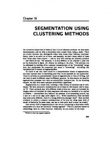
An attractive broad view of vision is that it is an inference problem: we have some measurements, and we wish to determine what caused them, using a mode. There are crucial features that distinguish vision from many other inference problems: firstly, there is an awful lot of data, and secondly, we don’t know which of these data items come from objects — and so help with solving the inference problem — and which do not. For example, it is very difficult to tell whether a pixel lies on the dalmation in figure 16.1 simply by looking at the pixel. This problem can be addressed by working with a compact representation of the “interesting” image data that emphasizes the properties that make it “interesting”. Obtaining this representation is known as segmentation. It’s hard to see that there could be a comprehensive theory of segmentation, not least because what is interesting and what is not depends on the application. There is certainly no comprehensive theory of segmentation at time of writing, and the term is used in different ways in different quarters. In this chapter we describe segmentation processes that have no probabilistic interpretation. In the following chapter, we deal with more complex probabilistic algorithms. Segmentation is a broad term, covering a wide variety of problems and of techniques. We have collected a representative set of ideas in this chapter and in chapter ??. These methods deal with different kinds of data set: some are intended for images, some are intended for video sequences and some are intended to be applied to tokens — placeholders that indicate the presence of an interesting pattern, say a spot or a dot or an edge point (figure 16.1). While superficially these methods may seem quite different, there is a strong similarity amongst them1 . Each method attempts to obtain a compact representation of its data set using some form of model of similarity (in some cases, one has to look quite hard to spot the model). One natural view of segmentation is that we are attempting to determine which components of a data set naturally “belong together”. This is a problem known as clustering; there is a wide literature. Generally, we can cluster in two ways: 1 Which
is why they appear together!
433
434
Segmentation using Clustering Methods
Chapter 16
Figure 16.1. As the image of a dalmation on a shadowed background indicates, an important component of vision involves organising image information into meaningful assemblies. The human vision system seems to be able to do so surprisingly well. The blobs that form the dalmation appear to be assembled “because they form a dalmation,” hardly a satisfactory explanation, and one that begs difficult computational questions. This process of organisation can be applied to many different kinds of input. figure from Marr, Vision, page101, in the fervent hope that permission will be granted
• Partitioning: here we have a large data set, and carve it up according to some notion of the association between items inside the set. We would like to decompose it into pieces that are “good” according to our model. For example, we might: – decompose an image into regions which have coherent colour and texture inside them; – take a video sequence and decompose it into shots — segments of video showing about the same stuff from about the same viewpoint; – decompose a video sequence into motion blobs, consisting of regions that have coherent colour, texture and motion. • Grouping: here we have a set of distinct data items, and wish to collect sets of data items that “make sense” together according to our model. Effects like
Section 16.1.
Human vision: Grouping and Gestalt
435
occlusion mean that image components that belong to the same object are often separated. Examples of grouping include: – collecting together tokens that, taken together, forming an interesting object (as in collecting the spots in figure 16.1); – collecting together tokens that seem to be moving together .
16.1
Human vision: Grouping and Gestalt
Early psychophysics studied the extent to which a stimulus needed to be changed to obtain a change in response. For example, Webers’ law attempts to capture the relationship between the intensity of a stimulus and its perceived brightness for very simple stimuli. The Gestalt school of psychologists rejected this approach, and emphasized grouping as an important part of understanding human vision. A common experience of segmentation is the way that an image can resolve itself into a figure — typically, the significant, important object — and a ground — the background on which the figure lies. However, as figure 16.2 illustrates, what is figure and what is ground can be profoundly ambiguous, meaning that a richer theory is required.
Figure 16.2. One view of segmentation is that it determines which component of the image forms the figure, and which the ground. The figure on the left illustrates one form of ambiguity that results from this view; the white circle can be seen as figure on the black triangular ground, or as ground where the figure is a black triangle with a circular whole in it — the ground is then a white square. On the right, another ambiguity: if the figure is black, then the image shows a vase, but if it is white, the image shows a pair of faces. figure from Gordon, Theories of Visual Perception, page 65,66 in the fervent hope that permission will be granted The Gestalt school used the notion of a gestalt — a whole or a group — and of its gestaltqualit¨ at — the set of internal relationships that makes it a whole
436
Segmentation using Clustering Methods
Chapter 16
Figure 16.3. The famous Muller-Lyer illusion; the horizontal lines are in fact the same length, though that belonging to the upper figure looks longer. Clearly, this effect arises from some property of the relationships that form the whole (the gestaltqualit¨ at), rather than from properties of each separate segment. figure from Gordon, Theories of Visual Perception, page 71 in the fervent hope that permission will be granted
(e.g. figure 16.3) as central components in their ideas. Their work was characterised by attempts to write down a series of rules by which image elements would be associated together and interpreted as a group. There were also attempts to construct algorithms, which are of purely historical interest (see [?] for an introductory account that places their work in a broad context). The Gestalt psychologists identified a series of factors, which they felt predisposed a set of elements to be grouped. There are a variety of factors, some of which postdate the main Gestalt movement: • Proximity: tokens that are nearby tend to be grouped. • Similarity: similar tokens tend to be grouped together. • Common fate: tokens that have coherent motion tend to be grouped together. • Common region: tokens that lie inside the same closed region tend to be grouped together. • Parallelism: parallel curves or tokens tend to be grouped together. • Closure: tokens or curves that tend to lead to closed curves tend to be grouped together. • Symmetry: curves that lead to symmetric groups are grouped together. • Continuity: tokens that lead to “continuous” — as in “joining up nicely”, rather than in the formal sense — curves tend to be grouped. • Familiar Configuration: tokens that, when grouped, lead to a familiar object, tend to be grouped together — familiar configuration can be seen as the reason that the tokens of figure 16.1 are all collected into a dalmation and a tree.
Section 16.1.
437
Human vision: Grouping and Gestalt
Parallelism Not grouped Proximity
Symmetry
Similarity Similarity Common Fate
Common Region
Continuity
Closure
Figure 16.4. Examples of Gestalt factors that lead to grouping (which are described in greater detail in the text). figure from Gordon, Theories of Visual Perception, page 67 in the fervent hope that permission will be granted
These rules can function fairly well as explanations, but they are insufficiently crisp to be regarded as forming an algorithm. The Gestalt psychologists had serious difficulty with the details, such as when one rule applied and when another. It is very difficult to supply a satisfactory algorithm for using these rules — the Gestalt movement attempted to use an extremality principle. Familiar configuration is a particular problem. The key issue is to understand just what familiar configuration applies in a problem, and how it is selected. For example, look at figure 16.1; one might argue that the blobs are grouped because they yield a dog. The difficulty with this view is explaining how this occurred — where did the hypothesis that a dog is present come from? a search through all views of all objects is one explanation, but one must then explain how this search is organised — do we check every view of every dog with every pattern of spots? how can this be done efficiently? The Gestalt rules do offer some insight, because they offer some explanation for what happens in various examples. These explanations seem to be sensible, because they suggest that the rules help solve problems posed by visual effects that arise commonly in the real world — that is, they are ecologically valid. For example, continuity may represent a solution to problems posed by occlusion — sections of the contour of an occluded object could be joined up by continuity (see figures ??
438
Segmentation using Clustering Methods
Chapter 16
Figure 16.5. Occlusion appears to be an important cue in grouping. With some effort, the pattern on the left can be seen as a cube, whereas the pattern on the right is clearly and immediately a cube. The visual system appears to be helped by evidence that separated tokens are separated for a reason, rather than just scattered. figure from Gordon, Theories of Visual Perception, page 87 in the fervent hope that permission will be granted and 16.5). This tendency to prefer interpretations that are explained by occlusion leads to interesting effects. One is the illusory contour, illustrated in figure 16.6. Here a set of tokens suggests the presence of an object most of whose contour has no contrast. The tokens appear to be grouped together because they provide a cue to the presence of an occluding object, which is so strongly suggested by these tokens that one could fill in the no-contrast regions of contour.
Figure 16.6. The tokens in these images suggest the presence of occluding triangles, whose boundaries don’t contrast with much of the image, except at their vertices. Notice that one has a clear impression of the position of the entire contour of the occluding figures. These contours are known as illusory contours. figure from Marr, Vision, page51, in the fervent hope that permission will be granted This ecological argument has some force, because it is possible to interpret most grouping factors using it. Common fate can be seen as a consequence of the fact that components of objects tend to move together. Equally, symmetry is a useful grouping cue because there are a lot of real objects that have symmetric or close
Section 16.2.
Application: Shot Boundary Detection and Background Subtraction
439
to symmetric contours. Essentially, the ecological argument says that tokens are grouped because doing so produces representations that are helpful for the visual world that people encounter. The ecological argument has an appealing, though vague, statistical flavour. From our perspective, Gestalt factors provide interesting hints, but should be seen as the consequences of a larger grouping process, rather than the process itself.
16.2
Application: Shot Boundary Detection and Background Subtraction
Simple segmentation algorithms are often very useful in significant applications. Generally, simple algorithms work best when it is very easy to tell what a “useful” decomposition is. Two important cases are background subtraction — where anything that doesn’t look like a known background is interesting — and shot boundary detection — where substantial changes in a video are interesting.
16.2.1
Background Subtraction
In many applications, objects appear on a background which is very largely stable. The standard example is detecting parts on a conveyor belt. Another example is counting motor cars in an overhead view of a road — the road itself is pretty stable in appearance. Another, less obvious, example is in human computer interaction. Quite commonly, a camera is fixed (say, on top of a monitor) and views a room. Pretty much anything in the view that doesn’t look like the room is interesting. In these kinds of applications, a useful segmentation can often be obtained by subtracting an estimate of the appearance of the background from the image, and looking for large absolute values in the result. The main issue is obtaining a good estimate of the background. One method is simply to take a picture. This approach works rather poorly, because the background typically changes slowly over time. For example, the road may get more shiny as it rains and less when the weather dries up; people may move books and furniture around in the room, etc. An alternative which usually works quite well is to estimate the value of background pixels using a moving average. In this approach, we estimate the value of a particular background pixel as a weighted average of the previous values. Typically, pixels in the very distant past should be weighted at zero, and the weights increase smoothly. Ideally, the moving average should track the changes in the background, meaning that if the weather changes very quickly (or the book mover is frenetic) relatively few pixels should have non-zero weights, and if changes are slow, the number of past pixels with non-zero weights should increase. This yields algorithm 1 For those who have read the filters chapter, this is a filter that smooths a function of time, and we would like it to suppress frequencies that are larger than the typical frequency of change in the background and pass those that are at or below that frequency. As figures 16.7 and 16.8 indicate, the approach can be quite successful.
440
Segmentation using Clustering Methods
Chapter 16
Form a background estimate B(0) . At each frame F Update the background�estimate, typically by wa F + wi B (n−i) i forming B(n+1) = wc for a choice of weights wa , wi and wc . Subtract the background estimate from the frame, and report the value of each pixel where the magnitude of the difference is greater than some threshold. end 16.1: Background Subtraction
Figure 16.7. Moving average results for human segmentation
Figure 16.8. Moving average results for car segmentation
Algorithm
Section 16.2.
16.2.2
Application: Shot Boundary Detection and Background Subtraction
441
Shot Boundary Detection
Long sequences of video are composed of shots — much shorter subsequences that show largely the same objects. These shots are typically the product of the editing process. There is seldom any record of where the boundaries between shots fall. It is helpful to represent a video as a collection of shots; each shot can then be represented with a key frame. This representation can be used to search for videos or to encapsulate their content for a user to browse a video or a set of videos. Finding the boundaries of these shots automatically — shot boundary detection — is an important practical application of simple segmentation algorithms. A shot boundary detection algorithm must find frames in the video that are “significantly” different from the previous frame. Our test of significance must take account of the fact that within a given shot both objects and the background can move around in the field of view. Typically, this test takes the form of a distance; if the distance is larger than a threshold, a shot boundary is declared (algorithm 2).
For each frame in an image sequence Compute a distance between this frame and the previous frame If the distance is larger than some threshold,
Algorithm 16.2:
classify the frame as a shot boundary. end Shot boundary detection using interframe differences There are a variety of standard techniques for computing a distance: • Frame differencing algorithms take pixel-by-pixel differences between each two frames in a sequence, and sum the squares of the differences. These algorithms are unpopular, because they are slow — there are many differences — and because they tend to find many shots when the camera is shaking. • Histogram based algorithms compute colour histograms for each frame, and compute a distance between the histograms. A difference in colour histograms is a sensible measure to use, because it is insensitive to the spatial arrangement of colours in the frame — for example, small camera jitters will not affect the histogram. • Block comparison algorithms compare frames by cutting them into a grid of boxes, and comparing the boxes. This is to avoid the difficulty with colour
442
Segmentation using Clustering Methods
Chapter 16
Figure 16.9. Shot boundary detection results. histograms, where (for example) a red object disappearing off-screen in the bottom left corner is equivalent to a red object appearing on screen from the top edge. Typically, these block comparison algorithms compute an interframe distance that is a composite — taking the maximum is one natural strategy — of inter-block distances, computed using the methods above. • Edge differencing algorithms compute edge maps for each frame, and then compare these edge maps. Typically, the comparison is obtained by counting the number of potentially corresponding edges (nearby, similar orientation, etc.) in the next frame. If there are few potentially corresponding edges, there is a shot boundary. A distance can be obtained by transforming the number of corresponding edges. These are relatively ad hoc methods, but are often sufficient to solve the problem at hand.
16.3
Image Segmentation by Clustering Pixels
Clustering is a process whereby a data set is replaced by clusters, which are collections of data points that “belong together”. It is natural to think of image segmentation as clustering; we would like to represent an image in terms of clusters of pixels that “belong together”. The specific criterion to be used depends on the application. Pixels may belong together because they have the same colour and/or they have the same texture and/or they are nearby, etc.
16.3.1
Simple Clustering Methods
There are two natural algorithms for clustering. In divisive clustering, the entire data set is regarded as a cluster, and then clusters are recursively split to yield a good clustering (algorithm 4). In agglomerative clustering, each data item is regarded as a cluster and clusters are recursively merged to yield a good clustering (algorithm 3).
Section 16.3.
443
Image Segmentation by Clustering Pixels
Make each point a separate cluster Until the clustering is satisfactory Merge the two clusters with the smallest inter-cluster distance
Algorithm 16.3:
Agglomerative
end clustering, or clustering by merging
Construct a single cluster containing all points Until the clustering is satisfactory Split the cluster that yields the two components with the largest inter-cluster distance
Algorithm
end 16.4: Divisive clustering, or clustering by splitting There are two major issues in thinking about clustering: • what is a good inter-cluster distance? Agglomerative clustering uses an intercluster distance to fuse “nearby” clusters; divisive clustering uses it to split insufficiently “coherent” clusters. Even if a natural distance between data points is available (which may not be the case for vision problems), there is no canonical inter-cluster distance. Generally, one chooses a distance that seems appropriate for the data set. For example, one might choose the distance between the closest elements as the inter-cluster distance — this tends to yield extended clusters (statisticians call this method single-link clustering). Another natural choice is the maximum distance between an element of the first cluster and one of the second — this tends to yield “rounded” clusters (statisticians call this method complete-link clustering). Finally, one could use an average of distances between elements in the clusters — this will also tend to yield “rounded” clusters (statisticians call this method group average clustering). • and how many clusters are there? This is an intrinsically difficult task if there is no model for the process that generated the clusters. The algorithms
444
Segmentation using Clustering Methods
Chapter 16
distance
we have described generate a hierarchy of clusters. Usually, this hierarchy is displayed to a user in the form of a dendrogram — a representation of the structure of the hierarchy of clusters that displays inter-cluster distances — and an appropriate choice of clusters is made from the dendrogram (see the example in figure 16.10).
6 5 4
1 2 3
1 2 3 4 5 6 Figure 16.10. Left, a data set; right, a dendrogram obtained by agglomerative clustering using single link clustering. If one selects a particular value of distance, then a horizontal line at that distance will split the dendrogram into clusters. This representation makes it possible to guess how many clusters there are, and to get some insight into how good the clusters are.
16.3.2
Segmentation Using Simple Clustering Methods
It is relatively easy to take a clustering method and build an image segmenter from it. Much of the literature on image segmentation consists of papers that are, in essence, papers about clustering (though this isn’t always acknowledged). The distance used depends entirely on the application, but measures of colour difference and of texture are commonly used as clustering distances. It is often desirable to have clusters that are “blobby”; this can be achieved by using difference in position in the clustering distance. The main difficulty in using either agglomerative or divisive clustering methods directly is that there are an awful lot of pixels in an image. There is no reasonable prospect of examining a dendrogram, because the quantity of data means that
Section 16.3.
Image Segmentation by Clustering Pixels
445
Figure 16.11. We illustrate an early segmenter that uses a divisive clustering algorithm, due to [?] (circa 1975) using this figure of a house, which is segmented into the hierarchy of regions indicated in figure 16.12.
it will be too big. Furthermore, the mechanism is suspect; we don’t really want to look at a dendrogram for each image, but would rather have the segmenter produce useful regions for an application on a long sequence of images without any help. In practice, this means that the segmenters decide when to stop splitting or merging by using a set of threshold tests — for example, an agglomerative segmenter may stop merging when the distance between clusters is sufficiently low, or when the number of clusters reaches some value. The choice of thresholds is usually made by observing the behaviour of the segmenter on a variety of images, and choosing the best setting. The technique has largely fallen into disuse except in specialised applications, because in most cases it is very difficult to predict the future performance of the segmenter tuned in this way. Another difficulty created by the number of pixels is that it is impractical to look for the best split of a cluster (for a divisive method) or the best merge (for an agglomerative method). The variety of tricks that have been adopted to address this problem is far too large to survey here, but we can give an outline of the main strategies. Divisive methods are usually modified by using some form of summary of a cluster to suggest a good split. A natural summary to use is a histogram of pixel colours (or grey levels). In one of the earliest segmentation algorithms, due to Ohlander [?], regions are split by identifying a peak in one of nine feature histograms (these are colour coordinates of the pixel in each of three different colour spaces) and attempting to separate that peak from the histogram. Of course, textured regions
446
Segmentation using Clustering Methods
Chapter 16
Figure 16.12. The hierarchy of regions obtained from figure 16.11, by a divisive clustering algorithm. A typical histogram is shown in figure 16.13. The segmentation process is stopped when regions satisfy an internal coherence test, defined by a collection of fixed thresholds. need to be masked to avoid splitting texture components apart. Figures 16.12 and 16.13 illustrate this segmenter. Agglomerative methods also need to be modified. There are three main issues: • Firstly, given two clusters containing large numbers of pixels, it is expensive to find the average distance or the minimum distance between elements of the clusters; alternatives include the distance between centers of gravity. • Secondly, it is usual to try and merge only clusters with shared boundaries (this can be accounted for by attaching a term to the distance function that is zero for neighbouring pixels and infinite for all others). This approach avoids clustering together regions that are widely separated (we probably don’t wish to represent the US flag as three clusters, one red, one white and one blue). • Finally, it can be useful to merge regions simply by scanning the image and
Section 16.3.
Image Segmentation by Clustering Pixels
447
Figure 16.13. A histogram encountered while segmenting figure 16.11 into the hierarchy of figure 16.12 using the divisive clustering algorithm of [?].
merging all pairs whose distance falls below a threshold, rather than searching for the closest pair. This strategy means the dendrogram is meaningless, but the dendrogram is so seldom used this doesn’t usually matter.
16.3.3
Clustering and Segmentation by K-means
Simple clustering methods use greedy interactions with existing clusters to come up with a good overall representation. For example, in agglomerative clustering we repeatedly make the best available merge. However, the methods are not explicit about the objective function that the methods are attempting to optimize. An alternative approach is to write down an objective function that expresses how good a representation is, and then build an algorithm for obtaining the best representation. A natural objective function can be obtained by assuming that we know there are k clusters, where k is known. Each cluster is assumed to have a center; we write the center of the i’th cluster as ci . The j’th element to be clustered is described by a feature vector xj . For example, if we were segmenting scattered points, then x would be the coordinates of the points; if we were segmenting an intensity image, x might be the intensity at a pixel. We now assume that elements are close to the center of their cluster, yielding the objective function � � Φ(clusters, data) = (xj − ci )T (xj − ci ) i∈clusters j∈i‘th cluster Notice that if the allocation of points to clusters is known, it is easy to compute the best center for each cluster. However, there are far too many possible allocations of points to clusters to search this space for a minimum. Instead, we define an algorithm which iterates through two activities: • Assume the cluster centers are known, and allocate each point to the closest cluster center.
448
Segmentation using Clustering Methods
Chapter 16
• Assume the allocation is known, and choose a new set of cluster centers. Each center is the mean of the points allocated to that cluster. We then choose a start point by randomly choosing cluster centers, and then iterate these stages alternately. This process will eventually converge to a local minimum of the objective function (why?). It is not guaranteed to converge to the global minimum of the objective function, however. It is also not guaranteed to produce k clusters, unless we modify the allocation phase to ensure that each cluster has some non-zero number of points. This algorithm is usually referred to as k-means. It is possible to search for an appropriate number of clusters by applying k-means for different values of k, and comparing the results; we defer a discussion of this issue until section 18.3. Choose k data points to act as cluster centers Until the cluster centers are unchanged Allocate each data point to cluster whose center is nearest Now ensure that one data point; supplying empty points far from
every cluster has at least possible techniques for doing this include . clusters with a point chosen at random from their cluster center.
Replace the cluster centers with the mean of the elements in their clusters. end Algorithm 16.5: Clustering by K-Means One difficulty with using this approach for segmenting images is that segments are not connected and can be scattered very widely (figures 16.14 and 16.15). This effect can be reduced by using pixel coordinates as features, an approach that tends to result in large regions being broken up (figure 16.16).
16.4
Segmentation by Graph-Theoretic Clustering
Clustering can be seen as a problem of cutting graphs into “good” pieces. In effect, we associate each data item with a vertex in a weighted graph, where the weights on the edges between elements are large if the elements are “similar” and small if they are not. We then attempt to cut the graph into connected components with relatively large interior weights — which correspond to clusters — by cutting edges
Section 16.4.
Segmentation by Graph-Theoretic Clustering
449
Figure 16.14. On the left, an image of mixed vegetables, which is segmented using kmeans to produce the images at center and on the right. We have replaced each pixel with the mean value of its cluster; the result is somewhat like an adaptive requantization, as one would expect. In the center, a segmentation obtained using only the intensity information. At the right, a segmentation obtained using colour information. Each segmentation assumes five clusters.
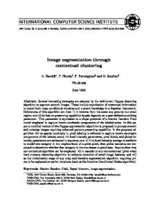
Figure 16.15. Here we show the image of vegetables segmented with k-means, assuming a set of 11 components. The top left figure shows all segments shown together, with the mean value in place of the original image values. The other figures show four of the segments. Note that this approach leads to a set of segments that are not necessarily connected. For this image, some segments are actually quite closely associated with objects but one segment may represent many objects (the peppers); others are largely meaningless. The absence of a texture measure creates serious difficulties, as the many different segments resulting from the slice of red cabbage indicate. with relatively low weights. This view leads to a series of different, quite successful, segmentation algorithms.
16.4.1
Basic Graphs
We review terminology here very briefly, as it’s quite easy to forget. • A graph is a set of vertices V and edges E which connect various pairs of
450
Segmentation using Clustering Methods
Chapter 16
Figure 16.16. Five of the segments obtained by segmenting the image of vegetables with a k-means segmenter that uses position as part of the feature vector describing a pixel, now using 20 segments rather than 11. Note that the large background regions that should be coherent has been broken up because points got too far from the center. The individual peppers are now better separated, but the red cabbage is still broken up because there is no texture measure. vertices. A graph can be written G = {V, E}. Each edge can be represented by a pair of vertices, that is E ⊂ V × V . Graphs are often drawn as a set of points with curves connecting the points. • A directed graph is one in which edges (a, b) and (b, a) are distinct; such a graph is drawn with arrowheads indicating which direction is intended. • An undirected graph is one in which no distinction is drawn between edges (a, b) and (b, a). • A weighted graph is one in which a weight is associated with each edge. • A self-loop is an edge that has the same vertex at each end; self-loops don’t occur in practice in our applications. • Two vertices are said to be connected if there is a sequence of edges starting at the one and ending at the other; if the graph is directed, then the arrows in this sequence must point the right way. • A connected graph is one where every pair of vertices is connected. • Every graph consists of a disjoint set of connected components, that is G = {V1 ∪ V2 . . . Vn , E1 ∪ E2 . . . En }, where {Vi , Ei } are all connected graphs and there is no edge in E that connects an element of Vi with one of Vj for i = j.
16.4.2
The Overall Approach
It is useful to understand that a weighted graph can be represented by a square matrix (figure 16.17). There is a row and a column for each vertex. The i, j’th element of the matrix represents the weight on the edge from vertex i to vertex j;
Section 16.4.
451
Segmentation by Graph-Theoretic Clustering
for an undirected graph, we use a symmetric matrix and place half the weight in each of the i, j’th and j, i’th element.
0.1 2
1 3
2
5 2
2
4 7 1
0.1 1 2 5 2
3 2
2
4 7 1
Figure 16.17. On the top left, a drawing of an undirected weighted graph; on the top right, the weight matrix associated with that graph. Larger values are lighter. By associating the vertices with rows (and columns) in a different order, the matrix can be shuffled. We have chosen the ordering to show the matrix in a form that emphasizes the fact that it is very largely block-diagonal. The figure on the bottom shows a cut of that graph that decomposes the graph into two tightly linked components. This cut decomposes the graph’s matrix into the two main blocks on the diagonal.
The application of graphs to clustering is this: take each element of the collection to be clustered, and associate it with a vertex on a graph. Now construct an edge from every element to every other, and associate with this edge a weight representing the extent to which the elements are similar. Now cut edges in the graph to form a “good” set of connected components. Each of these will be a cluster. For example, figure 16.18 shows a set of well separated points and the weight matrix (i.e. undirected weighted graph, just drawn differently) that results from a particular similarity measure; a desirable algorithm would notice that this matrix looks a lot like a block diagonal matrix — because intercluster similarities are
452
Segmentation using Clustering Methods
Chapter 16
strong and intracluster similarities are weak — and split it into two matrices, each of which is a block. The issues to study are the criteria that lead to good connected components and the algorithms for forming these connected components.
16.4.3
Affinity Measures
When we viewed segmentation as simple clustering, we needed to supply some measure of how similar clusters were. The current model of segmentation simply requires a weight to place on each edge of the graph; these weights are usually called affinity measures in the literature. Clearly, the affinity measure depends on the problem at hand. The weight of an arc connecting similar nodes should be large, and the weight on an arc connecting very different nodes should be small. It is fairly easy to come up with affinity measures with these properties for a variety of important cases, and we can construct an affinity function for a combination of cues by forming a product of powers of these affinity functions. You should be aware that other choices of affinity function are possible; there is no particular reason to believe that a canonical choice exists.
Figure 16.18. On the left, a set of points on the plane. On the right, the affinity matrix for these points computed using a decaying exponential in distance (section 16.4.3), where large values are light and small values are dark. Notice the near block diagonal structure of this matrix; there are two off-diagonal blocks that contain terms that are very close to zero. The blocks correspond to links internal to the two obvious clusters, and the off diagonal blocks correspond to links between these clusters. figure from Perona and Freeman, A factorization approach to grouping, page 2 figure from Perona and Freeman, A factorization approach to grouping, page 4
Affinity by Distance Affinity should go down quite sharply with distance, once the distance is over some threshold. One appropriate expression has the form
� aff(x, y) = exp − (x − y)t (x − y)/2σd2
Section 16.4.
Segmentation by Graph-Theoretic Clustering
453
where σd is a parameter which will be large if quite distant points should be grouped and small if only very nearby points should be grouped (this is the expression used for figure 16.18). Affinity by Intensity Affinity should be large for similar intensities, and smaller as the difference increases. Again, an exponential form suggests itself, and we can use:
� aff(x, y) = exp − (I(x) − I(y))t (I(x) − I(y))/2σI2 Affinity by Colour We need a colour metric to construct a meaningful colour affinity function. It’s a good idea to use a uniform colour space, and a bad idea to use RGB space, — for reasons that should be obvious, otherwise, reread section ?? — and an appropriate expression has the form �
aff(x, y) = exp − dist(c(x), c(y))2 /2σc2 where ci is the colour at pixel i. Affinity by Texture The affinity should be large for similar textures and smaller as the difference increases. We adopt a collection of filters f1 , . . . , fn , and describe textures by the outputs of these filters, which should span a range of scales and orientations. Now for most textures, the filter outputs will not be the same at each point in the texture — think of a chessboard — but a histogram of the filter outputs constructed over a reasonably sized neighbourhood will be well behaved. For example, in the case of an infinite chessboard, if we take a histogram of filter outputs over a region that covers a few squares, we can expect this histogram to be the same wherever the region falls. This suggests a process where we firstly establish a local scale at each point — perhaps by looking at energy in coarse scale filters, or using some other method — and then compute a histogram of filter outputs over a region determined by that scale — perhaps a circular region centered on the point in question. We then write h for this histogram, and use an exponential form:
� aff(x, y) = exp − (f (x) − f (y))t (f (x) − f (y))/2σI2 Affinity by Motion In the case of motion, the nodes of the graph are going to represent a pixel in a particular image in the sequence. It is difficult to estimate the motion at a particular pixel accurately; instead, it makes sense to construct a distribution over
454
Segmentation using Clustering Methods
Chapter 16
1.4
1.2
1
0.8
0.6
0.4
0.2
0
-0.2
-0.4 -0.4
-0.2
0
0.2
0.4
0.6
0.8
1
1.2
1.4
Figure 16.19. The choice of scale for the affinity affects the affinity matrix. The top row shows a dataset, which consists of four groups of 10 points drawn from a rotationally symmetric normal distribution with four different means. The standard deviation in each direction for these points is 0.2. In the second row, affinity matrices computed for this dataset using different values of σd . On the left, σd = 0.1, in the center σd = 0.2 and on the right, σd = 1. For the finest scale, the affinity between all points is rather small; for the next scale, there are four clear blocks in the affinity matrix; and for the coarsest scale, the number of blocks is less obvious.
the possible motions. The quality of motion estimate available depends on what the neighbourhood of the pixel looks like. For example, if the pixel lies on an edge, this motion component parallel to the edge is going to be uncertain but the component perpendicular to the edge is going to be quite well measured. One way to obtain a reasonable estimate of the probability distribution is to compare a translated version of the neighbourhood with the next image; if the two are similar, then the probability of this motion should be relatively high. If we define a similarity measure for an image motion v at a pixel x to be S(v, x; σd) = exp −
1 2σd2
� u∈neighbourhood
2 {It (x + u + v) − It+1 (x + u)}
Section 16.4.
Segmentation by Graph-Theoretic Clustering
455
we have a measure that will be near one for a good value of the motion and near zero for a poor one. This can be massaged into a probability distribution by ensuring that it somes to one, so we have Si (v, x; σd) P (v, x; σd ) = � v Si (v, x; σd ) Now we need to obtain an affinity measure from this. The arcs on the graph will connect pixels that are “nearby” in space and in time. For each pair of pixels, the affinity should be high if the motion pattern around the pixels could look similar, and low otherwise. This suggests using a correlation measure for the affinity � �� � � 1 aff(x, y; σd, σm ) = exp − 2 1 − P (v, x; σd )P (v, x; σd ) 2σm v
16.4.4
Eigenvectors and Segmentation
In the first instance, assume that there are k elements and k clusters. We can represent a cluster by a vector with k components. We will allow elements to be associated with clusters using some continuous weight — we need to be a bit vague about the semantics of these weights, but the intention is that if a component in a particular vector has a small value, then it is weakly associated with the cluster, and if it has a large value, then it is strongly associated with a cluster. Extracting a Single Good Cluster A good cluster is one where elements that are strongly associated with the cluster also have large values in the affinity matrix. Write the matrix representing the element affinities as A, and the vector of weights as w In particular, we can construct an objective function wT Aw This is a sum of terms of the form {association of element i with cluster} × {affinity between i and j} × {association of element j with cluster} We can obtain a cluster by choosing a set of association weights that maximise this objective function. The objective function is useless on its own, because scaling w by λ scales the total association by λ2 . However, we can normalise the weights by requiring that wT w = 1. This suggests maximising wT Aw subject to w T w = 1. The Lagrangian is
� w T Aw + λ wT w − 1
456
Segmentation using Clustering Methods
Chapter 16
0.45
0.4
0.35
0.3
0.25
0.2
0.15
0.1
0.05
0
0
5
10
15
20
25
30
35
40
Figure 16.20. The eigenvector corresponding to the largest eigenvalue of the affinity matrix for the dataset of example 16.19, using σd = 0.2. Notice that most values are small, but some — corresponding to the elements of the main cluster — are large. The sign of the association is not significant, because a scaled eigenvector is still an eigenvector. and differentiation and dropping a factor of two yields Aw = λw meaning that w is an eigenvector of A. This means that we could form a cluster by obtaining the eigenvector with the largest eigenvalue — the cluster weights are the elements of the eigenvector. For problems where reasonable clusters are apparent, we expect that these cluster weights are large for some elements — which belong to the cluster — and nearly zero for others — which do not. In fact, we can get the weights for other clusters from other eigenvectors of A as well. Extracting Weights for a Set of Clusters In the kind of problems we expect to encounter, there are strong association weights between relatively few pairs of elements. For example, if each node is a pixel, the association weights will depend on the difference in colour and/or texture and/or intensity. The association weights between a pixel and its neighbours may be large, but the association weights will die off quickly with distance, because there needs to be more evidence than just similarity of colour to say that two widely separated pixels belong together. As a result, we can reasonably expect to be dealing with clusters that are (a) quite tight and (b) distinct. These properties lead to a fairly characteristic structure in the affinity matrix. In particular, if we relabel the nodes of the graph, then the rows and columns of the matrix A are shuffled. We expect to be dealing with relatively few collections of nodes with large association weights; furthermore, that these collections actually
Section 16.4.
457
Segmentation by Graph-Theoretic Clustering
form a series of relatively coherent, largely disjoint clusters. This means that we could shuffle the rows and columns of M to form a matrix that is roughly blockdiagonal (the blocks being the clusters). Shuffling M simply shuffles the elements of its eigenvectors, so that we can reason about the eigenvectors by thinking about a shuffled version of M (i.e. figure 16.17 is a fair source of insight). The eigenvectors of block-diagonal matrices consist of eigenvectors of the blocks, padded out with zeros. We expect that each block has an eigenvector corresponding to a rather large eigenvalue — corresponding to the cluster — and then a series of small eigenvalues of no particular significance. From this, we expect that, if there are c significant clusters (where c < k), the eigenvectors corresponding to the c largest eigenvalues each represent a cluster.
0.05
0.45
0
0.4
-0.05
0.35
-0.1
0.3
-0.15
0.25
-0.2
0.2
-0.25
0.15
0.05
0
-0.05
-0.1
-0.15
-0.2
-0.25 -0.3
0.1
-0.35
0.05
-0.4
0
-0.45
0
5
10
15
20
25
30
35
40
-0.05
-0.3
-0.35
0
5
10
15
20
25
30
35
40
-0.4
0
5
10
15
20
25
30
35
Figure 16.21. The three eigenvectors corresponding to the next three largest eigenvalues of the affinity matrix for the dataset of example 16.19, using σd = 0.2 (the eigenvector corresponding to the largest eigenvalue is given in figure 16.20). Notice that most values are small, but for (disjoint) sets of elements, the corresponding values are large. This follows from the block structure of the affinity matrix. The sign of the association is not significant, because a scaled eigenvector is still an eigenvector.
This means that each of these eigenvectors is an eigenvector of a block, padded with zeros. In particular, a typical eigenvector will have a small set of large values — corresponding to its block — and a set of near-zero values. We expect that only one of these eigenvectors will have a large value for any given component; all the others will be small (figure 16.21). Thus, we can interpret eigenvectors corresponding to the c largest magnitude eigenvalues as cluster weights for the first c clusters. One can usually quantize the cluster weights to zero or one, to obtain discrete clusters; this is what has happened in the figures. This is a qualitative argument, and there are graphs for which the argument is decidedly suspect. Furthermore, we have been decidedly vague about how to determine c, though our argument suggests that poking around in the spectrum of A might be rewarding — one would hope to find a small set of large eigenvalues, and a large set of small eigenvalues (figure 16.22).
40
458
Segmentation using Clustering Methods
Chapter 16
Construct an affinity matrix Compute the eigenvalues and eigenvectors of the affinity matrix Until there are sufficient clusters Take the eigenvector corresponding to the largest unprocessed eigenvalue; zero all components corresponding to elements that have already been clustered, and threshold the remaining components to determine which element belongs to this cluster, choosing a threshold by clustering the components, or using a threshold fixed in advance. If all elements have been accounted for, there are sufficient clusters end
Algorithm 16.6: Clustering by Graph Eigenvectors 2.5
2
5
25
4
20
3
15
2
10
1
5
0
0
1.5
1
0.5
0
-0.5
-1
0
5
10
15
20
25
30
35
40
-1
0
5
10
15
20
25
30
35
40
-5
0
5
10
15
20
25
30
35
Figure 16.22. The number of clusters is reflected in the eigenvalues of the affinity matrix. The figure shows eigenvalues of the affinity matrices for each of the cases in figure 16.19. On the left, σd = 0.1, in the center σd = 0.2 and on the right, σd = 1. For the finest scale, there are many rather large eigenvalues — this is because the affinity between all points is rather small; for the next scale, there are four eigenvalues rather larger than the rest; and for the coarsest scale, there are only two eigenvalues rather larger than the rest.
16.4.5
Normalised Cuts
The qualitative argument of the previous section is somewhat soft. For example, if the eigenvalues of the blocks are very similar, we could end up with eigenvectors
40
Section 16.4.
459
Segmentation by Graph-Theoretic Clustering
5
1.6
1.4
4 1.2
1
3
0.8
2
0.6
0.4
1 0.2
0
0 -0.2
-0.4 -0.4
-0.2
0
0.2
0.4
0.6
0.8
1
0.25
1.2
-1
1.4
0.25
0
5
10
0.25
15
0.2
0.2
0.2
0.2
0.15
0.15
0.15
0.15
0.1
0.1
0.1
0.1
0.05
0.05
0.05
0.05
0
0
0
0
-0.05
-0.05
-0.05
-0.05
-0.1
-0.1
-0.1
-0.1
-0.15
-0.15
-0.15
-0.15
-0.2
-0.2
-0.2
-0.25
-0.25
-0.25
0
5
10
15
20
25
30
35
40
0
5
10
15
20
25
30
35
40
20
25
30
35
40
0.25
-0.2 -0.25
0
5
10
15
20
25
30
35
40
0
5
10
15
20
25
30
35
Figure 16.23. Eigenvectors of an affinity matrix can be a misleading guide to clusters. The dataset on the top left consists of four copies of the same set of points; this leads to a repeated block structure in the affinity matrix shown in the top center. Each block has the same spectrum, and this results in a spectrum for the affinity matrix that has (roughly) four copies of the same eigenvalue (top right). The bottom row shows the eigenvectors corresponding to the four largest eigenvalues; notice (a) that the values don’t suggest clusters and (b) a linear combination of the eigenvectors might lead to a quite good clustering. that do not split clusters, because any linear combination of eigenvectors with the same eigenvalue is also an eigenvector (figure 16.23). An alternative approach is to cut the graph into two connected components such that the cost of the cut is a small fraction of the total affinity within each group. We can formalise this as decomposing a weighted graph V into two components A and B, and scoring the decomposition with cut(A, B) cut(A, B) + assoc(A, V ) assoc(B, V ) (where cut(A, B) is the sum of weights of all edges in V that have one end in A and the other in B, and assoc(A, V ) is the sum of weights of all edges that have one end in A). This score will be small if the cut separates two components that have very few edges of low weight between them and many internal edges of high weight. We would like to find the cut with the minimum value of this criterion, called a normalized cut. This problem is too difficult to solve in this form, because we would need to look at every graph cut — it’s a combinatorial optimization problem, so we can’t use continuity arguments to reason about how good a neighbouring cut is given
40
460
Segmentation using Clustering Methods
Chapter 16
the value of a particular cut. However, by introducing some terminology we can construct an approximation algorithm that generates a good cut. We write y is a vector of elements, one for each graph node, whose values are either 1 or −b. The values of y are used to distinguish between the components of the graph: if the i’th component of y is 1, then the corresponding node in the graph belongs to one component, and if it is −b, the node belongs to the other. We write the affinity matrix as A is the matrix of weights between nodes in the graph and D is the degree matrix; each diagonal element of this matrix is the sum of weights coming into the corresponding node, that is � Dii = Aij j
and the off-diagonal elements of D are zero. In this notation, and with a little manipulation, our criterion can be rewritten as: y T (D − A)y y T Dy We now wish to find a vector y that minimizes this criterion. The problem we have set up is an integer programming problem, and because it is exactly equivalent to the graph cut problem, it isn’t any easier. The difficulty is the discrete values for elements of y — in principle, we could solve the problem by testing every possible y, but this involves searching a space whose size is exponential in the number of pixels which will be slow2 . A common approximate solution to such problems is to compute a real vector y that minimizes the criterion. Elements are then assigned to one side or the other by testing against a threshold. There are then two issues: firstly, we must obtain the real vector, and secondly, we must choose a threshold. Obtaining a Real Vector The real vector is easily obtained. It is an exercise to show that a solution to (D − A)y = λDy is a solution to our problem with real values. The only question is which generalised eigenvector to use? It turns out that the smallest eigenvalue is guaranteed to be zero, so the eigenvector corresponding to the second smallest eigenvalue is appropriate. The easiest way to determine this eigenvector is to perform the transformation z = D1/2 y, and so get: D−1/2 (D − A)D−1/2 z = λz and y follows easily. Note that solutions to this problem are also solutions to N z = D−1/2 AD−1/2 z = µz and N is sometimes called the normalised affinity matrix. 2 As
in, probably won’t finish before the universe burns out.
Section 16.4.
Segmentation by Graph-Theoretic Clustering
461
Choosing a Threshold Finding the appropriate threshold value is not particularly difficult; assume there are N nodes in the graph, so that there are N elements in y , and at most N different values. Now if we write ncut(v) for the value of the normalised cut criterion at a particular threshold value v, there are at most N + 1 values of ncut(v). We can form each of these values, and choose a threshold that leads to the smallest. Notice also that this formalism lends itself to recursion, in that each component of the result is a graph, and these new graphs can be split, too. A simpler criterion, which appears to work in practice, is to walk down the eigenvalues and use eigenvectors corresponding to smaller eigenvalues to obtain new clusters.
Figure 16.24. The image on top is segmented using the normalised cuts framework, described in the text, into the components shown. The affinity measures used involved intensity and texture, as in section 16.4.3. The image of the swimming tiger yields one segment that is essentially tiger, one that is grass, and four components corresponding to the lake. Note the improvement over k-means segmentation obtained by having a texture measure.
462
Segmentation using Clustering Methods
Chapter 16
Figure 16.25. The image on top is segmented using the normalised cuts framework, described in the text, into the components shown. The affinity measures used involved intensity and texture, as in section 16.4.3. Again, note the improvement over k-means segmentation obtained by having a texture measure; the railing now shows as three reasonably coherent segments.
16.5
Discussion
Segmentation is a difficult topic, and there are a huge variety of methods. Methods tend to be rather arbitrary — remember, this doesn’t mean they’re not useful — because there really isn’t much theory available to predict what should be clustered and how. It is clear that what we should be doing is forming clusters that are helpful to a particular application, but this criterion hasn’t been formalised in any useful way. In this chapter, we have attempted to give the big picture while ignoring detail, because a detailed record of what has been done would be unenlightening. Segmentation is also a key open problem in vision, which is why a detailed record
Section 16.5.
Discussion
463
Figure 16.26. Three of the first six frames of a motion sequence, which shows a moving view of a house; the tree sweeps past the front of the house. Below, we see spatio-temporal segments established using normalised cuts and a spatio-temporal affinity function (section 16.4.3).
of what has been done would be huge. Up until quite recently, it was usual to talk about recognition and segmentation as if they were distinct activities. This view is
464
Segmentation using Clustering Methods
Chapter 16
going out of fashion — as it should — because there isn’t much point in creating a segmented representation that doesn’t help with some application; furthermore, if we can be crisp about what should be recognised, that should make it possible to be crisp about what a segmented representation should look like.
Assignments Exercises • We wish to cluster a set of pixels using colour and texture differences. The objective function � � Φ(clusters, data) = (xj − ci )T (xj − ci ) i∈clusters j∈i‘th cluster used in section 16.3.3 may be inappropriate — for example, colour differences could be too strongly weighted if colour and texture are measured on different scales. 1. Extend the description of the k-means algorithm to deal with the case of an objective function of the form � � Φ(clusters, data) = (xj − ci )T S(xj − ci ) i∈clusters j∈i‘th cluster where S is an a symmetric, positive definite matrix. 2. For the simpler objective function, we had to ensure that each cluster contained at least one element (otherwise we can’t compute the cluster center). How many elements must a cluster contain for the more complicated objective function? 3. As we remarked in section 16.3.3, there is no guarantee that k-means gets to a global minimum of the objective function; show that it must always get to a local minimum. 4. Sketch two possible local minima for a k-means clustering method clustering data points described by a two-dimensional feature vector. Use an example with only two clusters, for simplicity. You shouldn’t need many data points. You should do this exercise for both objective functions. • Read [Shi and Malik, 97] and follow the proof that the normalised cut criterion leads to the integer programming problem given in the text. Why does the normalised affinity matrix have a null space? give a vector in its kernel.
Section 16.5.
465
Discussion
• Show that choosing a real vector that maximises the expression y T (D − W)y y T Dy is the same as solving the eigenvalue problem D−1/2 WWz = µz where z = D−1/2 y. • Grouping based on eigenvectors presents one difficulty: how to obtain eigenvectors for a large matrix quickly. The standard method is Lanczos’ algorithm; read [], p.xxx-yyy, and implement this algorithm. Determine the time taken to obtain eigenvectors for a series of images of different sizes. Is your data consistent with the (known) order of growth of the algorithm? • This exercise explores using normalised cuts to obtain more than two clusters. One strategy is to construct a new graph for each component separately, and call the algorithm recursively. You should notice a strong similarity between this approach and classical divisive clustering algorithms. The other strategy is to look at eigenvectors corresponding to smaller eigenvalues. 1. Explain why these strategies are not equivalent. 2. Now assume that we have a graph that has two connected components. Describe the eigenvector corresponding to the largest eigenvalue. 3. Now describe the eigenvector corresponding to the second largest eigenvalue. 4. Turn this information into an argument that the two strategies for generating more clusters should yield quite similar results under appropriate conditions; what are appropriate conditions? • Show that the viewing cone for a cone is a family of planes, all of which pass through the focal point and the vertex of the cone. Now show the outline of a cone consists of a set of lines passing through a vertex. You should be able to do this by a simple argument, without any need for calculations.
Programming Assignments • Build a background subtraction algorithm using a moving average and experiment with the filter. • Build a shot boundary detection system using any two techniques that appeal, and compare performance on different runs of video. • Implement a segmenter that uses k-means to form segments based on colour and position. Describe the effect of different choices of the number of segments; investigate the effects of different local minima.
466
Segmentation using Clustering Methods
• Implement a hough transform line finder. • Count lines with an HT line finder - how well does it work?
Chapter 16