Figure 1: assembly of abc with (right) and without (left) a conformational ..... The running time of MRS depends on the shape of the parse tree of the input (basic).
SELF-ASSEMBLING AUTOMATA: A MODEL OF CONFORMATIONAL SELF-ASSEMBLY KAZUHIRO SAITOU Department of Mechanical Engineering and Applied Mechanics University of Michigan, Ann Arbor, MI 48109-2125, USA An abstract model of self-assembling systems is presented where assembly instructions are written as conformational switches – local rules that specify conformational changes of a component. The model, the self-assembling automaton, is defined as a sequential rule-based machine that operates on one-dimensional strings of symbols. Classes of self-assembling automata are defined based on classes of subassembly sequences in which the components self-assemble. The minimum number of conformations is provided which are necessary to encode subassembly sequences in the each class. It is shown that three conformations for each component are enough to encode any subassembly sequences of a string with arbitrary length.
1 1.1
Introduction Coded and uncoded self-assembly
Nature exhibits various kinds of self-assembly. Raindrops on a leaf merge together spontaneously to form one big drop. Protein molecules self-assemble inside biological cells each time they divide. The self-assembly of raindrops is an example of uncoded self-assembly, where assembly of each component is directed simply by minimization of potential energy. On the other hand, many complex structures in nature, e.g. biological cells, arise via coded self-assembly, where instructions for the assembly of the system are built into its components 1 . A well-studied example of coded self-assembly is the assembly of bacteriophages, where new progeny in their host cell occurs in a fixed morphogenic pattern. It is believed the assembly instructions for this self-assembly are written in each component molecules in the form of conformational switches. In a protein molecule with several bond sites, a conformational switch causes the formation of a bond at one site to change the conformation of another bond site. As a result, a conformational change which occurred at an assembly step provides the essential substrate for assembly at the next step 2 . This coded self-assembly of bacteriophages has been studied by number of biologists (e.g. 3,4 ), and several computational models have been developed. Thompson and Goel 5,6 proposed an finite automaton model of the protein molecules which undergo conformational changes during the self-assembly of bacteriophage T4. Berger et al. 7 identified a set of local rules which specify the conformational changes of the component protein subunits in the self-assembly of icosahedral virus shells. They showed by computer simulation that, the subunits can form a closed icosahedral shell with the desired symmetry by following the local rules. The emphasis of these work, however, was on modeling morphogenesis of particular biological systems, and
no attempts were made to generalize the model to self-assembling systems where components self-assembles in arbitrary sequences. 1.2
Motivation
The work described in this paper was motivated by our previous work on evolutionary design of mechanical conformational switches 8,9,10 , where we studied parametric design optimization of two different kinds of (mechanical) conformational switch models that maximize the yield of a desired assembly via random interactions among components. In these efforts, it was found that conformational switches can encode one or more subassembly sequences, and the encodable subassembly sequences depend on the conformational switch model employed. In particular, some subassembly sequences cannot be encoded by a conformational switch model no matter how many conformations we assumed. This raises the following two questions: 1) Is it possible to tell whether a subassembly sequence can be encoded by a given switch model, and 2) If so, how many conformations (or switch states) are necessary to encode a given subassembly sequence? The relationship between subassembly sequences and conformational switch models is analogous to the one between languages and “machines” (models of computation) in the theory of computation 11 , with a subassembly sequence being a language, and a conformational switch that encodes the subassembly sequence being a machines that accepts the language. This analogy motivated us to develop a formal model of self-assembling systems which abstracts the built-in assembly instructions in the form of conformational switches, and to identify classes of self-assembling systems based on subassembly sequences in which the components of the systems self-assemble. The model, which we will refer to as an one-dimensional self-assembling automaton, is defined as a sequential rule-based machine that processes one-dimensional strings of symbols. Several theorems regarding the classes of self-assembling automaton are provided, although proofs are omitted due to page restrictions. The complete proofs to all theorems are found in 12 . 2 2.1
Theory of one-dimensional self-assembling automata Conformational switches as assembly instructions
Suppose we are given a one-dimensional component bin which initially contains a random assortment of components. Further suppose we are given a set of assembly instructions, or simply rules, describing which components can bind to which other components. Let the rules be of the form a + b → ab, which means a component a and a component b can bind together to form an assembly ab. Assembly occurs by randomly picking two assemblies in the bin and mating them together. If one of the built-in rules fires, the two assemblies can bind together, and the resulting assembly is returned to the bin. To keep track of the subassembly sequences, we parenthesize the resulting assembly when it is formed. The rule a + b → ab fires, for example, when a component a and a component b are picked and an assembly (ab) is added to the bin as a result. If no rules fires, the two assemblies are simply returned to
(a)
Rules: a
+ b --> ab, b + c --> bc a b c c
(b1)
(ab)
c c
(b2)
(c1)
((ab)c) c
(c2)
a (bc)
(a) Rules: a
+ b --> ab', b' + c --> b'c a b c c
c
(b)
(ab') c c
(a(bc)) c
(c)
((ab')c) c
Figure 1: assembly of abc with (right) and without (left) a conformational switch.
the bin. Note that the rules are assumed to be local so that a + b → ab also fires when, for example, an assembly (ca) and an assembly (ba) are picked, which results in forming an assembly ((ca)(ba)). This random picking continues until no further rule firing is possible by picking any two assemblies in the bin. To see how the above scenario abstracts the behavior of self-assembling systems, let us consider a trivial example. Example 1 Suppose our initial bin contains one component a, one component b, and two component c’s (which we represent as ha, b, c, ci), and our rule set contains a + b → ab and b + c → bc, as shown in Figure 1 (a). As we proceed the random picking process described above, no change occurs to the contents of the bin until a and b are picked, or b and c are picked. If a and b are picked, the rule a + b → ab fires and the resulting bin becomes h(ab), c, ci (Figure 1 (b1)). After that, ((ab)c) is eventually formed when (ab) and c are picked and b + c → bc fires. The resulting bin becomes h((ab)c), ci and no further rule firing is possible (Figure 1 (c1)). Similarly, if b and c are picked, the rule b + c → bc fires and the resulting bin becomes ha, (bc), ci (Figure 1 (b2)). After that, (a(bc)) is formed eventually when a and (bc) are picked and a + b → ab fires. The resulting bin becomes h(a(bc)), ci, and no further rule firing is possible (Figure 1 (c2)). In the above example, the rules do not enforce any subassembly sequences to assemble abc, in other words the final bin contains either ((ab)c) or (a(bc)) depending on the order of rule firing. One can design conformational switches that enforce abc to be assembled only in one of the above two subassembly sequences. We can represent conformational switches as rules of the form a + b → a0 b0 , which means a component a and a component b can bind together to form an assembly a0 b0 , where a0 and b0 represents different conformations of a and b after conformational changes, respectively. Example 2 Suppose a component b can take two conformations b and b0 , and conformational switching between b and b0 occurs according to the rules a + b → ab0 and b0 + c → b0 c, as shown in Figure 1 (d). Starting with ha, b, c, ci, the random picking process eventually picks up a and b. As a result of firing the rule a + b → ab0 , the state of the bin becomes h(ab0 ), c, ci (Figure 1 (e)). After that, the rule b0 + c → b0 c eventually fires to form an ((ab0 )c). The resulting bin becomes h((ab0 )c), ci, and no further rule firing is possible (Figure 1 (f )). Note that conformational change of com-
ponent b after binding to a enforces abc to be assembled only in the order ((ab)c)a , by sending out a “signal” that indicates it has bound to a so it is ready to bind to c. Similarly, the rules a + b0 → ab0 , b + c → b0 c enforces the only possible assembly order to be (a(bc)). In Example 2, we can view the subassembly sequence ((ab)c) is encoded by the conformational switches represented by the rules a + b → ab0 and b0 + c → b0 c. In the following sections, we will discuss which types of subassembly sequences can be encoded by which type of conformational switches. 2.2
Definition of one-dimensional self-assembling automata
We define a one-dimensional self-assembling automaton as a sequential rule-based machine that operates on one-dimensional strings of symbols. A component of a one-dimensional self-assembling automaton is an element of a finite set Σ, and an assembly is a string in Σ+ . Additionally, a component a ∈ Σ can take a finite number of conformations represented by a, a0 , a00 · · ·, and the transition among conformations is specified by a set of assembly rulesb . Definition 1 A one-dimensional self-assembling automaton (henceforth abbreviated SA) is a pair M = (Σ, R), where Σ is a finite set of components, and R is a finite set of assembly rules of the form either aα + bβ → aγ bδ (attaching rule) or aα bβ → aγ bδ (propagation rule), where a, b ∈ Σ and α, β, γ, δ ∈ {0 }∗c . The conformation set of a ∈ Σ is a set Qa = {aα | α ∈ {0 }∗ , aα appears in R.}. The conformation set of M is a union of all conformation sets of a ∈ Σ. We will often call a string in Q+ as an assembly by conformation, or simply an assembly if there is no ambiguity with a string in Σ+ . Example 3 Using the above definition, the self-assembling system in Example 2 can be defined as M1 = (Σ, R), where Σ = {a, b, c}, and R = {a + b → ab0 , b0 + c → b0 c}. The conformation set of M1 is Q = {a, b, b0 , c}. We view an SA as having an associated component bin, with a infinite number of “slots” each of which can store an assembly (by conformation) or the null string Λ. Initially, a finite number of the slots contain assemblies and the rest of the slots are filled with Λ. Self-assembly of components proceeds by applying the rules in R to the a random pair of assemblies (possibly Λ) in the component bin. As a result of the rule application, assemblies are deleted from and added to the component bin, just like assertions are deleted from and added to the working memory in rule-based inference systems. The rule application to a random pair (x, y) is done according to the following procedure: 1. If (x, y) = (zaα , bβ u) for some z, u ∈ Σ∗ , and R contains the rule r = aα + bβ → aγ bδ (which we shall call r fires), delete x and y and add zaγ bδ u. 2. If (x, y) = (zaα bβ u, Λ) or (x, y) = (Λ, zaα bβ u) for some z, u ∈ Σ∗ , and R contains the rule r = aα bβ → aγ bδ (which we shall call r fires), delete x and y and add zaγ bδ u. we consider ((ab)c) and ((ab0 )c) are the same assembly. component, therefore, can be viewed as a finite automaton. c It is assumed aΛ = a, where Λ is the null string.
a Here, b Each
where a, b ∈ Σ and α, β, γ, δ ∈ {0 }∗ . If none of the above applies to (x, y), x and y are simply returned to the component bin, leaving the bin unchanged. Note that at any point of self-assembly, the component bin contains a finite number of non-null strings with finite length, since the total number of components in the initial bin is finite and no new component is created by applying the rules to the bin. Let A be a finite set. A unordered list U over a finite set A is a list of some number of elements in A, written as U = ha | a ∈ Ai. In particular, U can contain more than one copy of elements in A. We write a ∈ U if NUMa (U ) > 0, where NUMa (U ) is the number of a’s in U . Also, we define SEQ(A) to be a shorthand of a language generated by the context-free grammar ∀a ∈ A, S → (SS) | a. Note that A ⊂ SEQ(A). A string x in SEQ(A) is a full parenthesization of a string u = RM-PAREN(x) in A+ , where RM-PAREN is a function that removes parentheses from its argument string. We interpret the parse tree of x as a (binary) assembly tree, i.e. a representation of a pairwise “assembly sequence” of u. Definition 2 Let Σ be a component set of an SA. A subassembly sequence is a string in SEQ(Σ). A subassembly sequence x is basic if x contains at most one copy of elements in Σ, i.e ∀a ∈ Σ, Na (x) ≤ 1. Definition 3 Let M = (Σ, R) be an SA. A configuration of M is a unordered list hx | x ∈ SEQ(Q)i, where Q is the conformation set of M . Let x ∈ SEQ(Σ) be a subassembly sequence. A configuration Γ covers x if Γ = ha | a ∈ Σi and ∀a ∈ Σ, Na (x) ≤ NUMa (Γ). The sequence of self-assembly can be traced by examining the configuration each time the component bin changes as a result of applying the rules in R to the component bin. To keep track of the order of assembly, the non-null string newly added to the component bin are parenthesized in the new configuration if it is added by an attaching rule. For two configurations Γ and Φ, we write Γ `M Φ if the configuration of M changes from Γ to Φ as a result of applying a rule in R to the component bin exactly once, reading “Φ is derived from Γ at one step.” Similarly, Γ `∗M Φ if the configuration of M changes from Γ to Φ as a result of applying the rules in R to the component bin zero or more times, reading “Φ is derived from Γ.” If there is no ambiguity, `M and `∗M are often shortened to ` and `∗ , respectively. Example 4 Let us consider M1 in Example 3. Let Γ = ha, b, c, ci and Φ = ha, b, ci. The configurations Γ and Φ covers the subassembly sequence ((ab)c). Self-assembly of ((ab)c) from Γ proceeds as ha, b, c, ci `M1 h(ab0 ), c, ci `M1 h((ab0 )c), ci Given an SA as defined above, the process of self-assembly eventually terminates when no rule firing is possible, or runs forever due to an infinite cycle of rule firing. It is natural to say an SA self-assembles a given string in a given sequence if the process of self-assembly terminates, and all terminating configurations contains the string which is assembled in the sequence. Formerly, this can be stated as follows: Definition 4 Let M = (Σ, R) be an SA, Γ be a configuration of M and x ∈ SEQ(Σ) be a subassembly sequence. Γ is stable if there is no rule firing from Γ, i.e. CM (Γ) =
{Γ}, where CM (Γ) = {Φ|Γ `∗M Φ}. M self-assembles x from Γ if the both of the followings hold: 1. All configurations derived from Γ can derive a stable configuration, i.e. ∀Φ ∈ CM (Γ), ∃Φ1 ∈ CM (Φ), CM (Φ1 ) = {Φ1 }. ∗ ∗ 2. ∀Φ ∈ CM (Γ), ∃y ∈ Φ such that x = RM-PRIME(y), where CM (Γ) is a set of stable configurations derived from Γ, and RM-PRIME is a function that removes the prime symbols (’) from its argument. Example 5 M1 in Example 3 self-assembles ((ab)c) from ha, b, c, ci. 2.3
Constructing one-dimensional self-assembling automata
Given a basic subassembly sequence x ∈ SEQ(Σ), one can write a procedure which constructs a set of assembly rules R such that M = (Σ, R) self-assembles x from any configuration Γ that covers x. The following procedure MAKE-RULE-SET takes as input a basic subassembly sequence x ∈ SEQ(Σ), a flag η ∈ {lef t, right, none}, and a rule set R. The flag η indicates from which side the next assembly would occur, with none indicating there is no next assembly. MAKE-RULE-SET(x, none, ∅) returns a pair (u,R), where u is the final assembly (by conformation) such that RM-PRIME(u) = RM-PAREN(x) and R is the rule set containing the assembly rules to assemble x from Γ. In the following pseudocode, x, y, z ∈ SEQ(Σ) are basic subassembly sequences, a, b ∈ Σ, α, β ∈ {0 }∗ , and u, v ∈ Q∗ where Q = {aα | a ∈ Σ, α ∈ {0 }∗ }, and LEFT and RIGHT are functions that return the symbol at the left end right end of the argument string, respectively. MAKE-RULE-SET(x, η, R) 1 if x = a 2 then return (a, R) 3 if x = (yz) 4 then (u, R) ← MAKE-RULE-SET(y, right, R) 5 (v, R) ← MAKE-RULE-SET(z, lef t, R) 6 aα ← RIGHT(u) 7 bβ ← LEFT(v) 8 if η = none 9 then R ← R ∪ {aα + bβ → aα bβ } 10 return (uv, R) 11 if η = lef t 12 then R ← R ∪ {aα + bβ → aINC(α) bβ } 13 (u, R) ← PROPAGATE-LEFT(u, R) 14 return (uv, R) 15 if η = right 16 then R ← R ∪ {aα + bβ → aα bINC(β) } 17 (v, R) ← PROPAGATE-RIGHT(v, R) 18 return (uv, R)
MAKE-RULE-SET (henceforth abbreviated MRS) recursively traverses the left and right subtrees (y and z in the line 3), and adds a attaching rule to R that assembles (yz). If a component will be assembled from the left at the next assembly step (η = lef t in the line 11), propagation rules are added (by the procedure PROPAGATE-LEFT in the line 13) that propagate conformational changes thorough the assembly corresponds to the left subtree. If a component will be assembled from the right at the next assembly step (η = right in the line 15), propagation rules are added (by the procedure PROPAGATE-RIGHT in line 17) that propagate conformational changes thorough the assembly corresponds to the right subtree. If there is no next assembly step, i.e. yz is the final assembly (η = none in the line 8), no propagation rules need to be added. The subroutines PROPAGATE-LEFT and PROPAGATE-RIGHT are defined as follows: PROPAGATE-LEFT(u, R) 19 if u = aα 20 then return (aINC(α) , R) 21 if u = vaα bβ 22 then R ← R ∪ {aα bINC(β) → aINC(α) bINC(β) } 23 (u, R) ← PROPAGATE-LEFT(vaα , R) 24 return (ubINC(β) , R) PROPAGATE-RIGHT(u, R) 25 if u = aα 26 then return (aINC(α) , R) 27 if u = aα bβ v 28 then R ← R ∪ {aINC(α) bβ → aINC(α) bINC(β) } 29 (u, R) ← PROPAGATE-RIGHT(bβ v, R) 30 return (aINC(α) u, R) where INC is the “conformation incrementor” function which appends the prime symbol (0 ) to its argument string such that for α ∈ {0 }∗ , INC(α) = α0 . For example, INC(Λ) =0 and INC(0 ) =00 . The correctness of MRS can be proven by induction on |RM-PAREN(x)|. Here we simply state the fact. Theorem 1 MRS is correct. Example 6 Let us consider Σ = {a, b, c, d} and x = ((a(bc))d). A call of MRS(x, none, ∅) returns with (ab00 c0 d, R) where R contains the following rules: b + c → b0 c, a + b0 → ab00 , b00 c → b00 c0 and c0 + d → c0 d. It is clear that an SA M = (Σ, R) self-assembles x from the configurations that cover x, e.g. ha, b, c, di and ha, a, b, b, c, c, d, di. 2.4
Classes of one-dimensional self-assembling automata
The running time of MRS depends on the shape of the parse tree of the input (basic) subassembly sequence. The worst case behavior of MRS occurs when, at every step of recursion, either PROPAGATE-LEFT or PROPAGATE-RIGHT is called. The best case, on the other hand, is when there is no call of PROPAGATE-LEFT and PROPAGATE-RIGHT.
p p p
p
p
p
p
p
p p p
p p
p
p p
p p
p
p p
p
p
p p
p
p p
p p
p
p p
p
Figure 2: Parse tree of an assembly template generated by GI (left), and by GII (right).
This is the case when the rule set R returned by MRS contains no propagation rules, whereas there is at least one propagation rules in R in other cases. Accordingly, two classes of SA are defined based on the presence of propagation rules in the rule set. Definition 5 Let M = (Σ, R) be an SA. M is class I if R contains only attaching rules. M is class II if R contains both attaching rules and propagation rules. We are going to define the classes of basic subassembly sequences which correspond to each of the above classes of SA. The basic subassembly sequences that correspond to the best running time (hence corresponds to class I SA) are those in which the direction from which new components are added do not alter during the entire self-assembly process. On the other hand, the directions must alter at least once in the basic subassembly sequences that correspond to the other cases (hence corresponds to class II SA). Classes of such subassembly sequences are described more precisely below. Definition 6 An assembly template is a string t ∈ SEQ({p}). An instance of t on a finite set Σ is a subassembly sequence x ∈ SEQ(Σ) obtained by replacing p in t by a ∈ Σ. If x is an instance of t, t is an assembly template of x. Example 7 Two strings t1 = ((pp)(pp)) and t2 = ((p(pp))p) are assembly templates. Let Σ = {a, b, c, d}. The basic subassembly sequences x1 = ((ab)(cd)) and x2 = ((b(ad))c) are instances of t1 and t2 on Σ, respectively. Definition 7 An assembly grammar is a context-free grammar whose language is a subset of SEQ({p}). The class I assembly grammar GI is an assembly grammar defined by the following production rules: S
→
(LR)
L
→
(Lp) | p
R
→
(pR) | p
The parse tree of the assembly templates in L(GI ) is shown in the left of Figure 2. Each of the left and right subtrees is a liner assembly tree, which specifies selfassembly proceeding in one direction. The parse trees of the assembly templates in SEQ({p}) are general binary tree with no special structures. Example 8 The assembly template t1 in Example 7 can be generated by GI , for example, through the derivation S ⇒ (LR) ⇒ ((Lp)R) ⇒ ((pp)R) ⇒ ((pp)(pR)) ⇒ ((pp)(pp)) and hence t1 ∈ L(GI ).
We can interpret L(GI ) and SEQ({p}) as sets of assembly templates with the different number of changes in the direction of self-assembly. Let t be an assembly template and x be an instance of t. If t ∈ L(GI ), the direction of self-assembly does not alter during the self-assembly of x. If t ∈ SEQ({p}) \ L(GI ), the direction of self-assembly alters at least once during the self-assembly of x. Based on these observations, the following theorems can be proven. Here we again state only the facts. Theorem 2 For any basic subassembly sequence x which is an instance of an assembly template t ∈ L(GI ), there exists a class I SA which self-assembles x from a configuration that covers x. Theorem 3 For any basic subassembly sequence x which is an instance of an assembly template t ∈ SEQ({p}) \ L(GI ), there exists a class II SA which self-assembles x from a configuration that covers x. Further, there exist no class I SA which selfassembles x from a configuration that covers x. 2.5
Minimum conformation self-assembling automata
In this section, we will provide the minimum number of conformations necessary to encode a given subassembly sequence based on the classes of basic subassembly sequences introduced earlier. Since the number of conformations may vary for each component, the following definition is necessary. Definition 8 Let M be an SA and Q is the conformation set of M . M is an SA with n conformations if n = max |α|. α a ∈Q
Definition 9 The class II assembly grammar GII is an assembly grammar defined by the following production rules: S
→
(L0 R0 )
L0
→
(L0 R1 ) | R1
R0
→
(L1 R0 ) | L1
L1
→
(L1 p) | p
R1 → (pR1 ) | p Note that L(GI ) ⊂ L(GII ) ⊂ SEQ({p}). The parse tree of the assembly templates in L(GII ) is shown in the right of Figure 2. The right parse tree in Figure 2 can be obtained from the left parse tree in Figure 2, by replacing leaves at the right branches of the left subtree by a linear assembly tree, and vice versa. Let x be an subassembly sequence and t is an assembly template of x. If t ∈ L(GII ) \ L(GI ), the direction of self-assembly alters exactly once, and if t ∈ SEQ({p}) \ L(GII ), the direction of self-assembly alters more than once during the self-assembly of x. Example 9 The assembly template t2 in Example 7 cannot be generated by GI but can can be generated by GII , for example, through the derivation S ⇒ (L0 R0 ) ⇒ ((L0 R1 )R0 ) ⇒ ((pR1 )R0 ) ⇒ ((p(pR1 ))R0 ) ⇒ ((p(pp))R0 ) ⇒ ((p(pp))p) and hence t2 ∈ L(GII ) \ L(GI ). An assembly template t3 = (p((p(pp))p)) cannot be generated by GII and hence t3 ∈ SEQ({p}) \ L(GII ).
The minimum number of conformations of SA which is necessary to self-assemble a given basic subassembly sequence x depends on whether x is an instance of an assembly template in L(GI ), L(GII ) \ L(GI ), or SEQ({p}) \ L(GII ). Since any attaching rules produced by MRS requires at most two conformations for each component, the minimum number is two if x is an instance of an assembly template in L(GI ). Theorem 4 For any basic subassembly sequence x which is an instance of an assembly template t ∈ L(GI ), there exists class I SA M with two (2) conformations which self-assembles x from a configuration Γ that covers x. For L(x) ≥ 3, M is an SA with the minimum number of conformations which self-assembles x from Γ. The “conformation incrementor” INC used in MRS simply appends the prime symbol (0 ) to its argument string each time it is called. The number of conformations of a component, therefore, could be very large depending on how many times INC is called to the component before MRS returns. Alternatively, we can use a “modulo n” conformation incrementor INCn such that for α ∈ {0 }∗ , |α| ≤ n
� INCn (α) =
α0 Λ
if |α| < n if |α| = n
For example, INC2 (Λ) =0 and INC2 (0 ) = Λ. Using this notation, we can write INC as INC∞ . Running MRS with INCn , instead of INC∞ produces the assembly rules at most n conformations for a component. Such rules, however, are no longer guaranteed to self-assemble the components in a given subassembly sequence. In particular, there could be more than one conflicting propagation rules which specify different conformational changes of the same two adjacent components. In order to show MRS run with INCn instead of INC∞ is correct, therefore, it suffices to show no such conflicts among propagation rules are possible. If the rule set R contains at most one propagation rule for each two adjacent components, no conflicts are possible. Therefore, the above statement is true for the smallest possible n, i.e. n = 2. This is the case when the subassembly sequence x is an instance of an assembly template t ∈ L(GII ) \ L(GI ), when the direction of self-assembly alters exactly once. Theorem 5 For any basic subassembly sequence x which is an instance of an assembly template t ∈ L(GII )\L(GI ), there exists class II SA M with two (2) conformations which self-assembles x from a configuration Γ that covers x. And M is an SA with the minimum number of conformations which self-assembles x from Γ. Example 10 Let us consider Σ = {a, b, c, d} and x = ((a(bc))d). The subassembly sequence x is an instance of t2 = ((p(pp))p) in Example 7. From Example 9, t2 ∈ L(GII ) \ L(GI ). A call of MRS(x, none, ∅) run with INC2 returns with (abc0 d, R) where R contains the following rules: b + c → b0 c, a + b0 → ab, bc → bc0 and c0 + d → c0 d. It is clear that M = (Σ, R) is an SA with two conformations which self-assembles x from the configurations that cover x, e.g. ha, b, c, di and ha, a, b, b, c, c, d, di. If R contains more than one propagation rules of the same two adjacent components, n must be large enough to cause no conflicts among the propagation rules. This corresponds to the case where x is an instance of t ∈ SEQ({p}) \ L(GII ), when
the direction of self-assembly alters more than once. Here, we claim only three conformations are necessary to encode arbitrary x. This might sounds counter-intuitive since we are claiming only three conformations can encode basic subassembly sequences with arbitrary (possibly very large) sizes. The proof of this claim is based on the observation that there are only two kinds of propagations rules; the rules which propagate conformational changes to the left, and the rules which propagates conformational changes to the right, and that for given two adjacent components, these two kinds of propagation rules always fires in alternate order. The proof of this statement is done by showing MRS run with INCn causes no conflicts among propagation rules of the same adjacent components in the case of n = 3. To do this, we define a concept called a n-conformation transition cycle. Then, we prove that no such conflicts among propagation rules are possible for INCn if there exists a n-conformation transition cycle. Finally, we show there exists a 3-conformation transition cycle. Theorem 6 For any basic subassembly sequence x which is an instance of an assembly template t ∈ SEQ({p}) \ L(GII ), there exists class II SA M with three (3) conformations which self-assembles x from a configuration Γ that covers x. And M is an SA with the minimum number of conformations which self-assembles x from Γ. Example 11 Let us consider Σ = {a, b, c, d, e} and x = (a((b(cd))e)). The subassembly sequence x is an instance of t3 = (p((p(pp))p)) in example Example 9, and t3 ∈ SEQ({p}) \ L(GII ). A call of MRS(x, none, ∅) run with INC3 returns with (ab0 c00 d00 e, R) where R contains the following rules: c + d → c0 d, b + c0 → bc00 , c00 d → c00 d0 d0 + e → d00 e, c00 d00 → cd00 , bc → b0 c, and a + b0 → ab0 . It is clear that M = (Σ, R) is an SA with three conformations which self-assembles x from the configurations that cover x, e.g. ha, b, c, d, ei and ha, b, b, c, d, d, e, ei.
3
Summary and future work
In this paper, an abstract model of self-assembling systems is presented where assembly instructions are written as conformational switches – local rules that specify conformational changes of a component. The model, the self-assembling automaton, is defined as a sequential rule-based machine that operates on one-dimensional strings of symbols. Classes of self-assembling automata are defined based on classes of subassembly sequences in which the components self-assemble. The minimum number of conformations is provided which is necessary to encode subassembly sequences in the each class. It is shown that three conformations for each component are enough to encode any subassembly sequences of a string with arbitrary length. A number of extensions to the current theory of one-dimensional self-assembling automata are left for future work. They include the extensions to assembly containing identical components, detaching rules (rules of the form aα bβ → aα + bβ ), and assembly with arbitrary topology.
Acknowledgments The author acknowledge Profs. Mark Jakiela and Jonathan King for their encouragements at the initial stage of the work. This work was partially supported by the National Science Foundation under grant DDM-9058415 to Prof. Jakiela. References 1. G. M. Whitesides. Self-assemblying materials. Scientific American, pages 146–149, September 1995. 2. J. D. Watson, N. H. Hopkins, J. W. Roberts, J. A. Steitz, and A. M. Weiner. Molecular Biology of the Gene. Benjamin/Cummings, Menlo Park, California, 1987. 3. S. Casjens. and J. King. Virus assembly. Annual Review of Biochemistry, 44:555–604, 1975. 4. R. A. Crowther, E. V. Lenk, Y. Kikuchi, and J. King. Molecular reorganization in the hexagon to star transition of the baseplate of bacteriophage T4. Journal of Molecular Biology, 116:489–523, 1977. 5. R. L. Thompson and N. S. Goel. A simulation of T4 bacteriophage assembly and operation. BioSystems, 18:23–45, 1985. 6. R. L. Thompson and N. S. Goel. Movable finite automata (MFA) models for biological systems I: Bacteriophage assembly and operation. Journal of Theoretical Biology, 131:351–385, 1988. 7. B. Berger, P. W. Shor, L. Tucker-Kellog, and J. King. Local rule-based theory of virus shell assembly. In Proceedings of the National Academy of Science, USA, pages 7732–7736, 1994. Vol. 91. 8. K. Saitou and M. J. Jakiela. Automated optimal design of mechanical conformational switches. Artificial Life, 2(2):129–156, 1995. 9. K. Saitou and M. J. Jakiela. Subassembly generation via mechanical conformational switches. Artificial Life, 2(4):377–416, 1995. 10. K. Saitou. Conrotmational Switching in Self-Assembling Mechanical Systems: Theory and Application. PhD thesis, Massachusetts Institute of Technology, 1996. 11. J. C. Martin. Introduction to Language and the Theory of Computation. McGraw-Hill, New York, New York, 1991. 12. K. Saitou. On Turing completemess of one-dimensional self-assembling automata. in preparation.