Timed Automata Model for Component-Based Real-Time Systems Georgiana Macariu and Vladimir Cret¸u Computer Science and Engineering Department Politehnica University of Timis¸oara Timis¸oara, Romania Email:
[email protected],
[email protected]
Abstract—One of the key challenges in modern real-time embedded systems is safe composition of different software components. Formal verification techniques provide the means for design-time analysis of these systems. This paper introduces an approach based on timed automata for analysis of such component-based real-time embedded systems. The goal of our research is to provide a method for treating the schedulability problem of such systems on multi-core platforms. Since the components are developed, analyzed and tested independent of each other, the impact of one component on the others does not depend on its internal structure. Therefore, we reduce the problem of proving the schedulability of the composed system to proving the schedulability of each component on the resource partition allocated to it based on the interface of the component. The proposed verification method is demonstrated on a H.264 decoder case study. Keywords-real-time scheduling; model checking; components
I. I NTRODUCTION Nowadays, real-time embedded software development is focusing more and more on how to build flexible and extensible systems. Component-based software systems achieve this objective by gluing individually designed software components, each component with its own timing requirements. The compositional design of real-time systems can be done using hierarchical scheduling and schedulability analysis of the composed system can be addressed based on component interfaces that abstract the timing requirements of each component. Furthermore, the rapid developments in multiprocessor technology determined a growing interest in multiprocessor scheduling theories and, consequently also in multiprocessor hierarchical scheduling theories [1], [2]. In this context, providing formal guarantees on the schedulability of such component-based systems running on multi-core platforms becomes even more important as these components consist of interacting tasks and each component can have a different scheduling strategy. In this paper we address the formal verification of schedulability of realtime multi-core component-based systems assuming that the components consist of preemptable periodic tasks. These tasks can be independent or there may exist various precedence constraints between them, represented as task graphs. Stopwatch automata [3] have been proposed for modeling of preemptive tasks, but reachability of composition of these
automata is undecidable [4]. Moreover, it has been shown that many preemptive multiprocessor scheduling algorithms for periodic tasks suffer of scheduling anomalies when there is a change in their execution time [5]. Therefore, an accurate analysis of systems using these algorithms must consider variable task execution times. This poses another problem to our formal verification of schedulability since it was proved [6] that the schedulability problem on task graphs is undecidable if the following conditions are both met: (1) the scheduling strategy is preemptive and, (2) tasks have variable execution times ranging over a continuous interval. We propose a formal method for checking the schedulability of real-time component-based applications running on multi-core platforms. Our method uses the timed automata [7] formalism, for which the reachability problem is decidable. Our timed automata model is actually the model of a level in a multi-core scheduling hierarchy. The proposed method uses a discrete time formalism but is also able to capture continuous task execution times by approximating the stopwatch automata model. We show this is true by proving that the formal language accepted by the timed automata model is included in the language accepted by the stopwatch automata and we evaluate the approximation errors. Also, we show how our model can be applied iteratively to check the entire scheduling hierarchy. Related work. Formal verification of component-based systems is addressed by several frameworks for various purposes. The Save Integrated Development Environment (SAVE-IDE) [8] offers support not only for design of component based systems, but also allows specification of the behavior of each component using timed automata. Using UPPAAL [9] and timed automata models, it is possible to check if the components satisfy their specification. However, the verification features of the IDE do not allow specification of component-level scheduling strategies based only on component interfaces. Ke et. al. [10] also propose a methodology for formal verification of the timing and reactive behavior of component-based systems. Unlike the work presented in this paper, their approach assumes that tasks associated to a component execute on a single processor and each task is modeled by a separate timed automaton. In our case, the timed automata network which models a component uses a different approach in which a
single automaton is used for all tasks of the component and thus better performance can be achieved. An approach to modeling real-time systems resembling ours is taken in the TIMES tool [11] but until now the tool only offers support for analyzing uniprocessor systems. Multi-processor schedulability analysis using modelchecking has been investigated in [12]. The models in [12] allow restricted and full migration of task instances. Their work, like the one described in this paper also uses a discrete time formalism, but tasks are assumed to be independent and every task is modeled separately. Task schedulability is checked in decreasing order of task priority which implies that for a task set with N tasks, model checking has to be performed N times in order to determine the schedulability of the entire set. With this approach a maximal number of N + 1 clocks are necessary for a task set of size N . Unlike this model checking solution, our proposal requires just a single run of the model checking for the entire task set using a single clock. Madl et al. [13] introduce model checking for schedulability analysis of preemptive event-driven asynchronous distributed real-time systems with execution intervals. The analysis method proposed here starts from the same essential idea as the work in [13] but there are several significant differences. First, we assume a hierarchical scheduling model which means that the execution of tasks is constrained by the availability of the temporal partitions. Second, unlike the work in [13] which assumes tasks are partitioned between processors, task migration is allowed in our model. Last, instead of modeling just the tasks of an application individually, we model a whole scheduling level. II. P RELIMINARIES ON T IMED AUTOMATA In this section we give basic descriptions and definitions related to the timed automata used in our work. Formal syntax. Assume a finite set of real-valued clocks C and B(C) the set of constraints on the clocks in C. The clock constraints (guards) are conjunctions of expressions of the form x ./ N and x − y ./ N where x, y ∈ C, N ∈ N and ./∈ {}. A timed automaton over the set of clocks C is a tuple hL, l0 , Σ, C, I, Ei where • L is a set of finite locations, • l0 is the initial location, • Σ is a set of actions, • C is the set of clock variables, • I : L → B(C) associates invariants to locations, C • E ⊆ L × B(C) × Σ × 2 × L is the set of transitions, where transition hl, g, a, r, l0 i from location l to location l0 , labeled with action a is executed only if guard g is true and resets clocks in r ⊆ C. All timed automata models presented in this paper are based on the UPPAAL [9] model of timed automata which is extended with constructs such as constants, integers, committed and urgent constraints on locations, networks of
timed automata and events transmitted between automata. An urgent location is similar to a location with all incoming transitions resetting a clock x and having associated an invariant x ≤ 0 (i.e. time cannot pass while the automaton is in an urgent location). Semantics. For a timed automaton we can define a clock valuation function v : C → R+ assigning positive real values to clocks in C. A state s in the timed automaton is a pair (l, v) where l ∈ L and v is a clock valuation. The automaton can stay in state s as long as the invariant associated to l is true or can execute transitions outgoing from l when the guard of these transitions is true. Therefore, two types of transitions can be defined: d • delay transitions: (l, v) − → (l, v 0 ) where v 0 (x) = v(x)+ d, ∀x ∈ C and v 0 preserves the invariant of location l, a • action transitions: (l, v) − → (l0 , v 0 ) if there exists a transition hl, g, a, r, l0 i ∈ E and guard g is true for clock valuation v and v 0 is obtained from v by resetting all clocks in r ⊆ C and leaving all others unchanged. Networks of timed automata. A network of n timed automata Ai = hLi , li0 , Σ, C, Ii , Ei i, 1 ≤ i ≤ n over a common set of clocks and actions is a parallel composition of Ai , describing a timed automaton obtained from its component automata. Semantically, the network of timed automata requires joint execution of delay transitions and synchronization over complementary action transitions. For networks of timed automata, UPPAAL introduces the concept of committed locations. A committed location is more restrictive than an urgent location, as a state containing a committed location cannot delay and the next transition of the system must involve an outgoing edge from one of the committed locations in the state. III. S YSTEM M ODEL A. Real-Time Components and Component Contracts In this paper we assume that real-time software applications consist of independent components. Further, each component consists of a set of independent multi-threaded tasks (MTTs), where each MTT is made up of periodic tasks with execution costs defined as continuous intervals but with a common period and deadline. The tasks in an MTT may run in parallel and it is also possible to define precedence constraints between them. The execution patterns of all tasks of a component are modeled using a timed automaton as it is described in the next sections. Definition 1 (Component). A component C consists of a finite set MT of n MTTs where: • a MTT Θi ∈ MT , with 1 ≤ i ≤ n, is a tuple Θi = (Ti , pi , di , ri ), where Ti is the set of ti tasks in the MTT, pi represents the inter-arrival time between different instances of the same MTT, di is the deadline by which all tasks in Ti should finish and ri represents the time of the first release of Θi ,
•
each task τj ∈ Ti , 1 ≤ j ≤ ti , is characterized by a tuple (bcetj , wcetj , prioj ) where bcetj and wcetj are integer values that specify the limits of the continuous execution interval of task τj and prioj is the priority of the task.
All numeric parameters in Definition 1 are considered integer numbers. The tasks belonging to each component are scheduled separately using a component-specific preemptive scheduling policy. Therefore, when building an application based on such components one must ensure that the tasks of each component are schedulable independent of the execution of any other component in the application. One of the solutions for ensuring temporal isolation of components running on uni-processor or multi-processor real-time systems is provided by hierarchical scheduling schemes based on execution time servers [14]. In hierarchical scheduling each application has its own scheduler and can use the scheduling policy that best suits its needs. Based on such a hierarchical scheduling scheme, Harbour has introduced the concept of service contracts [15]. In Harbour’s model, every application or application component may have a set of service contracts describing its minimum resource requirement. Similarly, we define service contracts to capture the resource requirements of our components. Next, each service contract is mapped to a set of execution time servers which mark the limits of the resources allocated by the application to the child component. An execution time server in a multi-core system, as considered in this paper, is characterized by a tuple (Q, P ) meaning that the component will receive Q units of execution every P units of time. Additionally, we consider a third parameter o representing the time when the server is first released. It is assumed there is a finite set of servers S containing the servers for all components of an application. In terms of the timed automata formalism we define a component contract as follows: Definition 2 (Component contract). A component contract CC providing a set of ns execution servers SC ⊆ S is a timed automaton ACc over the set of actions ΣCC such that: • ACc specifies the activation pattern of servers σi = (Qi , Pi , oi ) ∈ SC , 1 ≤ i ≤ ns , • ΣCC = {active, inactive}, where action active signals to the component scheduler that a server σi ∈ SC has just become active (i.e. the processor is now available to be used by the component), while inactive signals deactivation of the server. We consider that parameters Qi , Pi and oi have integer values. The component also has associated a scheduler which will schedule for execution the tasks of the MTTs in a component according to a preemptive scheduling policy. We
consider that a global scheduling policy is used and, as such, a task can run on any processing unit. As a consequence, task migration may occur whenever a task is preempted or suspended. The scheduler of the component is modeled by a timed automaton with the following characteristics: • has a queue holding the tasks ready for execution, • implements a preemptive scheduling policy representing a sorting function for the task queue, • maintains a map between active execution servers and tasks using the servers, and • has an Error location which is reached when a task misses its deadline. A component consisting of n MTTs could have been modeled also using a timed automaton for each of the tasks of the MTTs, each automaton with its own clock. Since the state space of timed automata models grows exponentially with the number of clocks in the model, we decided to build a single timed automaton which models the execution patterns of all n MTTs and reduce the number of clocks to one as it will be shown in the following subsection. Moreover, each task could have been modeled using stopwatch automata but the reachability analysis of composed stopwatch automata is undecidable [4]. The same observation applies for modeling the component as a single stopwatch automaton and consequently, we propose an approximation of a stopwatch model using timed automata with discrete clocks to keep track of the execution time of each task. B. Timed Automata Model for Real-Time Components In the timed automata formalism a component of a realtime application is the network of timed automata obtained through parallel composition of the automaton which models the execution pattern of the MTTs of the component, the component scheduler automaton and the timed automaton modeling the activation and deactivation patterns of the execution time servers (i.e. the ACc automaton in Definition 2). In what follows we will use the names Task Generator (TGT) to denote the timed automaton which models the MTTs’ execution and Server Generator (SG) for the one modeling the servers. Apart from these, the network also includes a Timer automaton which uses a single continuous clock t and each time this clock ticks the automaton sends a tick signal to the TGT and the SG automata. Before explaining in more detail the timed automata model we introduce some notations. For each MTT Θi we use a variable R(i) to hold the time of the next release of Θi . In order to determine the actual execution time of each task τj , we use a variable E(j) to keep track of the time task τj has executed since its last release. Basically, E(j) acts like a discrete clock which can be suspended and resumed. Also, for each task τj a variable status(j) indicates its current status and is initialized to idle meaning that a task instance has not been released yet. The value status(j) = ready is used to denote that a task instance of
t:task_id_t tasks[t].status==CAN_STOP && tasks[t].e0 && !must_release && !wait_go task_enabled=1
idling? is_idle=!is_idle
go? go_task(task_activated), task_activated=EMPTY
Idle
finish!
IncTime fo_len>=0
preempt?
Start Ready
initialize()
Finish finished_len>0 && task_overrun==false task_finished=get_finished_task(FINISHED), finished_len--
!wait_go tick? inc_exec_time(), task_enabled=0
initialize()
go? go_task(task_activated), task_activated=EMPTY
!must_release task_enabled=1, in_middle=false
idling? is_idle=!is_idle
server_next_finish==0 server_finished=get_server_finish(), deactivate_server(server_finished)
idling? is_idle=!is_idle inactive!
preempt?
tick? update_times()
Control server_next_release>=0 && server_next_finish>=0
go? go_task(task_activated), task_activated=EMPTY must_release==true get_task_ready()
ready!
finished_len==0 && task_overrun==false && !wait_go && must_release get_task_ready()
server_next_release==0 server_ready=get_server_ready(), activate_server(server_ready)
(a) The Task Generator timed automaton. Figure 1. Task and Server generators.
τj is ready for execution (i.e. it has just been released or was preempted). If τj is waiting for one of its predecessor tasks to finish then status(j) = waiting. If an instance of task τj is running then status(j) = running. A task τj which has executed for bcetj time units but for less than wcetj units will have status(j) = can stop. To denote that an instance of task τj has finished or has missed its deadline we use status(j) = f inished and status(j) = overrun, respectively. The discrete clock E(j) keeps track of the overall time for which status(j) = running. The TGT automaton presented in Figure 1(a) uses a variable task next release to remember the time until one of its MTTs must be released and a variable task next f inish to keep the earliest time when one of the currently running tasks should finish. At start-up, task next release is initialized to min(R(i)), i = 1, 2, .., n and the automaton goes to the Ready location. From this location, if task next release = 0 and there is at least one task τj with status(j) = idle (i.e. TGT must release a task), the automaton executes the transition with the guard must release = true and in function get ready task() elects the task τj , j = 1, 2, .., ti , for which status(j) = idle, updates task next release (only if this is the first task τj in the MTT that is released in the current period) and task next f inish, sets a shared variable task ready to (i − 1) · n + j (a global identifier of task τj of the MTT Θj ) and then sends the ready signal to the scheduler automaton which will read the task ready variable and will add task τj to its queue. The process is repeated until task next release becomes greater than 0 and there are no idle tasks for any MTT that has just been released. At this point the automaton goes to the Idle location where it waits for a tick signal from the Timer automaton. On each release of the MTT Θi , R(i) is postponed with pi . The SG automaton presented in Figure 1(b) works in a similar way with the distinction that generated active
active!
(b) The Server Generator timed automaton.
servers are continuous (not preemptable). For each server σk , 1 ≤ k ≤ ns , there is a discrete clock RE(k) analogous to E(j) and a variable RR(k) is used to keep the time until the next activation of σk . Two additional variables, server next release and server next f inish hold the time until the earliest start time of a server σk and the earliest finish time, respectively. When server next release = 0 a processing unit becomes available for the component (i.e. some σk starts) and the SG takes the transition guarded with server next release = 0. In function get sever ready() SG determines the server σk which became active, updates server next release and server next f inish and sets a shared variable server ready to k. Afterwards, the active signal is sent to the scheduler of the component to announce the activation of server σk . Also, for the server that just started, RR(k) is set to Pk . When σk finishes and the processing unit is no longer available, the automaton takes the transition guarded with server next f inish = 0 and, similar to the previous scenario, sets the shared variable server f inished = k and sends the inactive signal to the scheduler. On every tick of the timer, TGT leaves the Idle location and goes to the IncTime location. During this transition, in function inc exec time(), the current execution time E(j) of all tasks τj running (with status set to running or can stop) at that time are increased with a value M IN representing the minimum between task next release, task next f inish, server next release and server next f inish. If, as a result of this update, there are tasks for which E(j) reached bcetj then we set status(j) = can stop and if E(j) = wcetj then the task has finished its execution, status(j) becomes f inished and a variable f inished len counting the finished tasks is incremented. At the same time, we identify any task τj that missed its deadline and set status(j) = overrun. Also, as time passes the time R(i)
of the next release of each MTT Θi is decreased with M IN and the values task next release and task next f inish are updated. When the SG receives the tick signal from the Timer, in function update times(), it increases the current activation length RE(k) of all active servers σk with M IN and decreases RR(k) of all servers with the same value. Also the values of the variables server next release and server next f inish are updated. If some R(i) reaches 0 then a new instance of the MTT is released (TGT sends the ready signal to the scheduler as explained before). When the scheduler (see Figure 2) receives notification of a new task being released, it checks if a server on which to schedule the task is available and, if so, sends the go signal to the TGT automaton and sets the entry in its server-task map accordingly. If the priority of the newly released task is higher than the priority of one of the running tasks and no active servers are idle, the scheduler will preempt the lower priority task and will give the server to the higher priority task. If no server is available or the server is deactivated while a task is running on it, the task is either scheduled on another server (if its priority allows it) or is queued. On every tick the TGT automaton searches for all tasks τj that finished their execution or that missed their deadline and sends f inish or overrun signals to the scheduler. If the server used by a finished task is still active and there are ready tasks waiting in the scheduler’s queue, a new task is started and the go signal is sent to TGT. Moreover, when an active server σk finishes, the scheduler will attempt to reschedule the task that was using the server associated with it on some other free server available to the component. If no active server is free, then the lowest priority running task may be preempted. Between all automata, data (e.g. task identifier or resource identifier) is transmitted using shared variables. A more detailed description of the scheduler timed automaton can also be found in [16]. In order to be able to capture task execution intervals in continuous time, when the TGT automaton is in the Idle location, if there is at least one task τj with status(j) = can stop, the automaton may decide non-deterministically to finish the task. A remark that must be made is that whenever there is at least one task with status can stop the value of M IN is set to 1. This implies that at the next tick signal, the discrete clocks presented above are increased with a single time unit. If a task τj finishes at some fraction of the time unit, another task τl that was previously preempted or is ready to be released may take the place of τj . However, because in this case we cannot keep track in the discrete clock E(l) of the time task τl is executing until the first tick after it has been started/restarted, the value in E(l) is only an approximation of the real execution time of τl . Although, this approach represents just an approximation model of the real system, we will show in the next section that the model preserves the properties of the system and
any component that is deemed schedulable with our model is indeed schedulable. It is important to notice that once each component of an application is proved to be schedulable, by using reachability analysis on our model we can also check the schedulability of the entire application as follows. Each execution time server σk is basically a periodic task with hard deadlines and fixed execution requirement Qk . Therefore it can be considered as an MTT consisting of a single task with bcet = wcet and the whole application can be seen as just another component with its own scheduler and whose MTTs are the execution servers corresponding to the service contracts of its components. If we consider that the application also has a service contract mapped to another set of execution server we can again check the proposed model by changing only the parameters of the MTTs and of the execution servers to reflect the new scheduling level represented by the parent application. IV. A NALYSIS OF THE T IMED AUTOMATA M ODEL A PPROXIMATION A. Stopwatch Automata as a Model for Real-Time Components Stopwatch automata [3] can be defined as timed automata for which clocks can be stopped and later resumed with the same value. These clocks are called stopwatches and provide a simple way for modeling preemptive real-time tasks. Syntactically, a stopwatch automaton SWA is a tuple hL, l0 , Σ, C, I, E, Ai where L, l0 , Σ, C, I, E have the same meaning as for timed automata (see Section II) and A : L × C → {0, 1} is a function that defines the rates of clocks ci ∈ C in locations as differential functions v(c ˙ i ) = ki where ki ∈ {0, 1}. From a semantical point of view, the element that distinguishes the SWA from the timed automaton is the clock valuation function v : C → R+ assigning positive real values to clocks in C. In a SWA the value of a clock variable d during a delay transition (l, v) − → (l, v 0 ) is updated to 0 v (ci ) = v(ci ) + A(l, ci ) · d, ∀ci ∈ C. In our case, since the tasks belonging to the MTTs of a component are scheduled using a preemptive scheduling policy we could have chosen to model the component using the stopwatch automaton in Figure 3. The execution time of each task in each MTT is represented as a stopwatch clock ecj , ∀j ∈ {1, 2, ..., n · ti } with 1 ≤ i ≤ n. With each MTT we associate a clock dci , ∀i ∈ {1, 2, .., n} which will keep track of the MTT’s deadline. In the stopwatch version of our components we only need to replace the TGT automaton with a Task Generator stopwatch automaton (TGS). The TGS presented in Figure 3 still uses the variable task next release to remember the time until one of its MTTs must be released but it is not necessary to keep the variable task next f inish. When the system starts, task next release is initialized to
!still_running idling!
Start overrun? remove(task_finished), task_finished=EMPTY
initialize() Error
ready_len==0 active? mark_server_active(server_ready), server_ready=EMPTY
finish? remove(task_finished), task_finished=EMPTY
overrun? remove(task_finished), task_finished=EMPTY inactive? mark_server_inactive(server_finished), server_finished=EMPTY
finish? remove(task_finished), task_finished=EMPTY
s_active_len==0 ready? enqueue(task_ready), task_ready=EMPTY
Idle
ChangeTask
active? mark_server_active(server_ready), server_ready=EMPTY
task_activated!=EMPTY go! task_activated==EMPTY
Running still_running s_active_len>0 ready? enqueue(task_ready), dequeue(assigned_server), assigned_server=EMPTY, task_ready=EMPTY
assigned_server==EMPTY && s_active_len>0 ready_len>0 active? mark_server_active(server_ready), server_ready=EMPTY
Prepare
idling!
dequeue(assigned_server), assigned_server=EMPTY assigned_server!=EMPTY && task_preempted==EMPTY
ready? enqueue(task_ready), task_ready=EMPTY
go! still_running=true inactive? mark_server_inactive(server_finished), server_finished=EMPTY
assigned_server==EMPTY && s_active_len==0 idling! still_running=false
Figure 2.
task_preempted!=EMPTY preempt! enqueue(task_preempted), dequeue(assigned_server), assigned_server=EMPTY, task_preempted=EMPTY
task_preempted!=EMPTY preempt! enqueue(task_preempted)
ChangeServer
task_preempted==EMPTY
Timed automaton model for the scheduler of the component.
min(R(i)), i = 1, 2, .., n and the automaton goes to the Ready location. From this location, it can either go the Idle location if there are no tasks ready for release or, if there is at least one task τj with status(j) = idle, the automaton executes the transition with the guard must release = true and, in function get ready task() elects the task τj , j = 1, 2, .., ti , which is idle, updates task next release, puts the task global identifier (i − 1) · n + j in the shared variable task ready and sends the ready signal to the scheduler automaton. The scheduler will read the task ready variable and will add task τj to its queue. On each release of the MTT Θi , R(i) is postponed with pi . After all tasks that are ready to start are released the stopwatch automaton goes to the Idle location where it waits for a tick signal from the Timer automaton or for a running task τj to finish. Another event which may take the automaton out of the Idle location is a missed deadline of any MTT. The rates of the clocks ecj and dci are specified in the guard of the Idle location: dc0i = 1 for all MTTs which contain at least one task that is not finished yet, otherwise dc0i = 0 and ec0j = 1 for all tasks that have status(j) = running but ec0j = 0 for the other tasks. In the stopwatch automaton the execution time of each task τj is measured by stopwatch ecj started at the release of the task, when the automaton sends the ready signal to the scheduler automaton while the variable task ready = j, until the task finishes and the finish signal is sent with variable task f inished = j. ecj does not include the time while the task was preempted. Therefore, for any task τj belonging to the multi-threaded task Θi the following constraints should be true such that we can say that τj has not missed its deadline: 0 ≤ ecj ≤ wcetj , 0 ≤ ecj ≤ dci , 0 ≤ bcetj ≤ wcetj (1) Definition 3. A multi-threaded task Θi = (Ti , pi , di , ri ) is schedulable iff all its tasks τj = (bcetj , wcetj , prioj ) ∈ Ti
finish execution before the deadline of Θi : dci ≤ di when ecj = wcetj , ∀j ∈ {1, 2, ..., ti }. Definition 4. A component is schedulable iff all its multithreaded tasks are schedulable. The set of actions of the TGS is Σ = {ready,go,preempt,f inish,overrun,idling,tick}. The idling signal is sent by the scheduler automaton when it goes in or out of the Idle location. TGS stays in the Idle location as long as either there is no server active or there are no ready tasks to be scheduled or both of these conditions are true. The go and preempt signals are controlled also by the scheduler. The stopwatch automaton will send ready for every new release of a task instance and finish at its end. A timed word over the alphabet Σ is a pair (ρ, θ) where ρ = ρ1 , ρ2 , .. is an infinite sequence of events in Σ and θ = θ1 , θ2 , .. is a timed sequence denoting the timestamps of the events in ρ. A timed language over Σ is a set of timed words over Σ. The timed language L(S) accepted by the stopwatch automaton is the union of the timed languages Lj (S) where the words in each language Lj (S) refer to valid event sequences generated S during the S execution of task τj . We consider that L(S) = 1≤i≤n 1≤j≤ti Lj (S) because the semantics of task related events in Σ are established only in correspondence with a shared variable indicating the task to which the event refers. The untimed words in all Lj (S), and consequently in L(S), are described by the following regular expression: ES = (ready, go, (preempt, go)∗ , f inish) (2) In our case the timestamps of all events {ready,go,preempt,f inish} acceptable by the stopwatch automaton have to be less than the deadline of the MTT containing the task for which the event appeared (i.e. the task is indicated in a shared variable). This implies
e:task_id_t tasks[e].status==RUNNING && ec[e]>=tasks[e].bcet && ec[e]