Your enduring patience and gentle encouragement have ... I have no words to express how grateful I am to my husband, Chad, who has sacrificed so much ...
Semiconductor Yield Modeling Using Generalized Linear Models by Dana Cheree Krueger
A Dissertation Presented in Partial Fulfillment of the Requirements for the Degree Doctor of Philosophy
Approved March 2011 by the Graduate Supervisory Committee: Douglas C. Montgomery, Chair John Fowler Rong Pan Michele Pfund
ARIZONA STATE UNIVERSITY May 2011
ABSTRACT Yield is a key process performance characteristic in the capital-intensive semiconductor fabrication process. In an industry where machines cost millions of dollars and cycle times are a number of months, predicting and optimizing yield are critical to process improvement, customer satisfaction, and financial success. Semiconductor yield modeling is essential to identifying processing issues, improving quality, and meeting customer demand in the industry. However, the complicated fabrication process, the massive amount of data collected, and the number of models available make yield modeling a complex and challenging task. This work presents modeling strategies to forecast yield using generalized linear models (GLMs) based on defect metrology data. The research is divided into three main parts. First, the data integration and aggregation necessary for model building are described, and GLMs are constructed for yield forecasting. This technique yields results at both the die and the wafer levels, outperforms existing models found in the literature based on prediction errors, and identifies significant factors that can drive process improvement. This method also allows the nested structure of the process to be considered in the model, improving predictive capabilities and violating fewer assumptions. To account for the random sampling typically used in fabrication, the work is extended by using generalized linear mixed models (GLMMs) and a larger dataset to show the differences between batch-specific and populationaveraged models in this application and how they compare to GLMs. These ii
results show some additional improvements in forecasting abilities under certain conditions and show the differences between the significant effects identified in the GLM and GLMM models. The effects of link functions and sample size are also examined at the die and wafer levels. The third part of this research describes a methodology for integrating classification and regression trees (CART) with GLMs. This technique uses the terminal nodes identified in the classification tree to add predictors to a GLM. This method enables the model to consider important interaction terms in a simpler way than with the GLM alone, and provides valuable insight into the fabrication process through the combination of the tree structure and the statistical analysis of the GLM.
iii
DEDICATION
This work is dedicated to my husband, Chad, who has encouraged me, sacrificed with me, and loved me throughout this special season of our lives together.
iv
ACKNOWLEDGMENTS
I would first like to thank Dr. Montgomery for teaching me, mentoring me, and believing in me. Your enduring patience and gentle encouragement have been invaluable to me, both in completing this work and in my own role as a teacher and scholar. I am also thankful for the helpful contributions from my committee members Dr. Pfund, Dr. Pan, and Dr. Fowler. Your questions and comments have made me a better researcher. I am grateful for the support of my parents, who stood behind me as I took a leap of faith and pursued this degree. Without your encouragement, I would not dare to dream, and I wouldn’t appreciate the value of taking the scenic route. I have no words to express how grateful I am to my husband, Chad, who has sacrificed so much along with me to allow me to have time to work on this dissertation. Also, many thanks to Clara who has provided a strong and very special motivation for me to finish this race. I am also thankful for the support of my friends and colleagues who have encouraged me through this extended process. Andrea, Shilpa, Busaba, Nat, Jing, Linda, Donita, Chwen, Diane, and many others have helped me persevere. I would also like to acknowledge the organizations that supported me financially in this research. This work was sponsored in part by NSF and SRC (DMI-0432395). Also, the support I received through the Intel Foundation Ph.D. Fellowship and ASQ’s Statistics Division’s Ellis R. Ott Scholarship enabled me to continue and complete this research.
v
Most of all, this work would not have been possible without the Lord Jesus Christ, who called me to this degree, opened unexpected doors, carried me through many challenges, and continues to be at work in my life. Your love and faithfulness amaze me. May this work and my life glorify You.
vi
TABLE OF CONTENTS Page LIST OF TABLES....................................................................................................... x LIST OF FIGURES ................................................................................................... xii CHAPTER 1 INTRODUCTION .................................................................................. 1 2 LITERATURE REVIEW ...................................................................... 6 Semiconductor Yield Modeling ......................................................... 8 Statistical Approaches ...................................................................... 29 3 DATA REFINING FOR MODEL BUILDING.................................. 43 Overall Description of Data.............................................................. 43 Process Data ................................................................................. 44 Defectivity Data ........................................................................... 47 Class Probe................................................................................... 49 Unit Probe .................................................................................... 50 Use of the Dataset ............................................................................. 52 Data Refining for GLM Model Building ......................................... 52 Data Integration ........................................................................... 52 Data Aggregation ......................................................................... 53 Managing Outliers ....................................................................... 56 4 SEMICONDUCTOR YIELD MODELING USING GENERALIZED LINEAR MODELS ....................................................................... 58 Introduction ....................................................................................... 58 vii
CHAPTER
Page Model Buiding Using Logistic Regression ...................................... 60 Results ............................................................................................... 61 Die-Level Logistic Regression .................................................... 61 Die-Level Logistic Regression Validation.................................. 66 Wafer-Level Logistic Regression................................................ 73 Wafer-Level Logistic Regression Validation ............................. 75 Summary ........................................................................................... 80
5 SEMICONDUCTOR YIELD MODELING USING GENERALIZED LINEAR MIXED MODELS ......................................................... 83 Introduction ....................................................................................... 83 Data Description ............................................................................... 85 Model Building ................................................................................. 85 Results ............................................................................................... 88 Die-Level Model Results............................................................. 88 Die-Level Model Validation ....................................................... 98 Wafer-Level Model Results ...................................................... 103 Wafer-Level Model Validation ................................................. 109 Summary ......................................................................................... 114 6 SEMICONDUCTOR YIELD MODELING INTEGRATING CART AND GENERALIZED LINEAR MODELS .............................. 118 Introduction ..................................................................................... 118 Methodology ................................................................................... 123 viii
CHAPTER
Page Building Trees............................................................................ 123 Creating Models......................................................................... 129 Results ............................................................................................. 137 Validation ................................................................................... 139 Terminal Nodes and Interactions .............................................. 146 Summary ......................................................................................... 151
7 CONCLUSIONS ................................................................................ 153 Limitations ...................................................................................... 156 Future Work .................................................................................... 156 References .............................................................................................................. 160 Appendix A
SAS CODE ..................................................................................... 167
Biographical Sketch ................................................................................................. 180
ix
LIST OF TABLES Table
Page 2.1
Relationships between negative binomial model and other models based on values for alpha................................................................... 14
3.1
Process measurements in dataset ........................................................ 46
3.2
Description of the layers involved in defectivity scans ...................... 48
3.3
Raw data for each defect after integration .......................................... 54
3.4
Aggregated data for individual dice ................................................... 55
3.5
Subset of data for analysis .................................................................. 55
4.1
Die-level non-nested logistic regression model results for full training data set (N=2967) .............................................................................. 63
4.2
Comparison of link functions and outlier methods ............................ 64
4.3
Existing yield models .......................................................................... 69
4.4
Mean squared error (MSE) and mean absolute deviation (MAD) for model comparisons at the die level using test data .......................... 71
4.5
Comparison of link functions and outlier methods (wafer-level, not nested) ............................................................................................... 75
4.6
Comparison of Pearson correlation coefficients between models and actual yields using test data ............................................................... 79
4.7
Mean squared error (MSE) and mean absolute deviation (MAD) for model comparisons at the wafer level .............................................. 80
5.1
Models analyzed for comparisons ...................................................... 86
5.2
Significant fixed effects for die-level GLM models from t-tests ....... 89 x
Table
Page 5.3
Significant effects for die-level GLMM models from t-tests ............ 90
5.4
Die-level significant factors for GLM models using various sample sizes .................................................................................................95
5.5
Die-level significant factors for GLMM batch-specif models using various sample sizes (logit link function)........................................97
5.6
Die-level significant factors for GLMM population-averaged models using various sample sizes (logit link function) ..............................98
5.7
Significant fixed effects for wafer-level models from t-tests ..........104
5.8
Significant effects for wafer-level models from t-tests (logit link) .108
6.1
Die-level predictors .........................................................................125
6.2
Preliminary tree building results .....................................................127
6.3
Terminal node information for Tree 3 .............................................132
6.4
Coefficients and p-values ofr GLM models ....................................138
6.5
Recipes and classification results for terminal nodes 1, 2, 4, 5, 7, 9, and 11 ............................................................................................147
6.6
Recipes and classification results for terminal nodes 12, 14, 15, 16, 18, 19, 22, and 24 ..........................................................................147
6.7
Significant interaction terms and the terminal nodes that contain both factors ............................................................................................151
xi
LIST OF FIGURES Figure
Page
1.1
Semiconductor manufacturing process ................................................ 2
2.1
The binary tree structure of CART ..................................................... 25
3.1
Cross section of semiconductor device ............................................... 44
3.2
X-bar and R chart for defect densities for the device studied ............46
3.3
Sampling strategies by lot for different data types ............................... 49
3.4
A wafer map .......................................................................................... 51
3.5
Summary statistics for total defects per die .......................................... 57
4.1. Nested structure for wafers ................................................................. 59 4.2. Nested structure for dice ....................................................................... 59 4.3
Residual plots for a multiple linear regression model based on the training dataset with no outliers removed .......................................... 62
4.4
Predicted vs. actual yield for die-level logistic regression models ...... 68
4.5
Expected probabilities of dice passing vs. number of defects per die . 70
4.6
Mean absolute deviation (MAD) and mean squared error (MSE) results comparing GLM models with other models from the literature ....... 72
4.7
Number of dice predicted to pass compared to actual passing dice and failing dice with defects ...................................................................... 73
4.8
Predicted vs. actual yield of dice with defects ..................................... 78
4.9
Wafer-level yield model predictions for the test data .......................... 78
xii
Figure
Page
4.10 Mean squared error (MSE) and mean absolute deviation (MAD) measures for the nine models from the literature and the GLM models ................................................................................................. 80 5.1
Significant wafer maps comparing 30-wafer logit models .................. 93
5.2
Significant wafer maps comparing 168-wafer complimentary log-log models ................................................................................................. 94
5.3
Mean absolute deviation (MAD) for die-level yield models ............. 100
5.4
Mean squared error (MSE) for die-level yield models ...................... 101
5.5
Predicted vs. actual number of passing dice on a waer for the 30-wafer models using the logit link................................................................ 102
5.6
Predicted vs. actual number of passing dice on a wafer of the 168wafer models using the logit link ..................................................... 103
5.7
Mean absolute deviation (MAD) for wafer-level yield models......... 111
5.8
Mean squared error (MSE) for wafer-level models ........................... 112
5.9
Predicted vs. actual wafer yields for wafer-level historical models Y1-Y9 ................................................................................................. 113
5.10 Predicted vs. actual wafer yields for adjusted wafer-level GLM and GLMM models ................................................................................. 113 6.1
Preliminary tree structures using different predictors ........................ 128
6.2
Tree 3 structure.................................................................................... 131
6.3
CART tree showing interactions between factors .............................. 135
6.4
Bottom of CART tree showing interactions between factors ............ 136 xiii
Figure
Page
6.5
Die-level MAD and MSE for model comparisons ............................ 141
6.6
Wafer-level MAD and MSE for model comparisons ........................ 141
6.7
Wafer-level predictions for test dataset using CART alone .............. 142
6.8
Wafer-level predictions for test dataset – Main effects only ............. 143
6.9
Wafer-level predictions for test dataset – Main effects plus CART terminal nodes ................................................................................... 143
6.10 Wafer-level predictions for test dataset – Main effects plus CARTselected terminal nodes ..................................................................... 144 6.11 Wafer-level predictions for test dataset – Main effects pluc interactions from CART ................................................................... 145 6.12 Wafer-level predictions for test dataset – Main effects plus all twoway interactions reduced model ....................................................... 145 6.13 Wafer map showing the radial and quadrant regions that apply to terminal nodes 1-8 from the CART tree .......................................... 149 7.1
Actual and calculated yields for wafers ............................................ 159
xiv
Chapter 1 INTRODUCTION Yield is a key process performance characteristic in the capital-intensive semiconductor fabrication process. Semiconductor yield may be defined as the fraction of total input transformed into shippable output (Cunningham, Spanos, & Voros, 1995). Hu (2009) points out that yield analysis usually has two purposes: to determine the root cause of yield loss and to build accurate models to predict yield. From a manufacturing viewpoint, it is also extremely important to predict yield impact based on in-line inspections (Nurani, Strojwas, Maly, Ouyang, Shindo, Akella, et al. (1998). In an industry where machines cost millions of dollars and cycle times are a number of months, predicting and optimizing yield are critical to process improvement, customer satisfaction, and financial success. Since the 1960s, semiconductor yield models have been used in the planning, optimization, and control of the fabrication process (Stapper, 1989). A comprehensive review of these methods is given by Kumar, Kennedy, Gildersleeve, Albeson, Mastrangelo, and Montgomery (2006). Many of these methods focus on using defect metrology information, sometimes referred to as defectivity data, to predict yield. While several other measurements, such as critical dimensions and electrical tests, are taken as wafers are fabricated, defectivity data seem to be the most influential in current yield modeling practice. Defectivity measures come from a wafer-surface scan that identifies unusual patterns such as particles, scratches, or pattern defects. These scans are performed after different layers of the wafer have completed processing (see 1
Figure 1). The scans are time consuming, so only a few wafers are sampled to monitor the process and to predict yield. Several types of data may be recorded for each defect, including the die the defect appears on, the size of the defect, and the location of the defect on the die. In addition, a sample of the defects is often selected for classification based on SEM images. Wafer Start
Front End Process Etch
Diffusion
Polish
Photo Implant Defect Scan
Back End Process Thin Film
Polish
Photo
Etch
Defect Scan Wafer Sort Test
Figure 1. Semiconductor manufacturing process. The semiconductor manufacturing process involves a series of steps that are repeated for each layer. Defect scans are often done following each layer’s processing, and wafer sort testing is performed when the chips have completed processing. Another type of test is performed at wafer sort. At this stage, the wafers have completed the fabrication process, and each die on the wafer is tested for functionality. Dice that pass this test move on to be assembled and packaged before a final test is performed and the good product is shipped to the customer. At wafer sort, the dice are grouped into bins. Passing dice are placed into one bin,
2
while failing dice are separated by their failure modes into a number of different bins. One of the challenges of working with semiconductor measurements is the size of the massive datasets available with computer-aided manufacturing. While these data record many important process parameters and test results, integrating them into a usable form is a considerable problem. Often, process data from tools are stored in one database, defectivity data in another database, and electrical and wafer sort data in yet a third database. Obtaining a dataset that contains defectivity data and the corresponding wafer sort data can require skilled knowledge of two different systems and the ability to query in both. Aggregating the data into a more useable form for model building is also a time-consuming task. Another challenge is developing an adequate yield model. Yield models in the literature that use defect metrology data have neglected to properly account for the nested structure of the data and have assumed independence among the data. Dice are grouped together on wafers, and wafers are processed together as lots, making this assumption questionable at best. The yield models in the literature have overlooked this potential source of variation. Also, most current modeling is done at the wafer level, which loses the vast amounts of information available at the die level. In industry, many companies develop their own proprietary yield models that are not available in published literature. Some of the most common methodologies used for these models include employing classical linear regression and tree-based classification using various predictors. 3
Additional approaches used to predict yield and improve processing include using kill ratios (Lorenzo, Oter, Cruceta, Valtuena, Gonzalez, & Mata, 1999; Yeh, Chen, & Chen, 2007), using unified defect and parametric data (Burglund, 1996) and using process and parametric data in a hierarchical generalized linear model (GLM) (Kumar, 2006). Defectivity data have also been used to identify gross failures due to clusters of defects. Spatial filters (Wang, 2008) and tests for spatial randomness (Fellows, Mastrangelo, & White, Jr., 2009) have been developed to help identify non-random clusters. Supervised learning can also be beneficial, as shown by Skinner, Montgomery, Runger, Fowler, McCarville, Rhoads, et al. (2002) and Hu (2009), for yield models that use parametric data as predictors. Classification and regression tree (CART) techniques are recommended as a means to develop a “best path” to high-yield outputs and a path to avoid for low-yield outcomes (Skinner, et al., 2002). However, the predictive power of CART models is limited (Hu, 2009) and can have limitations due to the process parameters data not being available at the same time and due to the process and design interactions that are not considered in this approach (Bergeret & Le Gall, 2003). The literature suggests GLMs have not been applied to model semiconductor yield from defectivity data, yet this approach is appealing because GLMs are most appropriate for response data that follow a distribution in the exponential family (i.e. binomial or Poisson) and can handle the nested data structure and the die-level data (Montgomery, Peck, & Vining, 2006).
4
The purpose of this dissertation is to present a modeling strategy that guides practitioners to develop die- and wafer-level GLM- or generalized linear mixed model (GLMM)-based yield models using defect metrology data. An example using real semiconductor yield data is presented that illustrates the strengths of this approach in comparison to other yield models. This work also explores the effects of outliers on GLM models and the impact of using nested models at the die level, the differences between die- and wafer- level modeling, the differences between population-averaged and batch-specific random effects modeling, and the impact of integrating CART methods with logistic regression. These GLM models can be applied to determine which process steps are significant, to identify specific wafers or locations on wafers that warrant further investigation for improvements, and to predict future yields based on intermediate data, thus fulfilling the two purposes of yield analysis mentioned by Hu (2009) with a strategy that is easy for practitioners to use and implement. This work is organized by first presenting a review of the literature in Chapter 2 and by describing the data and the methods used to develop a useful dataset for modeling in Chapter 3. Chapter 4 shows the results of applying GLMs to model these yield data. Chapter 5 considers random effects by applying GLMM techniques and showing differences between population-averaged and batch-specific approaches. Chapter 6 discusses a methodology of integrating CART techniques with those of logistic regression for improved models. The conclusions are presented in Chapter 7 along with recommendations for future work. 5
Chapter 2 LITERATURE REVIEW While there are many measures of process performance, the number one index of success in the industry is yield (J. A. Cunningham, 1990). There is some skepticism amongst practitioners when it comes to yield modeling techniques; still, their usefulness in the planning, optimization, and control of semiconductor fabrication cannot be overlooked (Stapper, 1989). As improving productivity and cost effectiveness in the industry become more critical with increasing market competition, improving productivity and cost effectiveness is vital (Nag, Maly, & Jacobs, 1998). There are many challenges in creating a reasonable yield model. One of these is utilizing the massive datasets available with computer-aided manufacturing. Process parameters are constantly being recorded for each layer of fabrication. Defects are found and classified at each layer as well. Electrical test data and bin sort counts are also recorded, usually all in different databases. Since ownership of these data collection tools is usually segmented, the integration of the many types of data is no small task (Braun, 2002). Other challenges arise with computational complexity of the models and with ensuring the assumptions made in yield formulas accurately represent the process. Despite the challenges, yield models have the opportunity to reap large rewards for semiconductor manufacturers. Dance & Jarvis (1992) state that implementing yield models has “made it possible for process engineers to quantify their own process sector’s influence on [electrical] test yield” (p. 42). 6
Instead of waiting months to get final test results, the model can be used to insure process improvement. This is possible when the yield models are linked with statistical process control methods, driving process improvement (Dance & Jarvis, 1992). Yield models are an important part of yield learning, which consists of eliminating one source of faults after another until an overwhelming portion of manufactured units function according to specification (Weber, 2004). Yield learning is especially important as new products start up. Companies must maximize yield as early as possible while still releasing a product before competitors launch. Weber (2004) states that the yield-learning rate tends to be the most significant contributor to profitability in the semiconductor industry. If the yield-learning ramp could be improved by six months, the cumulative net profit would more than double; if the yield ramp is delayed by six months, twothirds of the profit is eliminated (Weber, 2004). According to Nag et al. (1998), the yield learning rate depends on the relationship between particles, defects, and faults and the ease of defect localization that in turn depends on the following: 1. Size, layer and type of defect 2. Ability to analyze the IC design 3. Probability of occurrence of catastrophic events 4. The effectiveness of the corrective actions performed 5. The timing of each of the events mentioned 6. The rate of wafer movement through the process (p. 164). 7
Because yield models reflect the relationships between particles, defects, and faults, they are important tools in yield learning and, consequently, profitability.
Semiconductor Yield Modeling Many different yield models have been developed and used since the 1960s. Stapper (1989) provided a history of many of these models, and Kumar, et al. (2006) also briefly discussed historical models before expanding the discussion to more recent models. In understanding the changes in yield modeling throughout the years, it is valuable to observe how yield modeling began and how it has changed to better account for the rapidly-changing semiconductor fabrication processes. This review will also demonstrate that, while advances are still being made, improved models that utilize the vast amount of data available and provide decision rules early in the process have not yet been developed.
Initial Yield Models As Wallmark (1960) examined the effects of shrinkage in integrated circuits, he calculated yield using
Yi (1 S / 100) N
(2.1)
for an N-stage device that has shrinkage such that S out of every 100 stages cannot be used. Wallmark used this result in a binomial distribution to estimate yield of an integrated circuit (IC) with redundant transistors. While this model 8
became inappropriate in later years as the interconnect wiring evolved from repairable methods to IC methods because this yield loss was not considered in the model, Wallmark was the first to model the IC yield of circuits with fault tolerance (Stapper, 1989). Hofstein and Heiman also examined the problems of yield and tolerance. They observed the primary failure mechanism at the time to be a faulty gate insulator, likely caused by pinholes in the oxide layer that led to a short circuit (Hofstein & Heiman, 1963). Assuming the oxide defects were randomly distributed on the surface of the silicon crystal and that the area of the pinhole was much smaller than the area of the gate electrodes, they used the Poisson model to predict yield for a device with N transistors,
Y e N ( AG D)
(2.2)
where AG is the active area of the gate in each transistor and D is the average surface density of the defects. While later work showed the assumptions used in this model to be incorrect, the relationship between defects and gate area has been useful as yield models evolve with the complexity of the process.
Murphy’s Yield Model Murphy (1964) constructed a yield model that accounted for variations in defect densities from wafer to wafer and die to die. Using f(D) as the normalized
9
distribution function of dice in defect densities, Murphy proposed the overall device yield to be
Y e DA f ( D)dD
(2.3)
0
where D is again the density of defects per unit area, and A is the susceptible area of the device. Murphy observed that distribution was bell-shaped, but due to the variation expected with the distribution from production line to production line, he used the triangular distribution as an approximation to simplify the calculations,
1 e D0 A Y D A 0
2
(2.4)
where D0 is the mean defect density. This equation assumed that only one type of spot defect occurred. Murphy (1964) noted this limitation, knowing that the occurrence of different types of defects may or may not be independent. The defect density distribution, f(D), later became known as a compounder or mixing function with the yield formula being referred to as a compound or mixed Poisson yield model (Stapper, 1989).
10
Seeds’ Yield Formula Seeds (1967), like Murphy, also assumed that the defect densities vary from wafer to wafer and from die to die. He used the exponential distribution to model defect densities where f ( D) e D / D0 / D0 and produced the yield formula
Y
1 . 1 D0 A
(2.5)
Seeds’ method of determining yield for blocks of chips has since come to be known as the window method, where an overlay of windows is made for each set of chip multiples. The number of defect-free windows is counted and the yield determined for each window size (Stapper, 1989). Seeds’ data confirmed Murphy’s predictions, but showed that Murphy’s yield formula underestimated the yield due to the larger standard deviation in the triangular distribution.
Dingwall’s Model In 1968, A. G. F. Dingwall (as cited by Cunningham, 1990) presented a yield model in the form
Y 1 D0 A / 3 . 3
(2.6)
11
Moore’s Model Moore (as cited by Cunningham, 1990) published a yield model that he claimed was most representative of Intel’s processing in the form of
Y e
D0 A
.
(2.7)
Cunningham (1990) compares several of these models and concluded Moore’s and Seeds’ models can be grossly inaccurate.
Price’s Model Price (1970) criticized prior models that used an initial model that predicted yield falling off exponentially as circuit area increased, stating that this decay was less than exponential. Price argued the previous use of Boltzmann statistics, considering all spot defects to be distinguishable was inappropriate. He proposed using Bose-Einstein statistics to first derive Seeds’ model and then for r independent defect-producing mechanisms having defect densities D1, D2, …, Dr modeled yield as
Y
(1 1 / N ) r . (1 AD1 1 / N )(1 AD2 1 / N ) (1 ADr 1 / N )
Price stated the experimental measurement of defect densities due to a single defect-producing mechanism was made more tractable with this model. 12
(2.8)
While this approach was used in practice for a time, the assumption that the defects are indistinguishable was found to be inappropriate for IC fabrication. Murphy (1971) pointed out Price’s error lay in confusing the highly specialized quantum mechanics terms “distinguishable” and “particle” with their everyday usage. In general, when defects are counted, they are distinguishable (Stapper, 1989). Price’s model has not stood the test of time and has not been developed further.
Okabe’s Model Okabe, Nagata, and Shimada (1972) proposed a model that took into account different processing steps, assuming that critical areas and defect densities were the same for all layers. For a process with n process steps, the model had the form
Y
1 (1 D0 A / n) n
(2.9)
and was derived from Murphy’s model using the Erlang distribution for the compounder.
13
Negative Binomial Yield Model The negative binomial yield model was the first model to consider defect clustering. This model is also derived from Murphy’s but uses the gamma distribution as the compounder. This produces
Y (1 AD / )
(2.10)
where is a parameter related to the coefficient of variation of the gamma distribution that is a rational number greater than zero (Stapper, 1989). Stapper (1976) was one of the first to consider defect clustering. The negative binomial model’s parameter was used to represent a clustering parameter. The negative binomial model has been used extensively, though when severe clustering is present, the formula becomes inadequate (Stapper, 1989). Another concern with the negative binomial model is how should be determined. Cunningham (1990) relates values of to different levels of clustering and connects them to other yield models. This is shown in Table 2. Table 2.1. Relationships between negative binomial model and other models based on values for alpha. Clustering
Value of
Yield Model
None
About 10 to
Poisson
Some
4.2
Murphy
Some
3
Dingwall
Much
1
Seeds
14
If the company has similar, mature products, may be determined by curve fitting for that factory environment. For different or new products, Cunningham (1990) describes a method for determining , but the approach is not straight forward. Cunningham (1990) gives a formula for calculating , as
(2.11)
2
where is the mean of the number of defects per die, and 2 is the variance, but he mentions that this calculation can yield results that are quite scattered and sometimes negative. Cunningham describes how may be determined using the defects on the wafers by using surface particle maps and an overlaid grid of different sizes. Using averages of defect densities from these grids, Cunningham (1990) proposed using
/ avg 2
1 1 avg / 2
.
(2.12)
This approach does not always give positive values either, though, and produces different calculated values for for the different grids.
15
Poisson Mixture Yield Models Reghavachari, Srinivasan, and Sullo (1997) developed the PoissonRayleigh and Poisson-inverse Gaussian models furthering the expansion of Murphy’s model. With the Poisson-Rayleigh model, they investigate the special case of using a Weibull distribution with =2. This results in the yield model
2 Y 1 AD0 exp AD0 / erfc AD0 / 1/ 2
(2.13)
Using the inverse-Gaussian distribution, Reghavachari, et al. (1997) constructed the Poisson-inverse Gaussian mixture yield model of
2 AD 1/ 2 0 Y LA ( A) exp 1 1
(2.14)
where is a shape parameter and D0 is a scale parameter. In comparisons with other mixing distributions, such as the exponential, half Gaussian, triangular, degenerate and gamma, Reghavachari, et al. (1997) showed the Poisson-gamma (negative binomial yield model) and the Poisson-inverse Gaussian mixtures are sufficiently robust to emulate all the other models, supporting the prevalent use of the negative binomial model. Reghavachari, et al. (1997) point out the limitations of these models through a discussion on the impact of reference regions used in the models, which may be chip die areas, specific regions within wafers such as 16
groups of chip areas, entire wafers, or even batches of wafers. They show these models are not sufficient to completely characterize the spatial patterns of defects generated and that different specifications of such regions lead to different levels of aggregations in the spatial distribution of defects, which must be well understood to properly estimate the parameters of the model and to obtain good results.
Clustering and Critical Area Analysis The type, size, and arrangement of defects have played a part in more recent yield models and process-improvement efforts. Nahar (1993) points out that defects may be classified into one of three categories. Point defects include oxide pinholes, isolated particles, or process-induced defects. Line defects can be scratches, step lines, or other defects that have high length-to-width ratios. Area defects are a third category and include misalignment, stains, and wafer cleaning problems. Kuo and Kim (1999) indicate it is useful to classify defects as random or nonrandom. Random defects occur by chance, such as shorts and opens or local crystal defects. Nonrandom defects include gross defects and parametric defects. These different classifications of defects support the development of models that take into account clustering in methods different from the negative binomial model in Equation 2.10. Clusters of defects can be, in general, classified as either particle or process related, with particle-related clusters being assignable to individual machines and process-related clusters being attributable to one or 17
more process steps not meeting specification requirements (Hansen, Nair, & Friedman, 1997; Fellows, Mastrangelo, & White, Jr., 2009). Hansen, Nair, and Friedman (1997) developed methods for routinely monitoring wafer-map data to detect significant spatially clustered defects that are of interest in yield prediction and process improvement. White, Jr., Kundu, and Mastrangelo (2008) show how the Hough transformation can be used to automatically detect such defect clusters as stripes, horizontal and vertical scratches, and diagonal scratches at 45° and 135° from the horizontal. This technique also works well to detect defect patterns such as scratches at arbitrary angles, center defects, and edge defects, but is not useful in detecting defect clusters that cannot be so characterized, such as ring defects. Fellows, Mastrangelo, and White, Jr. (2009) compare a spatially homogeneous Bernoulli process (SHBP) and a Markov random field (MRF) for testing the randomness of defects on a wafer. Wang (2008) proposes an approach that applies a spatial filter to the defect scan data, then uses kernel eigendecomposition of the affinity matrix for systematic components to determine the number of clusters embedded in the dataset. Spectral clustering is applied to group the data in a high-dimensional kernel space before a decision tree is used to generate the final classification results. These detections techniques have not yet been incorporated into formal yield models and are more applicable currently in process improvement and problem solving in the fab. The size and location of defects is considered in critical area analysis. Zhou, Ross, Vickery, Metteer, Gross, and Verret (2002) discuss using critical area analysis (CAA) to help quantify how susceptible a device may be to particle 18
defects. The critical area of a die is described as the area where, if the center of a particle of a given size lands, the die will fail. (See Stapper, 1989, for a helpful illustration.) The probability of failure depends on the defect size, the layout feature density, and the failure modes, such as short or open (Zhou, et al., 2002). There is a unique critical area for each defect size and for each layer in the die (Nurani, et al., 1998). Yield is estimated by using a generalized Poisson-based model, given as
N
Y exp Di Aicrit R fi R dR 0 i 1
(2.15)
where i is the layer index, N is the number of layers, R is the defect radius, D is the defect density, and Acrit R , f R are the critical area and the defect size probability density functions of the defect radius, respectively (Nurani, et al., 1998). Zhou, et al. (2002) describe the unique benefits of this approach due to it allowing factory planners to anticipate yields for a new product more precisely than the simple estimation using die area and defect density. This approach requires much information, though. The architecture of the device must be known and assessed as to what size of defects may cause faults in the various layers. The defect size distribution, while widely believed to be of 1/ x3 type for smaller defects (Stapper, Armstrong, & Saji, 1983) is variable (Stapper & Rosner, 1995) and must be known or estimated. Scaling must be done to manipulate the critical 19
area as suggested by Zhou, et al. (2002). Defect types may need to be considered for different yield impacts (Nurani, et al., 1998), and all failure modes may not be considered. Thus, this modeling approach is complex and limiting.
Kill Ratios Defect type and size can be used to determine a measure called a kill ratio which is also used in industry to estimate yield and to enable engineers to find processing problems. Kill ratios link defectivity data and unit probe data. Lorenzo, et al. (1999) define a kill ratio as bad chips with one defect divided by the sum of bad chips with one defect and good chips with one defect. Kill ratios can be
used whether assuming the visual defects are randomly distributed on a wafer or assuming the presence of defect clustering (Yeh, Chen, Wu, & Chen, 2007). These ratios have been praised for their impact in providing trend charts of “dead chips,” in identifying “losing layers” of processing, and in examining yield losses for a single wafer (Lorenzo, et al., 1999). A limitation with kill ratios is they, like many of the yield models that rely only on defect data, only consider cosmetic defects while other problems can also lead to failure. They also do not consider the impact of a die having multiple defects or where the defects occur in the process. Another drawback is that as process technologies change, defect densities and their yield impact also change, so kill-ratios must be regenerated for each new product generation (Nurani, et al., 1998).
20
Unified Defect and Parametric Model As the semiconductor industry moves to smaller design rules, process parameter variations now cause significant and functional yield problems (Braun, 2002). Parametric yield loss problems also dominate over defect-related yield, particularly during the early start-up phase of a new process (Berglund, 1996). This suggests both defect management and parametric control are necessary for effective yield management, rather than a single focus on defect problems. In prior models, a constant multiplier, called the area usage factor (AUF), has been used to account for parametric defects (Ham, 1978). This model is given by
Y Y0 f ( D)e AD dD
(2.16)
or can also be used presented using the negative-binomial model:
Y Y0 (1 D0 A / ) .
(2.17)
Berglund (1996) suggests the assumption of a die-size-independent area usage factor fails to accommodate the die-size dependence of the total failure area. He takes the parametric data into consideration in the formula where L is length of the die, W is width of the die, D0 is the mean defect density and s is the defect size
21
Y exp{ LWD0 } exp{ D0 (( L W )s0 ( / 2)s02 } .
(2.18)
This two-parameter model is easier to use for analysis and provides good agreement with the data. It is also applicable to both point defect yield problems as well as combinations of defects, larger size defects, and parametric yield limiters (Berglund, 1996).
Hierarchical Generalized Linear Yield Model Kumar (2006) focuses on process and parametric data to introduce the concept of using a hierarchical generalized linear model (hGLM) approach to model yield in the form of bin counts. To overcome the problems of infeasibility of using all process and test variables in a model, Kumar (2006) proposes to break the system into smaller, more manageable subprocess models, estimate the key characteristics for each subprocess, and combine all the information to estimate the higher-level key performance characteristics, such as yield. The subprocess modeling is begun by exploratory data analysis, by discussions with process experts in the industry, and by review of process reports. The relationships between the key subprocess and the in-line electrical (or parametric) test are modeled. These submodels are then combined into a metamodel that is used to estimate bin count. Kumar (2006) shows the expected value and variance of the parameters associated with the submodels and with the metamodel are unbiased when the submodels are assumed to be orthogonal to each other. These are also unbiased under the independence assumption. His results also show that the 22
expected bias or residual in the metamodel is reduced with each additional inclusion of an independent submodel. The use of the metamodel shows better results than using the parametric data alone to model yield. This work was expanded by Chang (2010) to make it more general and applicable, using GLMs rather than assuming normality as Kumar (2006) did. Chang (2010) also proposed a method that does not require orthogonality, expanding the application to those beyond designed experiments and develops a model selection technique based on information criterion to find the best subprocess for the intermediate variables. Before this hGLM method was introduced, all yield models have included defect data in their calculations. However, Kumar (2006) and Chang (2010) don’t include this element in their models, relying on process data and parametric data to make the prediction. Chang (2010) indicates that defectivity data were not included in the model due to the small number of lots available that had defectivity, parametric, and process data available for the hGLM. Still, the use of the process data introduces the ability for practitioners to make decisions regarding continued processing given low yield probabilities much sooner, enabling savings of time and money (Cunningham et al., 1995).
Classification and Regression Trees (CART) Skinner, et al. (2002) examine modeling and analysis of wafer probe data using parametric electrical tests as predictors by applying traditional statistical approaches, such as clustering and principal components and regression-based 23
methods, and introducing the application of classification and regression trees (CART). CART produces a decision tree built by recursive partitioning with predictor variables being used to split the data points into regions with similar responses, allowing the modeler to approximate more general response surfaces than standard regression methods (Skinner, et al., 2002). While CART did not provide a more accurate prediction than the regression methods used in the study, the model is easier to interpret and can provide a “recipe” for both high-yield and low-yield situations, which are some of its prime advantages (Skinner, et al., 2002). Data mining has also been used in other areas of the semiconductor industry. Hu (2009) uses CART to detect the source of yield variation from electrical test parameters and equipment, and Braha and Shmilovici (2002) use data mining techniques to improve a cleaning process that removes microcontaminants. Data mining can be defined as an activity of extracting information from observational databases, wherein the goal is to discover hidden facts (Anderson, Hill, & Mitchell, 2002). Some of the advantages of the CART method are that this approach does not contain distribution assumptions and that these trees can handle data with fewer observations than input variables. CART is also robust to outliers and can handle missing values (Anderson, et al., 2002). It can be used effectively as an exploratory tool (Hu, 2009), which is of considerable interest when dealing with such large datasets. The goal with CART is to minimize
24
model deviance and to maximize node purity without over-fitting the model (Skinner, et al., 2002). Method. Figure 2.1 illustrates the binary tree structure used in CART. Binary recursive partitioning splits the dataset into nodes. After split 1 is done, the data are divided into two nodes, x2 and x3 in Figure 2.1. The data in these nodes continue to be split into subsequent nodes until terminal nodes are formed. Terminal nodes are shown by the boxes in Figure 2.1 and are denoted by Ti.
x1 Split 1
x2 Split 2 T1
x3 Split 3
T2
x4
T3
Split 4 T4
T5
Figure 2.1. The binary tree structure of CART. This structure consists of nodes that continue to be split until terminal nodes are formed.
The entire construction of a CART decision tree revolves around three elements. These include the section of the splits, the decision of when to declare a node terminal or to continue splitting it, and the assignment of each terminal node to a class (Breiman, Friedman, Olshen, and Stone, 1984). Good splits are 25
defined by their purity. The impurity of a node for a classification tree can be defined as
i(t ) p(1| t ), p(2 | t ),..., p( j | t )
(2.19)
where i(t) is a measure of impurity of node t, p(j|t) is the node proportions (e.g., the cases in node t belonging to a certain class j), and is a non-negative function (Brieman, et al., 1984). The measure of node impurity by the Gini index of diversity (Brieman, et al., 1984) is defined as
i(t ) p(i | t ) p( j | t ) .
(2.20)
j i
This Gini method is the default for CART 5.0 (CART for Windows user’s guide (Version 5.0), 2002). Other splitting criteria have been developed and used and are described in depth in Brieman, et al. (1984). Terminal nodes are created when there is no significant decrease in impurity by splitting the node. This is measured by
i(s, t ) i(t ) pRi(tR ) pLi(tL )
(2.21)
26
where s is a candidate split, and pR and pL are the proportions of observations of the parent node t that go to the child node tR and tL, respectively (Chang & Chen, 2005). The best splitter is one that maximizes i(s, t ) . Once a tree is “grown,” the next step is to prune the tree. This creates a sequence of simpler trees. This process begins with the saturated tree with very few observations in each terminal node and, selectively pruning upward, produces a sequence of sub-trees until the tree eventually collapses to the tree off the root node (Chang & Chen, 2005). This pruning is done to guard against overfitting (Brown, Pittard, & Park, 1996). Overfitting occurs when the decision tree constructed classifies the training examples perfectly, but fails to accurately classify new unseen instances (Braha & Shmilovici, 2002). Pruning relies on a complexity parameter which can be calculated through a cost function of the misclassification of the data and the size of the tree (Chang & Chen, 2005). To determine this cost-complexity parameter, first, the misclassification cost for a node and a tree must be determined. The node misclassification cost can be defined as
r (t ) 1 p( j | t )
(2.22)
and the tree misclassification cost can be defined as
R(T ) r (t ) p(t )
(2.23)
rT
27
The cost-complexity measure for each subtree T, R(T), can be defined, then, as
R (T ) R(T ) | T |
(2.24)
Where | T | is the tree complexity, which is equal to the number of terminal nodes of the subtree, and is the complexity parameter which measures how much additional accuracy is added to the tree to warrant additional complexity (Chang & Chen, 2005). Alpha varies between 0 and 1, and by gradually increasing this parameter, the smaller | T | becomes to minimize R (T ) , and a sequence of pruned subtrees is generated (Chang & Chen, 2005). To choose the best pruned tree that avoids overfitting, cross-validation is conducted. This may be done by using techniques such as resubstitution, test sample estimation, V-fold cross validation, or N-fold cross-validation (Brieman, et al., 1984). Other Applications. CART has been used to model a variety of data in applications. Khoshgoftaar and Allen (2002) apply CART to predicting fault-prone software modules in embedded systems, and Khoshgoftaar and Seliya (2003) compare two CART models with other approaches for modeling software quality. Neagu and Hoerl (2005) use CART methods to define a “yellow zone” for predicting corporate defaults. Scheetz, Zhang, and Kolassa (2009) apply classification trees 28
to identify severe and moderate vehicular injuries, and Chang and Chen (2005) use tree-based data mining models to analyze freeway accident frequencies in Taiwan. CART is commonly applied to medical studies as well. For example, Kurt, Ture, and Kurum (2008) use CART to predict coronary heart disease, and Ture, Kurt, Kurum, and Ozdamar (2005) use this approach to predict hypertension. These two papers show how the decision tree structure of CART is similar to medical reasoning and how it can be used to complement statistical approaches such as logistic regression.
Statistical Approaches Though many yield models have been introduced over the last five decades, there is still a need for a model that can accurately model yield for a semiconductor process for both purposes of process improvement and of forecasting yield. The assumptions made in these past models are not generally valid, and the complexity of some approaches and the data required can also be limiting factors. An approach is needed that examines the impact of a defect being located on a specific processing layer to help detect significant yield impacts for those layers. Also, these models of the past do not model yield at the die level, losing much of the information that is captured during expensive defect scans, and forcing modelers to use average defect densities across wafers or lots. The past models also do not consider the nested structure of the process, where dice are fabricated together on wafers, and wafers are processed together in lots. 29
In addition, interactions between various factors are not considered, such as considering the impact of having a defect on a die on multiple layers. For additional discussion of the assumptions made in yield models, see Ferris-Prabhu (1992). Statistical approaches, such as using regression techniques, offer a solution for these problems. Ordinary least squares (OLS) regression, GLMs, and GLMMs are described in this section. Ordinary Least Squares Regression For response data that are normally distributed, linear regression models often fit well. These models are in the form
y 0 1 x1 ... p x p
.
The coefficients, 0 , 1 ,
p , are estimated using the method of least squares.
(2.25)
These models assume the residuals to be normally distributed with mean equal to zero and constant variance as well as independence between the observations. If these assumptions are violated, the model is not adequate (Montgomery, Peck & Vining, 2006). Generalized Linear Models (GLMs) Due to the non-normality of the pass/fail response variable for yield, techniques such as ordinary least squares regression are not adequate for semiconductor yield models. To properly model a non-normal response whose 30
distribution is a member of the exponential family, generalized linear models may be successfully employed. The exponential family includes the normal, Poisson, binomial, exponential, and gamma distributions. Generalized linear models (GLMs) were introduced by Nelder and Wedderburn (1972). They combined the systematic and random (error) components of a model characterized by a dependent variable, a set of independent variables, and a linking function. The systematic component is the linear predictor part of the model, the random component is the response variable distribution (or error structure), and the link function between them defines the relationship between the mean of the ith observation and its linear predictor (Skinner, et al., 2002). This approach uses the maximum likelihood equations, which are solved using an iterative weighted least squares procedure (Nelder and Wedderburn, 1972). GLMs provide an alternative to data transformation methods when the assumptions of normality and constant variance are not satisfied (Montgomery, Peck, & Vining, 2006). One of the most commonly used generalized linear models is logistic regression. Logistic regression accounts for cases that have a binomial response, such as proportion or pass/fail data. The logistic model for the mean response E ( y) is given by
E ( y)
1 1 . ( 0 1 x1 ... p x p ) x 'i β 1 e 1 e
(2.26)
31
The parameters are estimated using maximum likelihood. There are three links commonly used in logistic regression models: the logit, the probit, and the complimentary log-log links. These are expressed as
E ( y) Logit
exp(x'β) 1 ' 1 exp(x β) 1 exp(x'β)
(2.27)
Probit
E ( y) (x'β)
(2.28)
Complimentary Log-Log
E ( y) 1 exp[ exp(x'β)] .
(2.29)
For the logit link, odds ratios are calculated that aid interpretation of the predictors. The odds ratio can be interpreted as the estimated increase in the probability of success associated with a one-unit change in the value of the predictor variable (Montgomery, Peck, & Vining, 2006). Odds ratios are calculated for each predictor by
Oˆ R
oddsxi 1 oddsxi
ˆ
e i
(2.30)
where Oˆ R is the odds ratio for the predictor variable being examined, and ˆi is the coefficient in the model corresponding to the predictor variable. For example, 32
if a model predicting failing dice has x 'β 2.46 0.985 xdefects , an increase of one defect will have an impact of an increased probability of failing dice of exp(0.985) = 2.678. These ratios are not calculated for the probit or complimentary log-log links. For each of the link functions, the significance of individual regressors is determined using Wald inference, which yields z-statistics and p-values similar to the t-tests done in linear regression to test
H0 : j 0
H1 : j 0
(2.31)
.
(2.32)
Model adequacy is determined by goodness-of-fit tests. Three statistics are often used: the Pearson , Deviance, and the Hosmer-Lemeshow values. Deviance can also be used to evaluate possible overdispersion, which can underestimate regressors’ standard errors. For more on the theory and application of logistic regression models, see McCullagh and Nelder (1989), Hosmer and Lemeshow (2000), and Myers, Montgomery, Vining, and Robinson (2010). Logistic regression is used more often than any other member in the family of generalized linear models with wide applications to biomedical, business management, biological, and industrial problems. GLMs have also been applied to design experiments with non-normal responses (Lewis, Montgomery, 33
& Myers, 2001), to monitor multi-stage processes (Jearkpaporn, Borror, Runger, & Montgomery, 2007) and to analyze reliability data (Lee & Pan, 2010). Software packages such as Minitab and JMP simplify developing such models.
Generalized Linear Mixed Models (GLMMs) One of the assumptions with GLMs is that the data are independent, suggesting the experimental run has been completely randomized. In many cases, factors in a process or experiment may be difficult or costly to change, making this randomization impractical. Observations within these groups, which may be split plots of split-plot designs or longitudinal data where an individual is tracked over time, for example, are correlated, thus violating this assumption (Robinson, Myers, and Montgomery, 2004). Generalized linear mixed models (GLMMs) extend the GLM to include various covariance patterns, enabling the GLM to account for correlation present in random effects (Robinson, et al., 2004). The random effects models can also relate to methods of dealing with forms of missing data or with random measurement error in the explanatory variables (Agresti, 2002). Breslow and Clayton (1993) first proposed GLMMs, and work by Wolfinger and O’Connell (1993) refined the technique. This advance has had a significant impact on research, demonstrated by the 2004 ISI Essential Science Indicator identifying Breslow and Clayton (1993) as the most cited paper in mathematics in the previous decade (Dean & Nielson, 2007). The GLMMs explicitly model variance components and can be written as a batch-specific 34
model or as a population-averaged model. These two approaches have different methods and scopes of inference for prediction. Batch-specific model. Also known as subject-specific models, batch-specific models are most useful in repeated measures studies where individual profiles of subjects across time are of interest (Myers, et al., 2010). These models produce estimates of the mean conditional on the levels of the random effects. Similar to linear mixed models, random effects GLMs are defined by
y = μ + ε , where
g (μ) Xβ Zγ .
(2.33)
Here, g is the appropriate link function, and γ and ε are assumed to be independent. This gives the conditional mean for the j th cluster as
E y ni | γ j g 1 η j g 1 X j β Z j γ j
(2.34)
where y n j is the vector of responses at the j th cluster, g is the link function, η j is the linear predictor, X j is the n j p matrix of fixed effect model terms associate with the j th cluster, and β is the corresponding p 1 vector of fixed effect regression coefficients. For the random effect portion, γ j is the q 1 35
vector of random factor levels associated with the j th cluster, and Z j is the corresponding matrix of predictors for the j th cluster (Myers, et al., 2010). The
j th cluster has n j observations. This mixed model involves some assumptions as well. The conditional response, y | γ , is assumed to have an exponential family distribution, and each of the random effects are assumed to be normally distributed with mean zero and the variance-covariance matrix of the vector of random effects in the j th cluster is denoted G j . The G j is typically assumed to be the same for each cluster (Myers, et al., 2010). Population-averaged model. When interest is in estimating more general trends across the entire population of random effects rather than at the specific levels, a populationaveraged model is more appropriate (Myers, et al., 2010). While a popular approach for estimating the marginal mean using the batch-specific models is to set γˆ 0 since E (γ) 0 , this estimate of the marginal mean will differ from that found using the population-averaged approach, and the estimated fixed effect parameters will also differ for the two approaches (Myers, et al., 2010) with the conditional effects usually being larger than the marginal effects, though the significance of the effects is usually similar (Agresti, 2002). The marginal mean is more tedious to obtain due to the nonlinearity in GLMMs, so often approximations must be used. This is done by linearizing the
36
conditional mean using a first-order Taylor series expansion about E (η) Xβ and gives the approximation of the unconditional process mean as
Ey EEy | γ g 1 Xβ .
(2.35)
This approximation will be exact for a linear link function and is more accurate when the variance components associated with δ are close to zero (Myers, et al., 2010). The population-averaged model requires that a covariance structure be defined for the error term. This is a major difference from the batch-specific approach. For split-plot designs, the correlation matrix, R , generally has a compound symmetric structure (Robinson, et al., 2004). For a random effect such as following a subject over time in a longitudinal study, R may take on a firstorder autoregressive (AR-1) structure. Robinson, et al. (2004) found that in examining the application of both approaches to a split plot experiment, that when the prediction of an average across all subjects (batches, in this case) is of interest, it is better to model the unconditional expectation of the response than the conditional expectation. The population-averaged model is appealing for prediction purposes, but the quality of this model is heavily dependent on the assumption that the group of random subjects or clusters is a true representation of the whole (Robinson, et al., 2004).
37
Parameter estimation. With GLMs, the independence of the data makes the log likelihood welldefined and the objective function for estimating the parameters simple to construct (SAS, 2006). This is not the case for GLMMs. The objective function may not be able to be computed due to cases: 1.
where no valid joint distribution can be constructed,
2. where the dependency between the mean and the variance places constraints on the possible correlation models that simultaneously yield valid joint distributions and desired conditional distributions, or 3. where the joint distribution may be mathematically feasible but computationally impractical (SAS, 2006). Two basic parameter estimation approaches have been suggested in the literature: to approximate the objective function and to approximate the model (SAS, 2006). Integral approximation methods approximate the log likelihood of the GLMM and use the approximated function in numerical optimization using techniques such as Laplace methods, quadrature methods, Monte Carlo integration, and Markov Chain Monte Carlo methods (SAS, 2006). The advantage of this approach is that it provides an actual objective function for optimization. This singly iterative approach has difficulty in dealing with crossed random effects, multiple subject effects, and complex marginal covariance structures (SAS, 2006). Linearization methods are used to approximate the model, using expansions to approximate the model by one based on pseudo-data with fewer 38
nonlinear components (SAS, 2006). These fitting methods are usually doubly iterative. First, the GLMM is approximated by a linear mixed model based on current values of the covariance parameter estimates. The resulting linear mixed model is then fit, also using an iterative process. Upon convergence, the new parameter estimates are used to update the linearlization. The process continues until the paramenter estimates between successive linear mixed model fits change within a specified tolerance (SAS, 2006). Linearization-based methods have the advantage of including a relatively simple form of the linearized model, allowing it to fit models for which the joint distribution is difficult or impossible to obtain (SAS, 2006). While this approach handles models with correlated errors, a large number of random effects, crossed random effects, and multiple types of subjects well, the method does not use a true objective function for the overall optimation process, and the estimates of the covariance paramenters can be potentially biased, especially for binary data (SAS, 2006). PROC GLIMMIX uses linearizations to fit GLMMs. The default estimation technique, restricted pseudo-likelihood (RPL), is based on the work of Wolfinger and O’Connell (1993). The Pseudo-Model begins with
EY | γ g 1 Xβ Zγ g 1 η μ
2.36
where γ ~ N (0, G) and varY | γ A1/ 2 RA 1 / 2 .
39
~ The first-order Taylor series of μ about β and ~γ yields
~ ~ ~ g 1 η g 1 ~ η ΔX β β ΔZγ ~ γ
2.37
~ g 1 η is a diagonal matrix of derivatives of the conditional where Δ ~ ,~
mean evaluated at the expansion locus (Wolfinger & O’Connell, 1993). This can also be expressed as
~ ~ Δ 1 μ g 1 ~ η Xβ Z~ γ Xβ Zγ
2.38
The left-hand side is the expected value, conditional on γ , of
~ ~ Δ 1 Y g 1 ~ η Xβ Z~ γP
2.39
and
~ ~ varP | γ Δ 1 A 1/2RA 1/2Δ 1 .
2.40
Thus, the model
P Xβ Zγ ε
2.41 40
can be considered. This is a linear mixed model with pseudo-response P , fixed effects β , random effects γ , and varε varP | γ . Now, the marginal variance in the linear mixed pseudo-model is defined as
~ ~ Vθ ZGZ 'ΔA1 / 2 RA 1 / 2 Δ 1
2.42
where θ is the q 1 parameter vector containing all unknowns in G and R . Assuming the distribution of P is known, an objective function can be defined based on this linearized model. The restricted log pseudo-likelihood (RxPL) for
P is
1 1 1 f k 1 1 l R θ, p log Vθ r' Vθ r log X' Vθ X log2 2 2 2 2
2.43
With r p X X' V 1 X X' V 1p . f denotes the sum of the frequencies used in the analysis, and k denotes the rank of X . The fixed effects parameters β are profiled from these expressions, and the parameters in θ are estimated by optimization techniques, such as Newton-Raphson. The objective function for minimization is 2l R θ, p . At convergence, the profiled parameters are estimated as
41
βˆ XV θˆ
1
1 X XV θˆ p
2.44
and the random effects are predicted as
1
ˆ ZV θˆ rˆ . γˆ G
2.45
Using these statistics, the pseudo-response and error weights of the linearlized model are recomputed and the objective function is minimized again until the relative change between parameter estimates at two successive iterations is sufficiently small (SAS, 2006). For more on parameter estimation, see Wolfinger and O’Connell (1993), SAS (2006), and Myers, et al. (2010). Applications. GLMMs have been applied widely in epidemiology (Fotouhi, 2008), but have also been used to model events such as post-earthquake fire ignitions (Davidson, 2009), electrical power outages due to severe weather events (Liu, Davidson, & Apanasovich, 2007), credit defaults (Czado & Pfluger, 2008), plant disease (Madden, Turecheck, & Nita, 2002), and workers’ compensation insurance claims (Antonio & Beirlant, 2007). GLMMs can also be used in designed experiments (Robinson, et al., 2004) and robust design and analysis of signal-response systems (Gupta, Kulahci, Montgomery, & Borror, 2010). Myers, et al. (2010) and Agresti (2002) include additional examples of applications of GLMMs. 42
Chapter 3 DATA REFINING FOR MODEL BUILDING The semiconductor industry is rich in data with many measurements being taken at hundreds of points throughout the fabrication process. Analyzing these data begins to become troublesome due to the amount of data available. The first step in preparing to develop any semiconductor yield model is to collect, integrate, and aggregate the data. Often, this can be the most time-consuming step in model creation. The datasets collected in computer-aided manufacturing are massive in size and complex due to the sampling strategies used that do not necessarily correspond with one another in levels of aggregation, the number of sample wafers selected for different tests, or the actual sample wafers used. This chapter describes the data that were collected from an SRC-member company that were used in the analysis provided in Chapters 4-6. The data collection, integration, and aggregation process is described in detail to aid practitioners in completing these steps in following the modeling strategies described in the following chapters.
Overall Description of Data The device studied is a non-volatile memory chip with RAM, ROM, and flash components. It has a 32-bit microcontroller and is used in applications such as engines, tractors, printers, and basically anything that is not a personal computer. It uses communication design rule (CDR1) technology. Each 8” wafer
43
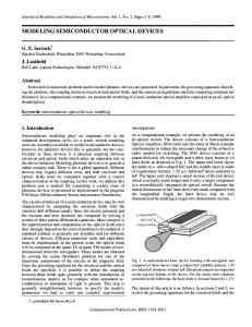
contains 226 dice and takes 10-12 weeks to process. A cross section of the device is provided in Figure 3.1.
Figure 3.1. Cross section of semiconductor device from an SRC-member company. The different layers of processing are shown.
In developing a data test bed for this and future research, four areas of evaluation were considered: 1) process data, 2) defectivity data, 3) class probe, and 4) unit probe. Process Data. As lots move through the fabrication process, many measurements are taken at different stages to gauge how the process is performing. For example, critical dimension measurements may be taken after an etching process to ensure the correct amount of material was etched. These process measurements also measure critical dimensions and overlay for the photo processes, remaining
44
oxides at etch, changes in oxide thicknesses, etch endpoint times, and more. Several process parameters are recorded at each layer of fabrication. Process data are automatically recorded in a tool, such as DataLog. Though DataLog can have data integrity issues, it is used commonly in examining process data in SPC graphs. DataLog isn’t a tool often used by the device engineer. He or she relies more on the defectivity, class probe (also referred to as parametric or electrical test), and yield data. If there is a processing concern, he or she directs questions to the process owner. Data are pulled from DataLog by using what is known as an Area – Logbook – Process or ALP. An area will usually denote the type of process and measurement. For instance, E_CD_SEM measures the critical dimensions for the etch process. The “logbook” is often a specified piece of equipment or a specified layer for the part. Often the “process” is the part name or an equipment name. Queries can be used to extract raw or summary data and can be limited by date. The process data extracted for this project are those applicable to the device of interest during the time period of April 1, 2006 through September 30, 2006. Process data are measured on two wafers from each lot after each layer of fabrication (see Figure 3.3). The data files compiled for this project include both the raw and summary data for each process parameter. This allows researchers to examine the control charts, such as the one shown in Figure 3.2 for defect density, as well as using the raw or summary data for modeling purposes. Some of the process measurements included in this data set are given in Table 3.1.
45
Xbar-R Chart of TOTALDD-RAW Sample M ean
0.45
1
0.30
1
1
U C L=0.2267 _ _ X=0.0595
0.15 0.00
LC L=-0.1076 11 4: :1
6 06 6 20 00 1/ /2 0 / 22 4 / 0 04
44 4: :5 15 0
06 20 4/ 0 5/
7
11 0: :4 6 00 /2 23 / 05
50 3: :4 21 06
06 20 6/ /0
30 3: :3 22 0
26 6/
6 00 /2
2 :4 23 2: 20 5/ /1 07
06
17
51 3: :4 6 00 /2 28 / 07
04 8: :4 14 0
06 20 3/ 2 8/
9 :0 56 9:
6 00 /2 12 / 09
23
19 8: :4 6 00 /2 26 / 09
57 5: :3 19
Sample Range
ST O P 1
2.0 1.5
1
1.0
1
1
1
1
1
1
1
U _ C L=0.693 R=0.346 LC L=0
0.5 0.0
04
06 20 1/ /0
1 :1 14 6:
06 20 2/ /2 4 0
4 :5 15
4 :4
05
4 /0
6 00 /2
1 :1 40 7:
06 20 3/ /2 5 0
50 3: :4 21
06 20 6/ /0 6 0
30 3: :3 22 6 /2 06
6 00 /2
2 :4 23 2: 20 5/ /1 07
06
51 3: :4 17
06 20 8/ /2 7 0
04 8: :4 14
6 00 /2 23 / 08
56 9:
9 :0
06 20 2/ /1 9 0
19 8: :4 23
06 20 6/ /2 9 0
57 5: :3 19
ST O P
Figure 3.2. X-bar and R chart for Defect Densities for the device studied. The raw data extracted from the process allow researchers to examine the process in many different ways, including the use of control charts to detect special cause variation. Table 3.1. Process Measurements in Dataset Process Yield Critical dimensions Etch Overlay Oxide Remaining oxide Diffusion thickness
Measurements recorded Defect counts and defect densities CD bar CD bar delta to target Etch endpoint time X offset Y offset Pre-oxide thickness Post-oxide thickness Remaining oxide Damaged silicon Thickness Top, center, and bottom wafer ranges
46
Defectivity. Defects are detected by comparative techniques using high-powered visual equipment. Defects are found by a machine comparing one die to the next and noting any differences. If there is a difference between the two die, a third dice is checked to determine which one contains the defect. These data are often used to look at significant problems with a wafer. At the SRC-member company contributing to this project, defectivity is measured using KLA machines and is recorded in a system called KLARITY. KLARITY stores both die- and wafer-level data. However, KLARITY is not directly linked to the database that contains the unit probe data for the die. A program has been written to link the two when both types of corresponding data are needed. The size of the defect is usually not of concern to the engineers. However, the visual images produced from selected defects are often key in determining the root causes for problems. Device engineers can access these images from their computers easily. Defects such as scratches can be easily seen at a high level, and SEM (Scanning Electron Microscope) images are also available. These images help the engineer quickly determine if the defect will cause a fatal flaw in the dice. Sometimes defects will cause a die to fail at unit probe (known as a fault), but other times (this is somewhat dependent on the location on the die and the critical area), the die will function properly regardless of the defect. KLA data are recorded at ten layers of this device. They are given in Table 3.2. 47
Table 3.2. Description of the Layers Involved in Defectivity Scans Layer Layer 1 Layer 2 Layer 3 Layer 4 Layer 5 Layer 6 Layer 7 Layer 8 Layer 9 Layer 10
Description Active Poly 1 Flash Flash Drain Salicide Contact Metal 1 Via 1 Metal 2 Metal 3
Defectivity measures are not performed on every wafer. For this device, they are usually conducted on every tenth lot that is fabricated. From each of these test lots, two wafers (#2 and #21) are tested (see Figure 3.3). The dataset includes the wafers that had KLA data that were tested at unit probe between June 1, 2006 and September 30, 2006. This dataset includes 136 lots. The KLA data in the dataset compiled include the lot number, wafer number, x- and y- coordinates of the die, the layer where the testing was performed, the defect number (such as the 10th defect found, etc.), the classification if the defect was classified, and the corresponding bin code from unit probe. The process data and the defectivity data are the two types of in-line test measures available in the dataset. Toward the end of the fabrication process, class probe and bin data are collected. Figure 3.3 shows the frequency of the wafer testing for the various data types and the inconsistencies present in the sampling structure across the different data types. 48
PROCESS DATA (2 wafers each lot tested at every layer, wafers 1 & 2)
CLASS PROBE (9 SITES)
BIN DATA by die
(wafers 1, 12, 25)
(pass/fail or bin counts)
DEFECTIVITY (10 LAYERS) (every 10 lots, wafers 2, 21)
End-of-line Tests
In-line Tests
1 Lot = 25 Wafers
Figure 3.3. Sampling strategies by lot for different data types. Process data are taken from wafers 1 and 2 in each lot. For lots selected for defectivity scans, wafers 2 and 21 are scanned. Class probe tests are done on wafers 1, 12, and 25 for a lot, but are conducted on 9 designated sites on the wafer. Bin data are recorded for each die after wafer probe has been completed.
Class Probe. Class probe data are recorded from electrical tests performed on the “streets” of the wafer. These tests are conducted at different reticule sites that vary from device to device. For the device studied in this research, there are 9 places where the wafers are tested for parametric data, such as L-Effective, WEffective, and threshold voltage (VT). Due to this type of test, these data are recorded at the wafer level, not the die level. These data are helpful to engineers in determining where in the process problems may have occurred that impact functionality of the device. There are over 400 parameters that are tested at class probe, but these are only done on 49
wafers 1, 12, and 25 for each lot. However, reliability tests, which include 17 or 18 parameters, are performed on 5 sites on every wafer for this device. These are stored differently in dataPOWER so device engineers as well as process engineers are able to use the information. Some parameters are closely linked to specific processes. For instance, if a problem occurs with the L-Effective, the device engineer knows the process most likely responsible for this deviation, whereas when problems occur with WEffective, which is formed in several different steps, it is harder to determine the root cause. The dataset compiled includes class probe data for all wafers tested between June 1, 2006 and September 30, 2006. In addition, the company provided a list of 109 “watchdog” parameters that are more important to refine the search from the 400+ to these. The engineer also provided a list of about 40 of these “watchdog” parameters that he considers most important.
Unit Probe. The unit probe (sometimes called wafer sort) data are needed to determine the final adequacy of the product. Testing is performed to determine if the die are good or bad. When a die fails, its failure is categorized into a specific “bin.” These various bins are coded for a variety of failure modes. These failures can be viewed on a wafer map as shown in Figure 3. 4.
50
Figure 3.4. A wafer map. Different colors of dice on the wafer map indicated different failure bin assignments based on unit probe tests. For this device, two passes of testing are required. The first pass includes all functional testing. If a wafer passes the first pass of testing, each die is classified into BIN 250, and it is baked for 72 hours before the memory is checked for retention. If a die passes this second test, it is classified as “BIN 1” and is shippable. If the wafer fails the first pass, it will be scrapped unless there are special circumstances such as the engineer hasn’t readjusted the specification limits after a change. The engineer may indicate if the wafer should be retested. Hence, sometimes there are multiple sets of bin data for the same wafer. The failure limits for specific bins are kept in a specific program where the data can be easily accessed by the engineer to examine specific failures.
51
Use of the Dataset
As described in Chapter 1, this dissertation focuses on developing modeling strategies using GLMs to predict wafer sort outcomes at unit probe testing based on defect counts on the process layers. The other components of this dataset (class probe and process data) have been useful in furthering the work of Kumar (2006) through the work of Chang (2010) at the University of Washington. These data have been used to help further advance the methodology of hGLMs described in Chapter 2. The remainder of this chapter will describe the steps taken to refine the defect count and wafer sort data from their raw forms in the dataset to a useable form for modeling purposes.
Data Refining for GLM Model Building Data Integration. For GLM models that use defectivity data for predictors, the defect metrology data and the wafer sort yield data first need to be integrated by die for die-level analyses to be performed. This can be done a number of ways, including automatic or manual methods. If using software such as DataPower, these data may already be integrated and be easy to extract together. If multiple databases are used to store the various types of data recorded during the fabrication and testing process, though, running queries in both can sometimes require advanced coding expertise, especially if the location coordinates of the dice are constructed differently for different tests, specifically, defect metrology and wafer sort.
52
Data Aggregation. Perhaps the most time-consuming task is taking the integrated data and aggregating them into a form that will be usable for model building. Table 3.3 contains an example of raw, integrated data extracted from a database. Rows showing dice with multiple defects on a layer are highlighted in bold text. While these integrated data contain the lot number, wafer number, layer number, die location (given in x- and y-coordinates), and the final bin assigned at wafer sort for each identified defect found during the scan, this arrangement of the data is not useful for common statistical packages such as Minitab or JMP that can create the desired models. For example, in Table 3.3, the die from Lot 1, Wafer 2, with coordinates (9, 1) has one defect on Layer 1 and three defects on Layer 2, so it is displayed on four different rows. The data need to be aggregated such that each die (or wafer for wafer-level modeling) is a row, and the total number of defects in each layer is given in a separate column with the column containing the wafer sort test result remaining. An example of the necessary aggregation is shown in Table 3.4. Here, the die from Lot 1, Wafer 2 with coordinates (9, 1) is summarized in a single row showing it had one defect detected in Layer 1 and three defects on Layer 2. Also, if using a binomial response (pass or fail), the failure bin data should be converted to reflect the appropriate binomial response rather than a specific bin number as shown in the far right column.
53
Table 3.3. Raw Data for Each Defect After Integration Lot ID 1 1 1 1 1 1 1 1 1 1 1 1 1 1 1 1 1 1 1 1 1 1 1 1 1
Wafer ID 2 2 2 2 2 2 2 2 2 2 2 2 2 2 2 2 2 2 2 2 2 2 2 2 2
Layer ID 1 1 1 1 1 1 1 1 1 1 1 2 2 2 2 2 2 2 2 2 2 2 2 2 2
Die Coordinate X 2 4 5 8 8 9 11 13 18 18 18 1 1 3 4 5 5 5 7 9 9 9 10 11 11
Die Coordinate Y 7 3 7 8 16 1 17 16 8 9 10 9 9 12 15 6 8 10 11 1 1 1 1 1 1
Failure Bin Number 1 1 1 24 1 7 1 1 1 7 1 1 1 1 1 1 1 42 1 7 7 7 77 1 1
Defectivity measures were taken after each of ten layers in the fabrication process. These measures include a count of the number of defects found on each layer for a particular die. Die x- and y-coordinates were used to calculate radial distance from the center and also to assign a die quadrant category. An example of the types of data used for model building is shown in Table 3.5. Additional factors, such as defect size, stepper fields, indicator variables for killer or nonkiller classified defects, and location of the defect within the die may also be included as predictors, but these data were not available in the dataset.
54
Table 3.4. Aggregated Data for Individual Dice
LotID 1 1 1 1 1 1 1 1 1 1 1 1 1 1 1 1 1 1 1 1 1 1 1 1 1
WaferID 2 2 2 2 2 2 2 2 2 2 2 2 2 2 2 2 2 2 2 2 2 2 2 2 2
DieX 1 2 3 4 4 5 5 5 5 5 5 6 7 7 7 8 8 9 10 11 11 13 18 18 18
DieY 9 7 12 3 15 6 7 8 10 11 15 15 3 11 15 8 16 1 1 1 17 16 8 9 10
Defects on Layer 1 0 1 0 1 0 0 1 0 0 1 1 1 1 0 1 1 1 1 0 0 1 1 1 1 1
Defects on Layer 2 2 0 1 0 1 1 0 1 1 0 0 0 0 1 0 0 0 3 1 2 1 1 1 1 1
Bin 1 1 1 1 1 1 1 1 42 1 1 1 1 1 1 24 1 7 77 1 1 1 1 7 1
Fail = 1 0 0 0 0 0 0 0 0 1 0 0 0 0 0 0 1 0 1 1 0 0 0 0 1 0
Table 3.5. Subset of Data for Analysis Lot Number 1 1 1 1 1 1 1 1 1 1 1 1 1 1 1 1 1
Wafer ID 2 2 2 2 2 2 2 2 2 2 2 2 2 2 2 2 2
Die X 2 2 2 2 3 4 5 5 5 5 6 6 7 7 7 7 7
Die Radial Die Layer Layer Layer Layer Layer Layer Layer Layer Layer Layer Response Y Distance Quadrant 1 2 3 4 5 6 7 8 9 10 (Fail = 1) 7 7.28 3 1 0 0 0 0 0 0 0 0 0 0 10 7.07 2 0 0 0 0 0 1 0 0 0 0 0 11 7.28 2 0 0 1 0 0 0 0 0 0 0 0 12 7.62 2 0 0 1 0 0 0 0 0 0 0 0 12 6.71 2 0 1 0 0 0 0 0 0 0 0 0 3 7.81 3 1 0 0 0 0 0 0 0 0 0 0 6 5.00 3 0 1 0 0 0 0 0 0 0 0 0 7 4.47 3 1 0 0 0 0 0 0 0 0 0 0 11 4.47 2 1 0 0 0 0 0 0 0 0 0 0 15 7.21 2 1 0 0 0 0 0 0 0 0 0 0 3 6.71 3 0 0 1 0 0 0 0 0 0 0 0 15 6.71 2 1 0 0 0 0 0 0 0 0 0 0 2 7.28 3 0 0 0 1 0 0 0 0 0 0 0 3 6.32 3 1 0 0 0 0 0 0 0 0 0 0 5 4.47 3 0 0 1 0 0 0 0 0 0 0 0 7 2.83 3 0 0 0 0 1 0 0 0 0 0 1 11 2.83 2 0 1 0 0 0 0 0 0 0 0 0
55
Managing outliers. With the large quantities of data available in the semiconductor industry, there is a question of which data, if any, should be removed for model building. While many algorithms exist to detect outliers, clear cutoffs for removing data are difficult to determine. Figure 3.4 illustrates the large number of possible outliers looking at the total number of defects per die. For the die-level training set, the median is 1.0, but the mean is 2.571 defects per die. Also, the third quartile is 2.0 and the maximum value is 218. This demonstrates the presence of unusual observations that may have a strong impact on model building. To explore the effects of removing outliers, the models built in the study described in Chapter 4 were built three times from the training dataset. The distribution for the die-level training dataset showed the 97.5th percentile to be 9 total defects on a die, and the 95th percentile was 5 total defects on a die. The dice with more than 9 and more than 5 total defects were removed from the data set using a one-sided trimmed means outlier detection approach with p=0.025 and p=0.05, respectively. Hu and Sung (2004) show trimmed means to be an appropriate method for outlier detection that has higher efficiency than using median. This method unifies mean and median in a dataset. While their study uses two-sided trimmed means with p=0.15, this more conservative approach will allow the most common occurrences of defect distributions on layers to be examined while constructing useful models. No points were removed from the test dataset that was used for validation purposes described in Chapters 4, 5, and 6. 56
Summary for Total Defects per die (Die Level Training Set) A nderson-D arling N ormality Test
0
30
60
90
120
150
180
210
A -S quared P -V alue