the colored stripes allow recovering absolute depths at coarse resolution ... using commercial off the shelf hardware, which distorts ...... 1st Int. Symp. on 3D Data.
Sensing Deforming and Moving Objects with Commercial Off the Shelf Hardware Philip Fong Florian Buron Department of Computer Science Stanford University, Stanford, California, USA {fongpwf, fburon}@robotics.stanford.edu Abstract In many application areas, there exists a crucial need for capturing 3D videos of fast moving and/or deforming objects. A 3D video is a sequence of 3D representations at high time and space resolution. Although many 3D sensing techniques are available, most cannot deal with dynamic scenes (e.g. laser scanning), can only deal with textured surfaces (e.g. stereo vision) and/or require expensive specialized hardware. This paper presents a technique to compute high-resolution range maps from single images of moving and deformable objects. A camera observes the deformation of a projected light pattern that combines a set of parallel colored stripes and a perpendicular set of sinusoidal intensity stripes. While the colored stripes allow recovering absolute depths at coarse resolution, the sinusoidal intensity stripes give dense relative depths. This twofold pattern makes it possible to extract a high-resolution range map from each image captured by the camera. This approach is based on sound mathematical principles, but its implementation requires giving great care to a number of low-level details. In particular, the sensor has been implemented using commercial off the shelf hardware, which distorts sensed and transmitted signals in many ways. A novel method was developed to characterize and compensate for distortions due to chromatic aberrations. The sensor has been tested on several moving and deforming objects.
1. Introduction Considerable research has gone into developing techniques to sense the 3D geometry of objects. However, such techniques have focused on rigid objects and quasi-static scenes. In many applications, there is a need for sensing fast moving and/or deforming objects. For example, capturing the deformation of real objects could be used in surgical simulation to model human tissues and organs. Modeling fabric and rope deformation is of great interest for the video games and film industries. Another application is vehicle crash tests where analysis of the deforming geometry is of direct importance. Real-time sensing of moving and deforming objects can also be used for feedback in robotic manipulation and navigation.
These applications require a high-resolution range sensing technique that makes minimal assumptions about the type of objects sensed and the types of motions occurring in the scene. This paper describes a range sensing technique that extracts depth information in the entire field of view from single images and is suitable for untextured objects. We also discuss and address some of the challenges of implementing this system on commercial of the shelf (COTS) hardware. COTS hardware is not designed specifically for this task and distortions acceptable to the hardware’s target application can lead to performance degradation in a range sensor. In particular, we focus on characterizing and compensating for color dependant distortions such as chromatic aberration in lenses.
2. Related Work Previous research in range sensing can be divided into time of flight techniques and triangulation techniques. Among time of flight systems, radar and lidar systems generally provide sparse depth maps. Shaped light pulse systems [1] can produce dense range maps at relatively fast frame rates but have low depth resolution and require expensive specialized hardware. Triangulation based systems include laser stripe scanning, stereovision, and pattern-based structured light methods. In these approaches, corresponding features in different viewpoints are found and their 3D positions are computed by intersecting rays from each viewpoint. These methods are distinguished by how they solve the correspondence problem. Laser scanners project a single plane of light and scan across the scene. This limits their application to rigid static objects. Stereovision, which finds correspondences by matching pairs of features from two images, often fails on objects with no texture or repeating textures. It has been successfully applied to moving and deforming textured cloth [2]. Pattern-based structured light techniques are capable of producing a dense range map of an entire scene by projecting a pattern and observing how it is changed from another viewpoint. Here finding correspondences is reduced to finding spatially and/or temporally unique features encoded into the pattern. In methods that only rely on single images, range maps can be produced at the
Camera/World Frame ZW XW
YCI
px
Target Object(s)
XCI YW
py
ZP
pz
XP
XPI
YPI
YP Projector Frame
Fig. 1 Projected pattern
Fig. 2 System geometry
video frame rate (in real-time or postprocessed). Multiimage techniques typically give higher quality range maps, but rely on temporal coherence limiting the speed of motions in the scene and often produce range maps at a rate lower than the video frame rate. Pattern-based techniques differ in the way the information is encoded in the pattern. Intensity ramp patterns [3] are sensitive to noise and reflectance variations. Techniques using Moiré gratings and sinusoids [4,5,6] are much more resistant to noise and reflectance variations, but requires both knowledge of the topology and points of known depth in the scene. In systems using black and white stripes [7,8] or colored stripes [9,10,11] the resolution of the range map obtained from a single image is limited by the discrete number of possible pattern encodings. Higher resolution is attained by using a temporal sequence of images and patterns. This limits their use to rigid or slowly moving objects. In contrast, the technique presented here scales with camera resolution even while using single images. Spacetime stereo [12] is a method that performs stereo matching over space and time windows on scenes illuminated by arbitrarily varying patterns. In [8], a series of vertical stripes are used with a few diagonal stripes to disambiguate them. The technique presented here also uses a pattern with repeating features combined with additional unique features.
more robust because the color and sinusoidal components provide complementary information. The colored stripe boundaries give sparse, but absolute depths, while the sinusoid gives dense relative depths. These points are used as known points in the sinusoid processing. The sinusoidal component is resistant to reflectance variations in the scene and only a few correctly sensed color transitions (also called color edges) are needed as start points. A sinusoidal pattern also avoids the need to do any sub-pixel location estimation of pattern features (e.g. transitions). The depths are computed at pixel locations. Also, since dense ranges are computed from a pattern with no sharp edges, the focus depth of field of the projector or camera does not limit the sensor’s working volume. A pattern of vertical colored stripes with a horizontal sinusoid overlaid (see Fig. 1) is projected on to the scene by a standard LCD projector and images are captured from a different viewpoint with a color camera. The sinusoid of intensity is embedded in the value channel and the colored stripes are embedded in the hue channel in HSV color space. Orienting the color transitions perpendicular to the intensity variation makes them easier to find and allows the sinusoid frequency to be independent of the color stripe frequency. Each frame can be processed independently to recover depth information. Pixels are given color labels and scores by a Bayesian classifier. The stripe transitions are identified, labeled, and scored according to the color labels of pixels adjacent to each boundary. The scene is segmented into regions using a snake technique [13] and the luminance component in each region is processed to recover the dense depth map using the color transition depths as starting points. Processing each frame independently eliminates the need for temporal coherence. The scene can change significantly between frames without affecting the depth recovery. However, temporal coherence may still be used to improve performance.
3. Overview 3.1. Basic Operation The technique described here combines features of color stripe and sinusoidal triangulation systems. We use color stripes to get sparse but absolute depth values and a sinusoid to propagate these values and get a highresolution range map. To guide the propagation we segment the image into regions that do not contain any depth discontinuities. Compared to patterns used in previous work, which employ either color or luminance alone, this pattern is
3.2. System Geometry Fig. 2 shows the geometric configuration and coordinate frames of the camera and projector. The world coordinate frame, W, coincides with the camera coordinate frame which is centered at the camera lens optical center with XW pointing to the right, YW pointing down, and ZW pointing out of the camera lens along the optical axis. The projector frame, P, is centered at the projector lens optical center which is located at W(px, py, pz) and the axes are aligned with those of the world frame. In practice, the optical axis of the projector and camera may not be parallel but rectifying the projected pattern makes a parallel virtual axis. It is often useful for them to be verging together at a point near the object of interest. Points in the world are mapped onto the projector and camera normalized virtual image planes (located at z=1) using a pinhole lens model: W W x y CI x = W , CIy = W z z (1) P P x PI y PI x= P , y= P z z Note that CI(x,y) = W(x,y,1) and PI(x,y) = P(x,y,1). The mapping from real image plane coordinates to the normalized virtual coordinates is done with a projection model that accounts for lens distortion [14] and by warping the projected pattern and captured images. Computing the range map is then the same as computing the z value for each pixel on the image plane of the camera.
4. Computing Depth 4.1. Depth from Colored Stripes The absolute depths of points in the scene can be found by detecting the color stripe transitions in the acquired image and triangulating with the locations of the stripe transitions in the projected pattern. The color part of the projected pattern consists of a set of colors, C={c0, …, cn} arranged into a sequence (b0, …, bm) bi ∈ C of vertical stripes such that: 1. bj≠bj+1, i.e. consecutive colors are different. 2. bj≠bk or bj+1≠bk+1 for j≠k, i.e. each transition appears once. Using more colors leads to a greater number of possible transitions, but the colors are more difficult to distinguish. In our case, since the sinusoid is used to get the dense range map, having a large number of transitions is not critical. In most of the results presented in this paper, six colors were used allowing 30 unique transitions. In the projected pattern, each color transition uniquely identifies a vertical plane. On each scanline (constant CIy), if a transition is found at CIx and
corresponds to the transition located at PIx in the projected pattern, the z value of the point in the scene corresponding to the pixel CI(x,y) is: W
z ( CI x,CI y ) =
W
pX − PI x W pZ . CI x − PI x
(2)
4.2. Recovering the Color Transitions In captured images, a Bayesian classifier determines the colors of the pixels. The probability distributions are estimated by fitting gaussians to training images of the scene with a projected “pattern” of only one color. The images are converted to HSV space giving hues h(x,y), saturations s(x,y), and values v(x,y). For each color, c, the mean, µc, and variance σc of the hues are computed and stored. Colors in the pattern should be chosen so that the overlap in the gaussians is minimized. Our technique is robust to incorrectly classified pixels because all transitions detected in a region are aggregated to form a guess for the phase unwrapping (see section 4.5). A captured image the hue channel is processed one horizontal line at a time. There are several techniques to locate color edges, such as the consistency measure used in [9]. A simpler method is to look at the difference in hue between consecutive pixels. For each group of pixels whose absolute hue difference (taking into account the circular nature of hue) exceeds a set threshold, pick the pixel with the maximum difference to be the location of a transition. Once an edge is found, it is labeled with a transition and given a score based on the color scores of windows of pixels on each side of the transition. If the color scores are not consistent with a projected transition (e.g. both sides are the same color), the transition is ignored. The scores reflect how confident we are of the label of the transition.
4.3 Depth from Sinusoids The depth at each pixel is computed from the apparent phase shift between the projected and observed sinusoids. On the projector image plane, the luminance of the projected pattern is: v( PI x, PI y ) = A cos(ωPI y ) + C (3) where ω is the frequency. A and C are chosen to maximize the use of the projector’s dynamic range and ω is set smaller than the camera’s and projector’s Nyquist frequencies. Converting to world coordinates and projecting into the world yields: W y−W p (4) v( W x, W y, W z ) = A cos ω W W Y + C . z − pZ The camera sees on its image plane:
v(CIx,CI y) = R( W x, W y, W z (CIx,CI y)) × W z(CIx,CI y)CIy − W p cos ω W CI CI W Y + N ( W x, W y, W z (CIx,CI y)) z ( x, y)− pZ (5) where R(x,y,z) is due to the reflectance of the surface at (x,y,z) and N(x,y,z) is due to noise and ambient light. Computing the depth map is recovering Wz(CIx,CIy). Eq. (5) gives: v( CI x, CI y ) = A cos ωCI y − θ( CI x, CI y ) , (6)
(
)
− p y + pY . θ( CI x, CI y ) = ω W CIZ CI (7) W z ( x, y ) − p Z In this formulation, θ can be seen as modulating the phase or frequency of the original sinusoid. We will refer to it as the phase. θ w = arctan 2(sin(θ), cos(θ)) , the W
CI
W
wrapped version of θ, can be recovered by multiplying v(CIx,CIy) by cos(ωCIy) and low-pass filtering (digital demodulation) [5,6]. θ is recovered from θw by phase unwrapping as described in section 4.5. Given θ(CIx,CIy), Wz(CIx,CIy) is given by:
ω(− W pZ CI y + W pY ) W + pZ (8) θ(CIx,CI y) The 3D locations of the points are found by projecting back into the world coordinate frame. W
z (CIx,CI y) =
4.4. Segmentation Using Snakes and Phase Unwrapping The depth cannot be computed from the θw found with the sinusoid pattern processing because we need θ = θw + k2π to compute the depth and the integer k cannot be recovered from the sinusoid. This ambiguity is due to the periodic nature of a sinusoid. However, if the phase (or the depth) of one pixel is known (for example using the color stripes), we can assume that the adjacent pixels do not differ than more than 2π and compute the θ value of the adjacent pixels accordingly. Performing this propagation is called phase unwrapping [15]. To perform phase unwrapping, we need to segment our image in regions such that in each region the difference in θ between two adjacent pixels is always less than 2π. There exist various techniques to segment images. We chose the snake (or active contour) technique [13]. A snake is a closed contour, which is deforming to fit the borders of the region we want to segment. Each point of the snake is moved iteratively based on the various forces applied to it until it reaches an equilibrium. This technique is known to give good results for many problems and has the advantage of being able to bridge across small gaps in the boundary of a region we want to segment. This property is very important in our case.
We decided to base the segmentation on the phase variance (defined in [15]) of the image. The phase variance is a measure of how fast the phase of a pixel changes compared to its neighbors. A large change in phase corresponds to a discontinuity in depth and is interpreted as boundaries in our image. Phase variance has been effectively employed in phase unwrapping for applications such as synthetic aperture radar and magnetic resonance imaging [15]. The segmentation is initialized as a small circle centered randomly in the yet unsegmented region of the phase variance image such that it covers a uniform area of small phase variance values. Then, each snake point moves under the influence of three forces applied to it until equilibrium is reached: − An expansion force: Contrary to most snakes in the literature, our snake is expanding. Each snake point P is subject to a constant force pointing toward the outside of the region encircled by the snake and orthogonal to the tangent at P. − An image force: The snake expansion is locally stopped when it reaches regions of high phase variance. − A rigidity force: Each snake point is subject to a force that resists high contour curvatures. This prevents the snake from flooding into other regions through the small gaps. Regions that do not contain any detected color edges are merged with neighboring regions. Since this segmentation is based only on phase variance, it could fail if there is a long depth discontinuity that corresponds to a phase difference of a multiple of 2π. But this is very unlikely to happen because the depth difference corresponding to a phase difference of 2π varies with position. We have never encountered this problem in our experiments.
4.5. Phase Unwrapping Before unwrapping begins, guesses for θ are computed from the detected color edges by applying (2) and (7) to each edge. The score of each guess is the score, ES, of the edge. The unwrapping of each region starts at the center of the initial circle of the snake. Then the pixel with the lowest phase variance among pixels that border unwrapped pixels is unwrapped. This proceeds until the entire region is unwrapped in a way similar to the quality map algorithm in [15]. Once a region is unwrapped, the offset for the region needs to be computed from the guesses encountered in the region. We have θu, which is offset from θ by an integral multiple of 2π. θ( x, y ) = θ u ( x, y ) + 2πk (9)
k is computed by rounding to the nearest integer the guess score weighted median of the difference between encountered guesses and θu divided by 2π. Using the weighted median provides robustness against bad guesses from misclassified colors or falsely detected edges. In our experiments, incorrect offsets are only used in regions containing a small number of guesses.
5. Calibration Calibrating a projector-camera system is more difficult than calibrating a dual camera system. Standard camera calibration techniques are based on finding the location in the image plane of known 3D points in the world space [14]. To calibrate a projector, a camera needs to be used to observe a projected pattern. The known points are on the projector image plane and the corresponding points are found in the world using the camera. This often leads to many more sources of error in the calibration. In this work, the 3D world coordinates were found by calibrating the camera first and using the camera to locate the points of a projected checkerboard pattern overlaid on a printed planar checkerboard pattern. This provides a basic set of parameters describing the camera and projector. Use of color presents a special challenge in using COTS projectors and cameras. Color misalignment caused noticeable artifacts in our range maps. The colored stripe processing is robust to some color misalignment because the results are only used as guesses for the phase unwrapping and only need to be within 2π of the correct result. If the misalignment causes the sinusoidal pattern to be shifted, it will result in a systematic error in the depth. This is especially evident when the shift between colored stripes causes ridges to appear in the range map. Fig 3 shows the reconstruction of a surface at about 1000 mm from the sensor. The artifacts are clearly visible. Several sources contributed to the color misalignment. Both the projector and camera lenses exhibit chromatic aberration. The typical C-mount lens such as the one used in our experiments is designed for
Fig. 3 3D reconstruction of a surface sensed from about 1 m away.
monochrome closed circuit TV (security camera) or industrial machine vision applications where chromatic aberration is irrelevant. LCD projectors are normally used to show presentations where audience members don’t notice small amounts of chromatic distortion. It is not used as a scientific instrument. Specialized lenses that compensate for chromatic aberration could have been used in the camera but would be much more expensive. The projector lens is not designed to be replaceable. Additional color distortion in the projector is due to color being produced by three separate LCD panels, which could be misaligned, and their associated optical paths may not be perfectly matched. Chromatic distortion can be divided into traverse (lateral) and longitudinal components. Longitudinal distortion results in the colors not being in focus in the same plane and cannot be easily compensated for after the image has been captured. The sensor is not very sensitive to this effect because the sinusoid has no sharp edges. Lateral chromatic aberration can be modeled by focal length and distortion parameters that vary with wavelength. Stretching the different color channels of the captured image appropriately can compensate for it. In many cameras (including ours), color is sensed by a Bayer pattern sensor, which reduces the effective resolution. This makes it difficult to find the focal length and distortion parameters for each color channel directly. Additionally, the projector can only be calibrated through images captured through the camera lens, which will show the combined distortions of both the projector and camera. In our system we chose the green image channel as the reference. Green has a refraction index between red and blue and the camera has the highest effective resolution in green due to the Bayer pattern filter and is most sensitive to green. Differences observed in the red (blue) channels relative to green are modeled with three parameters: α the ratio of the green camera focal length to the red (blue) camera focal length, β the ratio of the green projector focal length to the red (blue) projector focal length and γ the shift in direction of the Y axis of the red (blue) channel relative to the green channel in the projector. A shift does not need to be considered in the camera because color is sensed through a Bayer pattern filter in the camera and the color channels cannot be misaligned in the camera. We only consider a shift in the Y axis direction because shifts in the X direction do not affect the projected sinusoid. Shifts in X do affect the color transitions but as previously discussed they do not need to be accurately located. If these parameters are known we can compensate for the distortion. The projected sinusoid (3) is modified for each color channel by: v( PI x, PI y ) = A cos(ω(β PI y + γ )) + C . (10)
For the camera, the acquired images’ red (blue) channel is scaled by α and resampled. α, β, and γ can be estimated from the measured phases θg computed from the green channel and θr (θb) computed from the red (blue) channel of a white sinusoid. In the compensated images each channel should have the same phase at every point. We minimize: (11) ∑ (θ s ( xα, yα) − θ g ( x, y )) 2 Q
where Q is a set of points in camera images and θs simulates the effect of compensating for the shift and focal length differences and is computed from θr (θb) by: θs ( x, y ) = β(θ r ( x, y ) − ω(( α1 − 1) y − γ ) . (12) The
ω(( α1
− 1) y term accounts for the effective change in
sampling period in demodulation due to the change in camera focal length. In our experiments, the optimization was done over measurements made of surfaces about 540 mm, 690 mm, 825 mm, and 1075 mm from the sensor using a pattern of a white sinusoid. The effectiveness of compensation was evaluated by taking range maps of a set of four surfaces sensed at about 500 mm, 700 mm, 1000 mm, and 1200 mm from the sensor. Each surface was imaged using a white sinusoid for reference and the multi-colored sinusoid with and without compensation for comparison. For each range map we defined the error by the difference between the depths computed from the green channel of the white sinusoid to the depths computed from the colored stripe image. Fig. 4 shows a cross-section of the error on a surface at about 1000 mm. This cross-section is along the red line in fig. 3 and 5 where the combined effects of the camera and projector are the greatest. Fig. 5 shows the reconstruction of the surface sensed using compensation. Applying correction reduces the artifacts significantly. Over the whole data set, the compensated RMS error is on Error from Green Reference
3 2
Error (mm)
1
Fig. 5 3D reconstruction of a surface sensed from about 1m away using compensation.
average 36% of the uncorrected RMS error. The compensated RMS error is 0.05% of the average measured distance to each surface. For instance, on the surface at about 1000 mm, the RMS error is 0.48 mm. The remaining errors are likely due to variation in the higher order lens distortion between colors in the camera and projector and the unmodeled effects of the projector’s optics (such as rotation of the LCDs relative to each other). These results were obtained by optimizing α, β, and γ over a fairly large working volume (over 700 mm). It is likely that the error would be further reduced if only a small working volume was desired.
6. Experimental Results The results shown here were obtained with a Viewsonic PJ551 LCD projector at a resolution of 1024x768. Images were captured using a Basler A602fc camera at 640x480.
6.1. Toy Duck We captured a range map of a plastic toy duck. It was about 47 cm from the sensor. For reference a Cyberware 3030MS laser scanner was used to scan it. The laser scan had to be manually edited to remove spurious points produced by the specularity of the plastic. Fig 6 shows a photograph, the captured image, and 3D reconstruction of the toy. Fig 7 shows a cross-section taken along the red line in Fig 6. The range map from our sensor captures the general shape but has some small
0 -1 -2 -3 -4 -5
Uncompensated Compensated -0.2
-0.1
0
0.1 x
CI
0.2
0.3
0.4
0.5
Fig. 4 Error in depth from green reference of a surface sensed with compensated and uncompensated patterns.
Fig. 6 Plastic toy duck. Photograph (left), Captured Image (mid), 3D Reconstruction (right)
Duck Cross-section
-1005
z (mm)
-1010
-1015
-1020
-1025 Cyberware 3030MS Our Sensor -1030
0
50
100
150
200
y (mm)
Fig. 7 Cross-section of toy duck corresponding to red line in Fig 6.
distortions where specular highlights were in the captured image. When aligned with the reference range map the RMS error over the parts present in both is about 0.48 mm or 0.1% of the average distance to the object.
6.2. Person Moving a Popcorn Tin We captured a sequence at 60 fps showing a person moving a popcorn tin around. The texture on the popcorn tin affects the range map by adding some small distortions and, in very dark areas, holes. However, the sensor correctly senses the person and the overall shape of the popcorn tin. In particular, the sensor does well in sensing the shirt worn by the person.
6.3. Bouncing Water Balloon A water-filled balloon was dropped onto a surface and captured at 100 fps. The sequence shows the balloon deforming as it hits the surface and bounces several times. Fig. 9 shows frames selected from the sequence. Frame 25 shows the balloon just before hitting the surface when it is still spherical. The following frames show the balloon deforming as it hits the surface and bounces up.
6.4. Discussion The range maps obtained from our sensor are quite good for a single frame technique, showing the effectiveness of a combination of a discrete color pattern and continuous sinusoidal intensity pattern. Objects were successfully sensed at wide range of distances without adjusting the sensor setup (lens focus, baseline, etc.). It works on objects moving much faster than what has been shown with multi-frame techniques. Using a static pattern allows the range map frame rate to exactly match the camera frame rate. Systems using pattern sequences are limited by the speed of both the projector and camera. Cameras faster than 500 fps are commercially available, while almost all projectors work
Fig. 8 Person with popcorn tin. Photograph of tin (top left), Captured image (top right), 3D reconstructions (bot)
at 60 fps or less. Additionally, in cases where adapting the projected pattern to the scene is unnecessary, the LCD projector can be eliminated saving cost and weight. However, the current implementation has a few drawbacks. The unwrapping process requires at least one correct phase guess in each region. The colored stripe process often produces many more than needed. But in objects that have strongly saturated colors there will be fewer guesses making the system more sensitive to segmenting errors. For example, the sensor will have difficulties on a bright red object. This can be mitigated by choosing the right set of colors in the pattern in some cases. However, if the scene contains many saturated colors it then could be very difficult to find a good set of pattern colors. Finally, this system is subject to a limitation common to all structured light approaches: the projected pattern must be brighter than the ambient light.
7. Conclusion The proposed system produces good quality dense range maps of scenes composed of moving and deforming objects at camera frame rates by using a pattern that combines color and luminance information. It makes no temporal coherence assumption and a reduced spatial coherence assumption. The spatial resolution scales with camera resolution and the temporal resolution depends on camera speed and not on projector speed.
Fig. 9 Frames 25, 28, 31, 34 and 37 of the water balloon sequence. [6] G. Sansoni, L. Biancardi, F. Docchio, and U. Minoni. “Comparative Analysis of Low-Pass Filters for the Demodulation of Projected Gratings in 3-D Adaptive Profilometry,” IEEE Tr. Instrumentation and Measurement, 43:50-55, 1994. [7] G. Sansoni, M. Carocci, and R. Rodella. “Calibration and performance evaluation of a 3-D imaging sensor based on the projection of structured light,” IEEE Tr. Instrumentation and Measurement, 49(3):628-636, 2000. [8] T. P.Koninckx, A. Griesser, and L. Van Gool. “Real-time Range Scanning of Deformable Surfaces by Adaptively Coded Structured Light,” Fourth Int. Conf. on 3-D Digital Imaging and Modeling - 3DIM03, 293-300, October 6-10, Acknowledgments 2003. [9] L. Zhang, B. Curless, and S. M. Seitz. “Rapid Shape This work is supported in part by NIH grant R33 Acquisition Using Color Structured Light and Multi-pass LM07295 and NSF grant ACI-0205671. We would like Dynamic Programming. Proc. 1st Int. Symp. on 3D Data to thank Jean-Claude Latombe for his support, assistance, Processing, Visualization, and Transmission,” Padova, and suggestions, James Davis for his invaluable help, Ken Italy, June 19-21, 2002, 24-36. Salisbury for his support and inspiring some potential [10] D. Caspi, N. Kiryati, and J. Shamir. “Range Imaging with applications, Justin Durack for implementing the Adaptive Color Structured Light. IEEE Trans. Pattern Bayesian classifier, and Keenan Wyrobeck for his Analysis and Intelligence,” 20:470-480, 1998. assistance in constructing the experimental system. [11] W. Liu, Z. Wang, G. Mu, and Z. Fang. “A Novel Profilometry with Color-coded Project Grating and its References Application in 3d Reconstruction,” 5th Asia-Pacific Conf. [1] H. Gonzales-Banos and J. Davis. “Computing depth under Communications and 4th Optoelectronics and ambient illumination using multi-shuttered light,” Proc. Communications Conf., 2:1039-1042, 1999 IEEE Comp. Soc. Conf. on Computer Vision and Pattern [12] J. Davis, R. Ramamoothi, and S. Rusinkiewicz. “Spacetime Recognition (CVPR) 2004, 2:234-241, 2004. Stereo: A Unifying Framework for Depth from [2] D. Pritchard and W. Heidrich. “Cloth Motion Capture,” Triangulation,” IEEE Conf. on Computer Vision and Computer Graphics Forum (Eurographics 2003), Pattern Recognition, 2003. 22(3):263-271, September 2003. [13] M. Kass, A. Witkin, and D. Terzopoulos. “Snakes, Active [3] B. Carrihill and R. Hummel. “Experiments with the Contour Models,” Int. J. Computer Vision, 1:321-331, intensity ratio depth sensor,” Computer Vision, Graphics, 1988. and Image Processing, 32:337-358, 1985. [14] J.Y. Bouguet. Camera Calibration Toolbox for Matlab. [4] M. Takeda and M. Kitoh. “Fourier transform profilometry http://www.vision.caltech.edu/bouguetj/calib_doc/index.ht for the automatic measurement of 3-D object shape,” ml, 2004. Applied Optics, 22:3977-3982, 1983. [15] D. Ghiglia, and M. D. Pritt. Two-dimensional Phase [5] S. Tang and Y. Y. Hung. “Fast Profilometer for the Unwrapping: Theory, Algorithms, and Software. New Automatic Measurement of 3-D Object Shapes,” Applied York: Wiley, 1998. Optics, 29:3012-3018, 1990.
The proposed technique to characterize and compensate for color distortions is effective and allows commercial off the shelf hardware to be used. At this stage, the sensor can still be improved, but works well enough to begin exploring some application areas. We are investigating how to extract from a sequence of range maps a moving and deforming dynamic mesh. This is potentially more efficient and useful than a series of range maps. For some applications a real time implementation is needed. This technique has no intrinsic properties precluding a real time implementation.