Sensitivity study using machine learning algorithms on simulated r

Sensitivity study using machine learning algorithms on simulated r-mode gravitational wave signals from newborn neutron stars Antonis Mytidis,1 Athanasios A. Panagopoulos,2 Orestis P. Panagopoulos,3 and Bernard Whiting1

arXiv:1508.02064v1 [astro-ph.IM] 9 Aug 2015

1

Department of Physics, University of Florida, 2001 Museum Road, Gainesville, FL 32611-8440, USA 2 Department of Electronics and Computer Science, University of Southampton, Southampton, UK 3 Department of Industrial Engineering and Management Systems, University of Central Florida, 12800 Pegasus Dr., Orlando, FL 32816, USA

This is a follow-up sensitivity study on r-mode gravitational wave signals from newborn neutron stars illustrating the applicability of machine learning algorithms for the detection of long-lived gravitational-wave transients. In this sensitivity study we examine three machine learning algorithms (MLAs): artificial neural networks (ANNs), support vector machines (SVMs) and constrained subspace classifiers (CSCs). The objective of this study is to compare the detection efficiency that MLAs can achieve with the efficiency of conventional detection algorithms discussed in an earlier paper. Comparisons are made using 2 distinct r-mode waveforms. For the training of the MLAs we assumed that some information about the distance to the source is given so that the training was performed over distance ranges not wider than half an order of magnitude. The results of this study suggest that machine learning algorithms are suitable for the detection of long-lived gravitational-wave transients and that when assuming knowledge of the distance to the source, MLAs are at least as efficient as conventional methods.

I.

INTRODUCTION

It was demonstrated (1998) that neutron star r-mode oscillations of any harmonic, frequency and amplitude belong to the group of non-axisymmetric modes that can be driven unstable due to gravitational radiation [3, 7, 10]. This theory suggested that (assuming the r-mode oscillation amplitude grows sufficiently large) r-mode gravitational radiation (primarily in the m = 2 harmonic) could carry away most of the angular momentum of a rapidly rotating newborn neutron star in the form of r-mode gravitational radiation. In a previous paper [9] we presented a sensitivity study of a seedless clustering detection algorithm based on r-mode waveforms predicted by the Owen et. al. 1998 model f (t) =

1
1 fo−6 + µt 6

µ = 1.1 × 10−20 |α|2

s−1 Hz6

(1)

(2)

and the gravitational radiation power given by E˙ ≈ 3.5 × 1019 f 8 |α|2 W.

(3)

This model depends on two parameters: the (dimensionless) saturation amplitude, α, of the r-mode oscillations and the initial gravitational wave spindown frequency fo . The theoretical predictions for the values of these parameters were discussed extensively in our previous paper. The values we considered for α lie in the range of 10−3 − 10−1 while the values we considered for fo lie in the interval of 600 − 1600 Hz. Due to the wide range within which the values of these parameters lie, we cannot effectively use a matched filtering algorithm. Instead, we have to develop techniques that could detect all possible distinct waveforms.

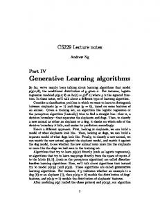
In our previous paper, a seedless clustering algorithm was used. This algorithm is based on the statistical significance of signal to noise ratios (snr) of clusters of above the threshold snr pixels. This method is not dependent on any knowledge of the signal and it can be applied generically to any longlived gravitational-wave transients. In particular, it is unable to discriminate between r-modes and other possible gravitational wave sources. Knowledge of the r-mode signal can be used to make minor modifications in the clustering algorithm, however, there was not much hope for a dramatic improvement in the efficiency. Nevertheless, we were able to recover signals of magnitude 5 times weaker than the noise. In the sensitivity study performed for the clustering algorithm, we used 9 distinct waveforms. These were chosen by taking (α, fo ) pairs using 3 values (10−1 , 10−2 , 10−3 ) for α and 3 values (700 Hz, 1100 Hz, 1500 Hz) for fo . In this sensitivity study for the MLAs, for comparison purposes, we used 2 of these waveforms: (fo = 1500 Hz, α = 0.1) and (fo = 1100 Hz, α = 0.01). These waveforms as well as their corresponding power decays are shown in Fig.1 and Fig.2 respectively. MLAs are well suited especially for cases where the signal is not precisely (but only crudely) known. This paper is based on three specific MLAs: ANN [5], SVM [4] and CSC [8]. All three methods are considered novel applications in the area of long transient gravitational wave searches. This paper is designed as follows: The next section describes the preparation of the data used for the training of the MLAs. The discussion extends to the resolution reduction of the data maps and also to the training efficiencies as a function of resolution reduction for all three MLAs. In section 3 we present a brief introduction into ANN methods, in section 4 we do the same for SVM methods and in section 5 we present a similar introduction for CSCs. In section 6 we present and discuss our results and compare the MLA efficiencies to the conventional (clustering) algorithms efficiencies. Finally, in section 7, we summarize our conclusions including topics for future work.

2 II.

Waveforms with fo = 1500Hz, α = 10−1 and fo = 1100Hz, α = 0.01

DATA PREPARATION

1600

A.

1500

1400

From equations (1) and (2) we have the two model parameters α and fo that determine the shape of the waveform. Apart from the shape, the injections that were produced for the training of the MLAs were also dependent on the pixel brightness or pixel signal-to-noise ratio (SNR). For a single pixel in the frequency-time maps (ft-maps) the SNR satisfies [11] h i ˆ ∝ Re Q ˆ ij (t, f, Ω)C ˆ ij (t, f ) SNR(t, f, Ω) (4)

1300

frequency (Hz)

Choice of the fo and α parameter values

1200

1100

1000

900

800

700 0

500

1000

1500

2000

2500

time (s)

FIG. 1. The (fo = 1500 Hz, α = 0.1) waveform is the most powerful waveform considered in our sensitivity studies both for the clustering and the MLAs. The second waveform we chose has an amplitude 25 times smaller than the first one. This waveform has parameters (fo = 1100 Hz, α = 0.01) and is approximately monochromatic for the durations our sensitivity studies were designed for. The clustering algorithm could detect the weaker signal at distances not further than a few Kpcs.

h ≈ 1.5 × 10−23



1Mpc d



f 1kHz

3 |α|.

(5)

For the construction of the injection maps we chose the 3 parameter values fo , α and h2 to be uniformly distributed within the corresponding predetermined ranges. The values of the distance d are constrained accordingly such that the above conditions are satisfied. Each injection set that was produced and used for the MLA training was limited to 11350 injection maps and 11350 noise maps. This was due to the finite amount of data that was produced during the S5 LIGO run, the computational resources available as well as the time needed to produce the 22700 maps. For each injection the waveform was randomly chosen in such a way that the α value was randomly chosen from a uniform distribution of 11350 α values in the range of 10−3 − 10−1 , the fo value was randomly chosen from a uniform distribution of 11350 fo values in the range of 600 − 1600 Hz, and for the h2 values we picked 3 ranges (for 3 separate MLA trainings), whose choice is discussed in the next paragraph.

Gravitational radiation power decay during spindown 44

10

43

10

42

power (W)

where i = 1 and j = 2 are indices corresponding to the two ˆ ij (t, f, Ω) ˆ is a filadvanced LIGO (aLIGO) detectors [1], Q ˆ [2] and ter function that depends on the source direction, Ω, ˜ ∗ (t, f )h ˜ j (t, f ) is the cross spectral density, h ˜ being Cij ≡ 2h i the Fourier transform of the gravitational wave strain amplitude h. The latter is expressed in [6] as a function of the distance d to the source, the gravitational-wave frequency f and the r-mode oscillation amplitude α, by

10

41

10

40

10

39

10

0

500

1000

1500

2000

2500

time (s)

B.

FIG. 2. These power evolutions correspond to the signals in Fig.1. We see that the blue plot corresponds to a rapidly decaying signal: within 2500 s the radiation power drops to 17% of its original value. The red plot corresponds to a power decay that dropped to only 99.9% of the initial. The power of this (red) signal is about 3 orders of magnitude lower than that of the signal plotted in blue. We chose this weak signal so that we can examine how the MLAs compare to the clustering algorithm both for powerful and weak signals.

Choice of the h2 parameter values

The results of the sensitivity study for the clustering algorithm showed that for a signal of f = 1500 Hz and α = 0.1 the detection distance was up to 1.2 Mpc. Using equation (5) we see that the conventional algorithms can detect gravitational wave strains of value h ≈ 4 × 10−24 . Values of the same order are obtained if we substitute the results for the other 8 waveforms. For example from table 1 in [9] we see that for f = 700 Hz and α = 0.01 we get a detection distance of 0.043 Mpc. Substituting in equation (5) we get h = 1.2 × 10−24 . Therefore, the value of h ≈ 10−24 will

3 become a reference point because this is the value of gravitational wave strain the MLAs will have to detect if they are shown to be at least as efficient as the conventional clustering algorithms [12]. If we consider supernova events at distances in the range from 1 Kpc to 1 Mpc then the corresponding range for the gravitational wave strain values is h ≈ 10−24 to 10−21 . Therefore, there are several approaches in determining the range of h2 values for the injection maps produced for the training of the MLAs: (i) produce one set of data with injections at distances distributed in such a way that the h2 values are uniformly distributed in the range from 10−48 to 10−42 (i.e. 10−24 ≤ h ≤ 10−21 ). (ii) produce three sets of data such that the h2 values are uniformly distributed in the following ranges: (a) from 10−46.4 to 10−45.4 (i.e. 10−23.2 ≤ h ≤ 10−22.7 ) (b) from 10−47.4 to 10−46.4 (i.e. 10−23.7 ≤ h ≤ 10−23.2 ) (c) from 10−48.0 to 10−47.4 (i.e. 10−24.0 ≤ h ≤ 10−23.7 ) The last choice of 10−24 is such that the waveform with (fo = 1500 Hz, α = 0.1) may be detectable up to a distance of 5 Mpc, depending on the MLA detection efficiencies. Note that at those distances (in the neighborhood of Milky Way) the supernova event rate is 1 every 1-2 years.

C.

Production of the data matrix for the MLA training

We start with the data maps in the frequency-time domain (ft-maps) produced by the stochastic transient analysis multidetector pipeline (STAMP) [11]: 11350 noise maps and 11350 (r-mode) injection maps. These ft-maps are produced using time-shifted S5 data recolored with the aLIGO sensitivity noise curve. Each map has a size of 1001 × 4999 pixels with each pixel along the vertical axis corresponding to 1 Hz and each pixel along the horizontal axis corresponding to 0.5 s, hence the length of the map is 2499.5 s. This ft-map is reshaped to a 1 × 5003999 row vector that occupies a disc space of 37.4MB. We reshaped all 22700 ftmaps (each one of size 1001 × 4999) and produced 22700 row vectors xi with i ∈ {1, 2, ..., 22700}. The rows with i ∈ {1, 2, ..., 11350} correspond to the noise ft-maps while the rows with i ∈ {11351, 11352, ..., 22700} correspond to the injection ft-maps. We then used the rows xi with i ∈ {1, 2, ..., 11350} to produce a 11350 × 5003999 noise data matrix, X1 , given by     X1 =   

x1 x2 . . .

      

(6)

x11350 and we also used the rows with xi with i ∈ {11351, 11352, ..., 22700} to produce a 11350 × 5003999

injection data matrix, X2 , given by x11351  x11352   . X2 =   .  . x22750 

    .  

(7)

The MLAs would take as an input the 22700 × 5003999 data matrix given by   X1 X= . (8) X2 Each row xi with i ∈ {1, 2, .., 22700} of the data matrix X corresponds to a single ft-map. The total number of rows is equal to the number of data points, n = 22700, while the total number of columns (i.e. the total number of features) is equal to D = 5003999, where D is the dimensionality of the feature space in which each single ft-maps lives. For any matrix we know that row rank = column rank, therefore, the number of linearly independent columns of X is equal to 22700. This number is determined by the limited number (n = 22700) of ft-maps we could produce. This means that even though each single ft-map lives in a 5003999−dimensional space, we can only approximate these ft-maps as vectors living in a 22700-dimensional space (subspace of the 5003999−dimensional space). The best approximation of this subspace would be the one in which the most ’dominant’ 22700 features (out of the total number of 5003999) constitute a basis of the subspace. A well known method of choosing the 22700 most dominant features is described by the principal component analysis (PCA) [13] or see section V B. However, the data matrix X is of size 848.8 GB and this makes the (RAM) memory required to perform PCA on X beyond 1TB, making it practically impossible to perform PCA on X with realistically available computing resources. A reliable approach to solve the problem of the high dimensionality of the features (D  n) is to seek MLAs that will naturally select d-many features (with d  D) such that d ≤ n [14]. Three classes of MLAs that can achieve this are the ANN, SVM and CSC methods. However, the data matrix is too large to attempt to perform any MLAs on it. Therefore, the only way out of these restrictions the data matrix size imposes, is to perform resolution reduction for each 1001 × 4999 ft-map (before reshaping each one of them to a row vector). After the resolution reduction, performing further feature selection would still benefit the training of the algorithms in terms of speed. The right choice of features can significantly decrease the training time without noticeably affecting the training efficiencies. A resolution reduction on the ft-maps would result in 22700 1 × d row vectors such that d  D. The desired effect of the resolution reduction would be to get d ≤ n. The first guess for such a reduction would be to choose a factor of D/n ∼ 220. That would be equivalent to a reduction by a factor of ∼ 15 along each axis (frequency and time) of the ft-map. However,

4 it turned out that this is not the optimal resolution (per axis) reduction factor. The following two sub-sections describe the experimentation on the reduction factor.

Determining the ft-map resolution reduction for the MLA training 100

95

Resolution reduction: bicubic interpolation

To perform the resolution reduction, we used the imresize matlab function. The original ft-map of 1001 × 4999 pixels consists of a 1002 × 5000 point grid. Imresize will first decrease the number of points in the point grid according to the chosen resolution reduction factor, r. When r = 10−2 , the imresize function gives a new ft-map of dimensionality 11 × 50, the new point grid will be 12 × 51. Interpolation is then used to calculate the surface within each pixel in the new point grid. We used the bicubic interpolation option of the imresize function. According to this, the surface within each pixel can be expressed by S(t, f ) =

3 X 3 X

aij ti f j

(9)

i=0 j=0

The bicubic interpolation problem is to calculate the 16 aij coefficients. The 16 equations used for these calculations consist of the following conditions at the 4 corners of each pixel: (a) the values of S(t, f ) (b) the derivatives of S(t, f ) with respect to t (c) the derivatives of S(t, f ) with respect to f and (d) the cross derivatives of S(t, f ) with respect to t and f Determining the resolution reduction factor that would yield the best training efficiencies for the MLAs was not a very straight forward task. To do so we performed a series of tests using the set of 11350 noise ft-maps and the set of 11350 injection ft-maps. The injected signal SNR values lay in a range such that 10−23.7 ≤ h ≤ 10−23.2 . E.

Resolution reduction versus training efficiency

We tested 5 different resolution reduction factors (r = 10−1 , r = 10−1.5 , r = 10−2 , r = 10−2.5 and r = 10−3 ) where the value of r corresponds to the factor by which each axis resolution is reduced. The resulting data matrices had dimensions 22700 × 50500, 22700 × 5155, 22700 × 550, 22700×64 and 22700×10 respectively. Subsequently each of the three MLAs were trained and the training efficiencies were plotted against the resolution reduction factors. The results are shown in Fig.3. From the plots we see that the training efficiencies first improve as we lower the resolution. For too low or too high resolution reductions the training efficiencies decrease. This behavior was consistent on all three MLAs. At a reduction factor of 100 per axis we have the maximum training efficiency. Resolution reduction offers two advantages: (a) it increases the MLA training efficiency and (b) it reduces the training time. Using the results from Fig.3 we determined that

Training efficiency (%)

90

D.

85

80

75

70

65

60 −3 10

−2

10

−1

10

Factor of resolution reduction per axis

FIG. 3. Training efficiencies of ANN (blue), SVM (green) and CSC (red) versus the resolution reduction (per axis). For SVM and CSC there is a clear peak at a resolution reduction factor of 10−2 . The ANN peak seems to be a little off but for uniformity we used 10−2 for all 3 MLAs. The training of all three MLAs was performed using the (α = 0.1, fo = 1500) waveform. No tests have been performed to verify the validity of these plots for other waveforms or other h value ranges.

the best resolution reduction would be the factor of r = 10−2 . This results in a data matrix with dimensions of 22700 × 550 (disc space of 84MB). After dimensionality reduction, the matrices X1 and X2 as given by equations (6) and (7) respectively become X10 and X20 each one of a reduced dimensionality 11350 × 550. We define these matrices as follows   x1  x2     .  0 X1 =  (10)   .   .  x11350 with row vectors xi ∈ R550 where i ∈ {1, 2, ..., 11350} and   x11351  x11352     .  0 X2 =  (11)   .   .  x22750 with row vectors xi ∈ R550 where i ∈ {11351, ..., 22700}. Similarly we define the dimensionally reduced 22700 × 550 data matrix  0  X1 . (12) X0 = X20 The number of rows, n = 22700, is the number of data points (ft-maps) and the number of columns, d = 550, is the number of features of each point or the dimensionality of the space in which each ft-map lives (after the resolution reduction).

5 III.

When the values from equation (15) are presented in the output layer we get the result

ARTIFICIAL NEURAL NETWORKS

The 22700 × 550 data matrix, X 0 , will be presented as input into a feed-forward neural network with an input layer of dimensionality equal to the number of columns of the data matrix (i.e. d = 550). For the training of the ANN we randomly picked 90% of the first 11350 (injection data) rows and also 90% of the second 11350 (noise data) rows. The other 10% of the (injection and noise) rows was used to determine the training efficiency of the trained algorithm. The ANN had one hidden layer with 50 nodes (‘neurons’) and an output layer with a two ‘neurons’ that would ‘fire’ for ‘signal’ or ‘no signal’, respectively. The ‘hidden’ layer used ‘neurons’ with the logistic sigmoid function [15] σ(aj ) =

1 1 + exp(−aj )

(13)

where aj (j = 1, 2, ..., 550) are the values presented at one ‘neuron’ in the hidden layer. The purpose of the hidden layer is to allow for non-linear combinations of the input values to be forwarded to the output layer. These combinations in the hidden layer carry forward ‘features’ from the input to the output layer that would not be possible to be extracted from each individual neuron in the input layer, enabling non-linear classification. The number of hidden layers and hidden neurons was chosen, as is typically done, after experimentation with various ANN architectures, aiming to enhance the accuracy, the robustness and the generalization ability of the ANN, along with the training efficiency and feasibility. Starting from the first ft-map in the data matrix X i.e. starting from the row vector x1 where x1 = { xij | i = 1 and j = 1, 2, ..., 550}

(14)

we have 550 values that are fed into the input layer of the neural network. These values are then non-linearly combined in each hidden ‘neuron’ to get 50 output values forwarded to the output layer, given by

x01k = σ(

550 X

(1)

(1)

wkj x1j + wk0 )

(15)

j=1

where k = 1, 2, ..., 50 is the index corresponding to each ‘neuron’ in the hidden layer and the superscript (1) represents the hidden layer. The parameters wkj are called the weights while the parameters wk0 are called the biases of the neural network. The ‘output’ layer used ‘neurons’ with the soft-max activation function which is typically used in classification problems to achieve a 1-to-n output encoding [16]. In particular, the soft-max function rescales the outputs in order for all of them to lie within the range [0, 1] and to sum-up to 1. This is done by normalizing the exponential of the input bk to each output neuron over the exponential of the inputs of all neurons in the output layer: exp(bk ) . k (exp(bk ))

soft-max(bk ) = P

(16)

x001l

50 X (2) (2) = soft-max( wlk x01k + wl0 )

(17)

k=1

(where l = 1, 2) as the output value in the single neuron of the output layer. Equation (17) represents the ‘forward propagation’ of information in the neural network since the inputs are ‘propagated forward’ to produce the outputs of the ANN, according to the particular ‘weights’ and ‘biases’. Equation (17) also shows that a neural network is a nonlinear function, F, from a set of input variables {xi } such that i ∈ {1, 2, ..., 22700} as defined by equation (14) i.e. xi are row vectors of the matrix X 0 to a set of output variables {x00l } such that l ∈ {1, 2} i.e. the output layer has 2 neurons (one fires for noise and the other fires for injection). To merge (1) (2) the weights wkj and biases wk0 into a single matrix (and (2)

(2)

similarly do with the weights wlk and biases wl0 ) we need to redefine x1 as given by equation (14) to x1 = { xij | i = 1 and j = 0, 1, 2, ..., 550 and x10 = 1} (18) and similarly redefine all row vectors of X 0 as well as all the output row vectors from the hidden layer. Then the non-linear function F is controlled by a (50 + 1) × (550 + 1) matrix w(1) and a 2 × (50 + 1) matrix w(2) of adjustable parameters. Training a neural network corresponds to calculating these parameters. Numerous algorithms for training ANN exist [15] and in general can be classified as being either sequential or batch training methods: (i) sequential (or ‘online’) training: A ‘training item’ consists of a single row (one ft-map) of the data matrix. In each iteration a single row is passed through the network. The weight and bias values are adjusted for every ‘training item’ based on the difference between computed outputs and the training data target outputs. (ii) batch training: A ‘training item’ consists of the matrix X 0 (all 22700 rows of the data matrix). In each iteration all rows of X 0 are successively passed through the network. The weight and bias values are adjusted only after all rows of X 0 have passed through the network. In general, batch methods perform a more accurate estimate of the error (i.e. the difference between the outputs and the training data target outputs) and hence (with sufficiently small learning rate [17]) they lead to a faster convergence. As such, we used a batch version of gradient descent as the optimization algorithm. This form of algorithm is also known as ‘backpropagation’ because the calculation of the first (or hidden) layer errors is done by passing the layer 2 (or output) layer errors back through the w(2) matrix. The ‘back-propagation’ gradient descent for ANNs in batch training is summarized as follows:

6 Algorithm 1 Gradient Descent for ANN 1. Initialize w (and biases) randomly. while error on the validation set satisfies certain criteria do for i=1:22700 do 2. Feed-forward computation of the input vector xi . 3. Calculate the error at the output layer. 4. Calculate the error at hidden layer. end for 5. Calculate the mean error. 6. Update w of the output layer. 7. Update w of the hidden layer. end while

Out of the 90% of the data that was (randomly) chosen for the training, 10% of that was used as a validation set. The latter is used in the ‘early stopping’ technique that is used to avoid over-fitting and maintain the ability of the network to ‘generalize’. Generalization is the ability of a trained ANN to identify not only the points that were used for the training but also points in between the points of the training set. For each iteration the detection efficiency of the ANN is tested on the validation set. When the error on the validation set drops by less than 10−3 for two consecutive iterations then we do the ‘early stopping’ and the training is stopped. The learning rate of the gradient-decent algorithm determines the rate at which the training of the network is moving towards the optimal parameters. It should be small enough not to skip the optimal solution but large enough so that the convergence is not too slow. A crucial challenge for the algorithm is not to converge to local minima. This can be avoided by adding a fraction of a weight update to the next one. This method is called ‘momentum’ of the training of the network. Adding ‘momentum’ to the training implies that for a gradient of constant direction the size of the optimization steps will increase. As such, the momentum should be used with relatively small learning rate in order not to skip the optimal solution. After experimenting with various parameter populations we used a learning rate of 0.02 and a momentum of 0.9.

IV.

SUPPORT VECTOR MACHINE

The second MLA we trained is a support vector machine (SVM). This method gained popularity over the ANNs because it is based on well formulated and mathematically sound theory [16]. In the following paragraphs we give a brief introduction to the SVM mathematical formulation. We start from the data matrix X 0 as given by equation (12). In the SVM formulation we treat the noise ft-maps, rows of X10 given by equation (10), as well as the ft-maps with r-mode injections, rows of X20 given by equation (11), as points in a 550-dimensional space. The idea behind the formulation of the SVM optimization problem is to find the optimal hypersurface that would separate (and hence classify) the noise points from the injection points. For this discussion we will need the following definitions: Definition 1: The distance of a point xi to a flat hypersurface

H = {x|hw, xi + b = 0} is given by dxi (w, b) = zi × (hw, xi i + b)

(19)

where w is a unit vector perpendicular to the flat hypersurface, b is a constant, and zi = +1 for hw, xi i + b > 0 and zi = −1 hw, xi i + b < 0. The index i (in xi ) takes values from the set {1, 2, 3, ..., 22700}. In the following discussion each point xi that lies above the hypersurface pairs with a value zi = 1 and each point xi that lies below the hypersurface pairs with a value of zi = −1. Definition 2: The ‘margin’, γS (w, b), of any set, S, of vectors is defined as the minimum of the set of all distances D = {dxi (w, b)|xi ∈ S} from the hypersurface H. For the purpose of our discussion the set S is the union of the set of all noise points and the set of all injection points. For definition 3 we assume that a training set consists of points xi with each one belonging to one of two distinct data classes denoted by yi = 1 (for one class) and yi = −1 (for the other class). We may further assume that the set of all noise points belongs to the class represented by yi = −1 while the set of all injection points belongs to the class represented by yi = +1. Definition 3: A training set {(x1 , y1 ), ..., (xn , yn )|xi ∈ Rd , yi ∈ {−1, +1}} is called ‘separable’ by a hypersurface H = {x|hw, xi + b = 0} if both a unit vector w (kwk = 1) and a constant b exist so that the following inequalities hold: hw, xi i + b ≥ γS hw, xi i + b ≤ −γS

if if

yi = +1 yi = −1

(20) (21)

where S = {xi |i = 1, 2, ..., n} and γS is given by definition 2. For the purpose of our discussion d = 550 is the dimensionality of the points xi (this dimensionality corresponds to the number of pixels in each ft-map) and n = 22700 is the number of our (ft-maps) data points. Using the fact that the hypersurface is defined up to a scaling factor c, i.e. H = {x|hcw, xi + cb = 0}, we can take c such that cγS = 1 and hence we can rewrite equations (20) and (21) as yi × (hcw, xi i + cb) ≥ 1 for all i=1,2,...,n.

(22)

Defining w0 = cw i.e. kw0 k = c and dividing equation (22) by c we get yi × (h

w0 1 , xi i + b) ≥ 0 kw k kw0 k

for all i=1,2,...,n.

(23)

Formulation of the SVM optimization Given a  problem:  0 X 1 training set, that is, a data matrix X 0 = , X10 being the X20 noise points and X20 being the injection points, we want to find the ‘optimal separating hypersurface’ (OSH), that separates the row-vectors of X10 from the row-vectors of X20 . According to definition 3, this translates to maximizing the ‘margin’

7 γS . In other words, we want to find a unit vector w and a constant b that maximize kw10 k . Therefore, the SVM optimization problem can be expressed as follows 1 min kw0 k2 subject to (24) w,b 2 1 − yi × (hw0 , xi i + b0 ) ≤ 0 for all i=1,2,...,n (25) where b0 = cb. This is a quadratic (convex) optimization problem with linear constraints and can be solved by seeking a solution to the Lagrangian problem dual to equations (24) and (25). Before formulating the Lagrangian dual we introduce the ‘slack variables’, ξi (i = 1, 2, ..., n), that are used to relax the conditions in equation (22) and account for outliers or ‘errors’. Instead of solving equation (24) we seek a solution to n

X 1 0 2 kw k + C ξi 2 i=1

min w,b

subject to

ξi ≥ 0 and 1 − yi × (hw0 , xi i + b0 ) − ξi ≤ 0 for all i=1,..,n. (26) The slack variables ξi measure the distance of a point that lies on the wrong side of its ‘margin hypersurface’. Using the Lagrange multipliers αi ≥ 0 and βi ≥ 0

(27)

the Lagrangian dual formulation of equation (26) is to maximize the following Lagrangian n n X X 1 ξi − β i ξi + L(w0 , b, ξi , α, β) = kw0 k2 + C 2 i=1 i=1

+

n X

αi (1 − yi × (hw0 , xi i + b) − ξi ).

i=1

(28) 0

Using the stationary first order conditions for w , b and ξi n

X ∂L = wj0 − αi yi xij = 0, 0 ∂wj i=1 ∂L = ∂b

n X

∀j = 1, 2, . . . d,

αi yi = 0,

(29a) (29b)

i=1

∂L = C − αi − βi = 0, ∂ξi

∀i = 1, 2, . . . n.

(29c)

(where xij is the j th entry of the xi data point) the Lagrangian dual as given in expression (28) can be re-expressed only in terms of the αi Lagrange multipliers, as follows L(αi ) =

n X i=1

αi −

n 1 X αi αj yi yj hxj , xi i 2 i,j=1

(30)

and hence we can evaluate the αi Lagrange multipliers by solving the following optimization problem max L(αi ) subject to αi

n X

αi yi = 0,

(31a)

i=1

0 ≤ αi ≤ C , ∀i = 1, 2, .., n..

(31b)

Defining Gij = yi yj x|j xi problem (31a)-(31b) is equivalently expressed as 1 | α Gα − e| α 2 subject to y | α = 0 and 0 ≤ αi ≤ C , i = 1, 2, ..., n min

αi ∈Rn

(32a) (32b) (32c)

where e| is a n−dimensional row vector equal to e| = (1, 1, ..., 1) and (32c) is derived from (29c) together with (27). Since the objective function in equation (32) is quadratic and all the constraints are affine, the problem defined by these equations is a quadratic optimization problem. Using the fact that (by constrution) the sum of all the entries of G can be written as a sum of squares and also using that αi ≥ 0 we can see that G is positive semidefinite, which implies that the problem is convex. Convex problems offer the advantage of global optimality; that is any local minimum is also the global one. Several methods have been proposed for solving such problems including primal, dual and parametric algorithms [18]. After solving the optimization problem defined by expressions (32a)-(32c), i.e. after evaluating all the αi (i = 1, 2, ..., n), we can find the vector w using (29a). The constant b can be found by using the Karush-Kuhn-Tucker (KKT) complementarity conditions [19], αi {−1 + yi × (hw0 , xi i + b0 ) + ξi } = 0 βi ξi = 0

(33a) (33b)

along with equation (29c). For any αi satisfying 0 < αi < C, equation (29c) implies that βi > 0 and hence (33b) implies that ξi = 0. Consequently, we can use the xi corresponding to the aformentioned αi to solve equation (33a) for b0 . Having calculated the vector w0 and the constant b0 is equivalent to knowing the hypersurface defined by hw0 , xi i+b0 = 0. During the testing phase a new data point, xi , is classified according to class(xi ) = sgn(hw0 , xi i + b0 ).

(34)

For class(xi ) = −1 we classify the xi point as noise and for class(xi ) = +1 we classify the xi point as injection. We choose to solve the convex quadratic problem as defined in equation (32) with sequential minimal optimization (SMO)[20]. SMO modifies only a subset of dual variables αi at each iteration, and thus only some columns of G are used at any one time. A smaller optimization subproblem is then solved, using the chosen subset of αi . In particular at each iteration only two Lagrange multipliers that can be optimized are computed. If a set of such multipliers cannot be found then the quadratic problem of size two is solved analytically. This process is repeated until convergence. The integrated software for support vector classification (LIBSVM) [21] is a state of the art SMO-type solver for the quadratic problem found in the SVM formulation. SMO outperforms most of the existing methods for solving quadratic problems [22]. Hence we choose to use it for training the SVM, using the LIBSVM routine ‘svmtrain’.

8 Non-linear SVM: The soft margins ξi can only help when data are ‘reasonably’ linearly separable. However, in most real world problems, data is not linearly separable. To deal with this issue we transform the data into a ‘feature’ (Hilbert) space, H, (a vector space equipped with a norm and an inner product), where a linear separation might be possible due to the choice of the dimensionality of H, dim(H) ≥ dim(Rd ). The transformation is represented by Φ :Rd → H such that Φ(xi ) ∈ H.

(35)

determine the value of the parameter C, we plotted training efficiencies against several values of C. We determined that C should be in the range of 104 − 105 . All experiments with SVM are conducted with 90/10 split on data, where 90% of the data is randomly selected for training and the remaining 10% is used for testing. Using the ’Kernel trick’, we substitute xi with Φ(xi ) in equations (26)-(34). Then equation (30) is re-expressed as L(αi ) =

n X

αi −

i=1

From equations (30) and (35) we see that the non-linear SVM formulation depends on the data only through the dot products Φ(xi ) · Φ(xj ) in H. These dot products are generated by a real-valued ‘comparison function’ (called the ‘Kernel’ function) k : Rd × Rd → R that generates all the pairwise comparisons Kij = k(xi , xj ) = Φ(xi ) · Φ(xj ). We represent the set of these pairwise similarities as entries in a n × n matrix, K. The use of a kernel function implies that neither the feature transformation Φ nor the dimensionality of H are required to be explicitly known. Definition 4: A function k : L × L → R is called a positive semi-definite kernel if and only if it is: (i) symmetric, that is k(xi , xj ) = k(xj , xi ) for any xi , xj ∈ L and (ii) positive semi-definite, that is

n 1 X αi αj yi yj hΦ(xj ), Φ(xi )i. 2 i,j=1

(38)

After solving (32), the αi (i = 1, 2, ..., n) are substituted in (29a) that we solve for wj0 to get wj0

=

n X

αi yi Φj (xi )

∀j = 1, 2, . . . d

(39)

i=1

where Φj (xi ) is the j th entry of the Φ(xi ) transformed data point. Since the transformation Φ is not obtained directly we never calculate the w0 vector explicitly. Nevertheless,we can substitute expression (39) in (33a) and solve the latter for b0 (when ξk = 0 and αk 6= 0) as follows b0 = 1 − y k ×

n X

αi yi hΦ(xi ), Φ(xk )i

(40)

i=1 |

c Kc =

n X n X

ci cj k(xi , xj ) ≥ 0

(36)

i=1 j=1

for any xi , xj ∈ L where i, j ∈ {1, 2, ..., n} and any c ∈ Rn i.e. ci , cj ∈ R (i = 1, 2, ..., n) and the n × n matrix K has elements Kij = k(xi , xj ). The nature of the data we are using strongly suggests that our data points are not linearly separable in the original feature space. Therefore we choose to solve the dual formulation as given by equation (32) where G is now defined by Gij = yi yj k(xi , xj ) so that we can use the ‘Kernel Trick’. Solving the dual problem has the additional advantage of obtaining a sparse solution; most of the αi will be zero (those that satisfy 0 < αi ≤ C are the support vectors that define the hypersurface). For the purpose of our study we used the Radial Basis Function (RBF) kernel defined by ! kxi − xj k2 k(xi , xj ) = exp − γ (37) σ2 where γ is a free parameter and σ is the standard deviation of the xi . Typically free parameters are calculated by using the cross validation method on the data set, meaning that we split the data set into several subsets and the optimization problem is solved on each subset by using a kernel with a different parameter value γ. We then choose the parameter value that gives the lowest minimum value of the objective function. It has been seen in many previous applications that the value of γ giving optimal results was equal to γ = 1/d = 1/550. To

where this result should be independent of which k we use. Having the expression (39) for the vector w0 and the expression (40) for the constant b0 we can classify a new data point during the testing phase according to class(xi ) = sgn(hw0 , Φ(xi )i + b0 ).

(41)

From (41) we see that we are able to calculate the new (flat) hypersurface in the new feature (Hilbert) space simply through inner products of hΦ(xi ), Φ(xj )i.

V.

CONSTRAINED SUBSPACE CLASSIFIER

The idea in the constrained subspace classifier (CSC) method is similar to the idea used in SVM. In the latter the target was to separate the noise points (or noise vectors) from the injection points (or injection vectors) using a hypersurface. In the CSC method the idea is to project the noise vectors, rows of X10 ( equation (10)), onto a d1 -dimensional subspace S1 , (of dimensionality d1 < d) of the d-dimensional space (d = 550) and also project the injection vectors, rows of X20 (equation (11)), onto a subspace S2 , (of dimensionality d2 < d). That is we seek to find two (optimal) subspaces such that we can classify data (ft-map) points according to their distance from each subspace: points closer to the subspace S1 are classified as ‘noise points’ and points closer to the subspace S2 are classified as injection points. The optimality of the choice of each subspace depends on the chosen basis vectors, the chosen dimensionalities, d1 and

9 d2 , of each subspace as well as the relative orientation between the two subspaces. Each choice corresponds to a given variance of the projected data: the closer the variance of the projected points is to the variance of the original data set the more optimal the subspaces are considered. Of course there is a trade-off between optimality and speed so we picked dimensionalities d1 = d2 = 100 for some cases (most powerful injections) and d1 = d2 = 200 for some others (weakest injections).

A.

The projection operator

Let S be a data space of dimension equal to the number of features, d, of the selected dataset (for our study d is the dimensionality of the ft-maps after the resolution reduction i.e. d = 550). We can always find an orthonormal basis for S (using the Gram-Schmidt process) given by

orthonormality of the rows of Ud implies Ud Ud| = Id (i.e. Ud| is the right inverse of Ud ). Therefore, for the special case that d1 = d we have that Ud| is the inverse of Ud or Ud| = Ud−1 . B.

Ud1 = {u1 , u2 , . . . , ud1 } with ui ∈ Rd ∀i = 1, 2, ..., d1 (43) i.e. Ud1 ∈ Rd×d1 . By definition the projection operator is given by −1

P = Q(Q| Q)

Q|

(44)

and projects a vector onto the space spanned by the columns of Q. Therefore, we may take the columns of Q to be the orthonormal vectors given in (43), that is Q = Ud1 . In that case, equation (44) becomes −1

P = Ud1 (Ud|1 Ud1 )

Ud|1

(45)

which is the projection operator onto the space spanned by the column vectors of Ud1 . Since equation (42) is an orthonormal basis for Rd then | Ud1 Ud1 = Id1 . Therefore, the expression of the projection operator that can project the (data) vectors in Rd onto its subspace Rd1 is given by P = Ud1 Ud|1 .

(46)

In case d1 = d then P = Ud Ud| . Since Ud is a square matrix whose columns are orthonormal, this implies that its rows are also orthonormal. Orthonormality of the columns of Ud implies Ud| Ud = Id (i.e. Ud| is the left inverse of Ud ) and

Principal component analysis (PCA)

To introduce PCA we will use the definition of the data matrix X10 as given by equation (10). Using the projection operator as given by expression (46) we want to project the ft-maps of X10 in a subspace Rd1 of Rd (d1 < d). Let xi be the original 1 × d row vector in Rd . We project the column vector x|i onto Rd1 thus defining x˜i | = Ud1 Ud|1 x|i . Then the norm of the difference between the original and the projected (column) vectors can be expressed as kx|i − x˜i | k = kx|i − Ud1 Ud|1 x|i k

Ud = {u1 , u2 , . . . , ud } with ui ∈ Rd ∀i = 1, 2, ..., d (42) i.e. Ud ∈ Rd×d . We seek to find a subspace of S of dimension d1 < d. Since reducing the dimensionality brings the data points closer to each other, thus reducing the variance, we try to reduce the number of features from d to d1 while trying to maintain the variance of the data distribution as high as possible. To achieve the dimensionality reduction we seek to find a projection operator that projects the data points from Rd to a (dimensionally reduced) subspace Rd1 of orthonormal basis given by

(47)

(48)

where Ud1 ∈ Rd×d1 . In PCA we want to find the subspace Rd1 such that n X

kx|i − Ud1 Ud|1 x|i k2 is minimized

i=1

subject to

Ud|1 Ud1

(49)

= Id1 .

This subspace Rd1 is defined as the d1 -dimensional hypersurface that is spanned by the (reduced) orthonormal basis {u1 , u2 , u3 , . . . , ud1 }. i.e. finding such a basis is equivalent to defining the subspace Rd1 . Using the definition of the Frobenius norm for a m × n matrix A, v uX n p um X |aij |2 = trace(A∗ A) (50) kAkF = t i=1 j=1

where A∗ is the conjugate transpose of A, we get n X

 | kx|i − Ud1 Ud|1 x|i k2F = tr X10 X10 (I − Ud1 Ud|1 ) (51)

i=1

where X10 ∈ Rn×d (where n = 22700 and d = 550 as shown in equation (10)). Thus the optimization problem in equation (49) reduces to [23]  | min tr X10 X10 (I − Ud1 Ud|1 ) Ud1 (52) subject to Ud|1 Ud1 = Id1 .  | Since tr X10 X10 is a constant, the optimization problem can be re-written as |

max tr{Ud|1 X10 X10 Ud1 } Ud1

subject to Ud|1 Ud1 = Id1 .

(53)

10 To solve equation (53) we define the Lagrangian dual problem by

(using the symmetry of λij ) the last two terms of equation (59) can be combined to a single term to get d X

|

L(Ud1 , λij ) = tr(Ud|1 X10 X10 Ud1 )− −

d1 X d1 X

λij (

i=1 j=1

d X

| Ujk Uki − δji )

k=1



(54)

∂L = 0. ∂Ulm

and

(55)

can be solved for λij only if the latter is symmetric. Using equations (54) and (55) we get X d1 X d X d ∂ | Uij (X | X)jk Uki − ∂λpq i=1 j=1 k=1

−

d1 X d1 X

λij (

i=1 j=1

d X

| Ujk Uki

(56)

 − δji ) = 0

k=1

λmi Uil| = 0.

|

Umj | (X10 X10 )jl Uln −

d1 X

λmi

i=1

l=1 j=1

k=1

−

d1 X d1 X

λij (

i=1 j=1

d X

(57)

 | Ujk Uki − δji ) = 0.

(58)

k=1

while equation (57) implies the d × d1 equations d X

|

| Umj (X10 X10 )jl +

j=1

d X

(61) d X d X

|

Umj | (X10 X10 )jl Uln = λmn .

−

j=1 |

| λmj Ujl

−

(62)

l=1 j=1

Equations (62) and (60) represent a set of d1 × (d1 + 1)/2 and d1 × d equations respectively. These can be solved to obtain the d1 × (d1 + 1)/2 degrees of freedom of λij and the d1 × d degrees of freedom of Ud1 . The left hand side (LHS) of equation (62) represents the amn elements of a d1 × d1 matrix and similarly the right hand side (RHS) of (62) represents the λmn elements of another d1 × d1 matrix. Equation (62) implies an entry-by-entry equation (amn = λmn ) between the two matrices. Choosing m = n and summing equation (62) over 1 ≤ m ≤ d1 implies that the sum along the diagonal of the matrix on the LHS is equal to the sum along the diagonal of the matrix on the RHS or equivalently |

Umj | (X10 X10 )jl Ulm =

d1 X

λmm .

(63)

m=1

|

tr(Ud|1 X10 X10 Ud1 ) =

d1 X

λmm .

(64)

To interpret the λmm we use a theorem according to which the trace of a matrix is equal to the sum of its eigenvalues. Therefore, we can identify the λmm for 1 ≤ m ≤ d1 as the eigenvalues of the symmetric matrix (X1 Ud1 )| (X1 Ud1 ). However, these d1 eigenvalues are d1 out of the total d eigenvalues of X1| X1 . This can be shown by using the invariance of trace under similarity transformations (in this case under conjugacy). Using equation (47) we can re-write equation (64) for d1 = d as |

|

tr(Ud−1 X10 X10 Ud ) = tr(X10 X10 ) =

|

(X10 X10 )lk Ukm −

d X

λmm .

(65)

m=1

k=1 d1 X

l=1

m=1

Equation (56) implies the d1 × (d1 + 1)/2 equations | Uqk Ukp = δqp

Uil| Uln = 0.

Noting that the LHS of (63) is the trace of the LHS of (62) we can re-write (63) as

k=1

d X

d X

Using equation (58) then equation (61) becomes

m=1 l=1 j=1

X d1 X d X d ∂ | Uij (X | X)jk Uki − ∂Ulm i=1 j=1

(60)

i=1

d1 X d X d X

and

d1 X

Equations (60) and (58) are sufficient to solve for λij and Ukl . Right-multiplying equation (60) by Uln and summing over 1 ≤ l ≤ d we get d X d X

Since Ud|1 Ud1 is a symmetric d1 × d1 matrix then the orthonormality condition in equation (53) represents a total of d1 × (d1 + 1)/2 conditions. Therefore, for the Lagrangian dual problem (as shown in equation (54)) we need to introduce d1 × (d1 + 1)/2 Lagrange multipliers λij . Hence we require that λij is a symmetric matrix. Also since each term in (54) involves symmetric matrices then the following first order optimality conditions ∂L =0 ∂λpq

−

j=1

1 for i = j 0 for i 6= j.

where δij =

| | Umj (X10 X10 )jl

d1 X

(59) λim Uli = 0.

i=1

Using the fact that X10 X10 is symmetric, the first two terms of equation (59) can be combined to a single term and similarly

Therefore, the maximum of the objective function F = | tr(Ud|1 X10 X10 Ud1 ) in expression (53) is equal to the summation of the d1 largest eigenvalues of X1| X1 . Therefore the orthonormal basis for the lower dimensional subspace is given by the set of the eigenvectors corresponding to the d1 largest eigenvalues of the symmetric matrix X1| X1 .

11 C.

|

Formulation of CSC

Consider the binary classification problem with X10 ∈ Rn×d and X20 ∈ Rn×d be the data matrices corresponding to two data classes, C1 (noise points) and C2 (injection points) respectively. The number of data samples in C1 is the same as the number of data samples in C2 and is equal to n/2. The corresponding number of features is given by d for both classes C1 and C2 (in our case n/2 = 11350 and d = 550). We attempt to find two linear subspaces S1 ⊆ C1 and S2 ⊆ C2 that best approximate the data classes. Without loss of generality we assume the dimensionality of these subspaces to be the same and equal to d1 . Let U = [u1 , u2 , . . . , ud1 ] ∈ Rd×d1

(66)

The last term of the objective function G = tr(U | X10 X10 U )+ | tr(V | X20 X20 V )+Ctr(U | V V | U ) is a measure of the relative orientation between the two subspaces as defined in [8]. The parameter C controls the trade off between the relative orientation of the subspaces and the cumulative variance of the data as projected onto the two subspaces. For large positive values of C, the relative orientation between the subspaces reduces (the two subspaces become more ‘parallel’), while for large negative values of C, the relative orientation increases (the two subspaces become more ‘perpendicular’ to each other). This problem is solved using an alternating optimization algorithm described in [8]. For a fixed V , expression (70) reduces to |

max tr(U | (X10 X10 + CV V | )U )

U ∈Rd×d1

subject to U | U = Id1 .

and V = [v1 , v2 , . . . , vd1 ] ∈ Rd×d1

(67)

represent matrices whose columns are orthonormal bases of the subspaces S1 and S2 respectively. If we attempted to find S1 independently from S2 then we would have to capture the maximal variance of the data projected onto S1 separately from the maximal variance of the data projected onto S2 . That would be equivalent to solving the following two optimization problems [24] U ∈Rd×d1

subject to U | U = Id1

The solution to the optimization problem (71) is obtained by choosing the eigenvectors corresponding to the d1 largest | eigenvalues of the symmetric matrix X10 X1 + CV V | . Similarly, for a fixed U , expression (70) reduces to |

max tr(V | (X20 X20 + CU U | )V )

V ∈Rd×d1

subject to V | V = Id1

(72)

(68)

where the solution to the optimization problem (72) is again obtained by choosing the eigenvectors corresponding to the | d1 largest eigenvalues of the symmetric matrix X20 X20 + | CU1 U1 . The algorithm for CSC can be summarized as follows:

(69)

Algorithm 2 CSC (X10 , X20 , d1 , C)

|

max tr(U | X10 X10 U )

(71)

and |

max tr(V | X20 X20 V )

V ∈Rd×d1

|

subject to V V = Id1 . The solution to the optimization problem as shown in expression (68) is given by the eigenvectors (the columns of the orthonormal basis U of S1 ) corresponding to the d1 largest | eigenvalues of the matrix X10 X10 . Similarly, the solution to the optimization problem as shown in expression (69) is given by the eigenvectors (the columns of the orthonormal basis V of S2 ) corresponding to the d1 largest eigenvalues of the ma| trix X20 X20 . Though the subspaces S1 and S2 are good approximations to the two classes C1 and C2 respectively, these projections may not be the ideal ones for classification purposes as each one of them is obtained without the knowledge of the other. In the constrained subspace classifier (CSC) the two subspaces are found simultaneously by considering their relative orientation. This way CSC allows for a trade off between maximizing the variance of the projected data onto the two subspaces and the relative orientation between the two subspaces. The relative orientation between the two subspaces is generally defined in terms of the principal angles. The optimization problem in CSC is formulated as follows max

U,V ∈Rd×d1

|

|

tr(U | X10 X10 U ) + tr(V | X20 X20 V ) + Ctr(U | V V | U ) subject to U | U = Id1 ,

V | V = Id1 . (70)

1. Initialize U and V such that U | U = Id1 , V | V = Id1 . 2. Find eigenvectors corresponding to the d1 largest eigenvalues | of the symmetric matrix X10 X10 + CV V | . 3. Find eigenvectors corresponding to the d1 largest eigenvalues | of the symmetric matrix X20 X20 + CU U | . 4. Alternate between 2 and 3 until one of the termination rules below is satisfied.

We define the following three termination rules: • Maximum limit Z on the number of iterations, • Relative change in U and V at iteration m and m + 1, kU (m+1) − U (m) kF √ , N kV (m+1) − V (m) kF √ = N

tolm U = tolm V

(73)

where N = d×d1 and the subscript F denotes the Frobenius norm. • Relative change in the value of the objective function G as shown in expression (70) at iteration m and m+1, tolm f =

G(m+1) − G(m) . |G(m) | + 1

(74)

12 m m The value of Z was set to 2000, while tolm f , tolU and tolV are −6 all set at the same value √ of 10 . From equation (50) we see that the factor of 1/ N in (73) results in the averaging of the squares of all the entries of the matrices (U (m+1) − U (m) ) or (V (m+1) − V (m) ). This regularization factor keeps the tolerance values independent of the data set.

After solving the optimization problem (70) (by utilizing algorithm 2) a new point x is classified by computing the distances from the two subspaces S1 and S2 defined by dist(x, S1 ) = tr(U | x| xU )

(75)

dist(x, S2 ) = tr(V | x| xV ).

(76)

and

The class of x is defined by class(x) = arg{ min {dist(x, Si )}}. i∈{1,2}

(77)

In our case, if x is closer to S1 then x is classified as noise (or ‘no signal’) and if x is closer to S2 then x is classified as a r-mode injection (or ‘presence of signal’). VI.

RESULTS AND DISCUSSION

When using the conventional clustering algorithm in [9] the false alarm rate (FAR), or false positives, is easily controlled by adjusting the SNR threshold above which a ft-map is considered to include a r-mode signal. This is not the case for the MLAs we used where the FAR is given after the training is performed as part of the training output. For this reason, to draw fair comparisons, we adjusted the FAR of the conventional algorithm to match the output FAR of the MLAs. In each of the tables II-VI, the results of the conventional algorithm are presented in 4-tuples: the first entry corresponds to a sensitivity result with a fixed FAR equal to 0.1% and the second, third and forth entries are results corresponding to the same FAR as that of the ANN, SVM and CSC respectively. The results presented on tables III, IV and VI are also plotted in Fig.4, Fig.5 and Fig.6 respectively. In table I we present the results of the conventional algorithm and the three MLAs on the (α = 0.1, fo = 1500 Hz) waveform. The latter were trained with data produced with h taking values over the range of 10−24 ≤ h ≤ 10−21 . The MLAs did not outperform the conventional algorithm. The number of data that was produced was limited due to the finite amount of data that was produced during the S5 LIGO run. This amount of data was too small for the MLAs to achieve generalization, hence the training efficiencies are too low. To avoid this the next steps involved training of the same number of data over smaller ranges of values of h. In table II we present the detection efficiency results for the conventional algorithm and the three MLAs on the (α = 0.1, fo = 1500 Hz) waveform. The MLAs were trained with data produced with h taking values over the range of

10−23.2 ≤ h ≤ 10−22.7 . There was not a lot of expectation that the MLAs would outperform the conventional algorithms because the MLAs were trained on a data set whose injection distances were lower than the distance at which the conventional algorithm had a 50% detection efficiency. In table III we present the detection efficiency results for the conventional algorithm and the three MLAs on the (α = 0.1, fo = 1500 Hz) waveform. The MLAs were trained with data produced with h taking values over the range of 10−23.7 ≤ h ≤ 10−23.2 . The training of the MLAs on this training set resulted in false alarm rates of 4%, 5% and 10% for the ANN, SVM and CSC respectively. At the 50% false dismissal rate (FDR), the ANN shows an increase of ∼ 20% in the detection distance - from 1.5Mpc (of the conventional algorithm dash-dot blue line) to 1.8Mpc. The SVM shows an increase of ∼ 16% - from 1.55Mpc (of the conventional algorithm dash-dot green line) to 1.8Mpc. The CSC shows an increase of ∼ 10% - from 1.6Mpc (of the conventional algorithm dash-dot red line) to 1.75Mpc. In table IV we present the detection efficiency results for the conventional algorithm and the three MLAs on the (α = 0.1, fo = 1500 Hz) waveform. The latter were trained with data produced with h taking values over the range of 10−24.0 ≤ h ≤ 10−23.7 . The training of the MLAs on this training set resulted in high false alarm rates of 18%, 22% and 36% for the ANN, SVM and CSC respectively. At the 50% FDR, both the ANN and the SVM algorithms show an increase of ∼ 75% in the detection distance - from 1.6Mpc (of the conventional algorithm dash-dot blue and green lines) to 2.8Mpc. The CSC shows no increase - both dash-dot and solid red lines stay at 50% up to distances of ∼ 2.9Mpc. The distance range covered in this set has a practical significance because it covers: (a) the distance of 3.5 Mpc at which the January 2014 supernova occured in M82 and (b) the distance of 5 Mpc at which the supernova event rate in the Milky Way neighborhood is about 1 every 1-2 years. In table V we present the detection efficiency results for the conventional algorithm and the three MLAs on the (α = 0.01, fo = 1100 Hz) waveform. This is a much weaker signal than the (α = 0.1, fo = 1500 Hz) as can be seen from (3) The MLAs were trained with data produced with h taking values over the range of 10−23.7 ≤ h ≤ 10−23.2 . The MLAs did not outperform the conventional algorithms. This was expected because the MLAs were trained on a data set whose injection distances were lower than the distance at which the conventional algorithm had a 50% detection efficiency. In table VI we present the detection efficiency results for the conventional algorithm and the three MLAs on the (α = 0.01, fo = 1100 Hz) waveform. The MLAs were trained with data produced with h taking values over the range of 10−24 ≤ h ≤ 10−23.7 . The training of the MLAs on this training set resulted in false alarm rates of 18%, 22% and 36% for the ANN, SVM and CSC respectively. At the 50% false dismissal rate (FDR), the ANN shows an increase of ∼ 20% in the detection distance - from 175Kpc (of the conventional algorithm dash-dot blue line) to 210Kpc. The SVM shows no increase while the CSC shows a small increase.

13 TABLE I. Detection efficiencies for injections with waveform parameters α = 0.1 and fo = 1500 Hz. The training was performed with 11350 noise maps and 11350 injection maps. The latter were produced with 10−3 ≤ α ≤ 10−1 , 600 ≤ fo ≤ 1600 and h values distributed in the range of 10−24 ≤ h ≤ 10−21 . Distance (×1170 Kpc) a 0.1 0.2 0.3 0.4 0.5 0.6 0.7 0.8 0.9 1.0 1.1 1.2 1.3 1.4 1.5 a b c d e f

Signal amplitude (h) b 4.33 × 10−23 2.16 × 10−23 1.44 × 10−23 1.08 × 10−23 8.65 × 10−24 7.21 × 10−24 6.18 × 10−24 5.41 × 10−24 4.81 × 10−24 4.33 × 10−24 3.93 × 10−24 3.61 × 10−24 3.33 × 10−24 3.09 × 10−24 2.88 × 10−24

Conventional (%) c 100 100 100 100 100 100 100 98 76 50 29 13 4 4 1

ANN (%) d 100 100 100 83 42 17 3 1 0 0 0 0 0 0 0

SVM (%) e 100 100 96 47 13 0 0 0 0 0 0 0 0 0 0

CSC (%) f 0 0 0 0 0 0 0 0 0 0 0 0 0 0 0

1170 Kpc is the distance at which the conventional algorithm detects 50% of the signals with FAR=0.1%. Calculated using (5) and substituting the parameter values α = 0.1 and f0 = 1500Hz and a distance given by the first column. Results are based on detection efficiencies on full resolution maps. Highest training efficiency (99%) with parameter values: momentum=0.9, learning rate=0.02. True positive 98%. False positive: < 0.01% Highest training efficiency (98%) with parameter values: C= 103 . True positive: 98 %. False positive: < 0.01%. Highest training efficiency (90%) with parameter values: d1 =100, C= 1. True positive: 80 %. False positive: < 0.01%.

TABLE II. Detection efficiencies for injections with waveform parameters α = 0.1 and fo = 1500 Hz. The training was performed with 11350 noise maps and 11350 injection maps. The latter were produced with 10−3 ≤ α ≤ 10−1 , 600 ≤ fo ≤ 1600 and h values distributed in the range of 6.31 × 10−24 = 10−23.2 ≤ h ≤ 10−22.7 = 2.00 × 10−23 . The signal amplitudes that lie within this range are in blue text while the distance at which the conventional algorithm detects 50% with FAR = 0.1% is in red text. Distance (×1170 Kpc) a 0.1 0.2 0.3 0.4 0.5 0.6 0.7 0.8 0.9 1.0 1.1 1.2 1.3 1.4 1.5 a b c d e f

Signal amplitude (h) b 4.33 × 10−23 2.16 × 10−23 1.44 × 10−23 1.08 × 10−23 8.65 × 10−24 7.21 × 10−24 6.18 × 10−24 5.41 × 10−24 4.81 × 10−24 4.33 × 10−24 3.93 × 10−24 3.61 × 10−24 3.33 × 10−24 3.09 × 10−24 2.88 × 10−24

Conventional (%) c (100, 100, 100, 100) (100, 100, 100, 100) (100, 100, 100, 100) (100, 100, 100, 100) (100, 100, 100, 100) (100, 98, 98, 98) (100, 97, 97, 97) (98, 97, 97, 98) (76, 96, 87, 96) (50, 90, 73, 93) (29, 67, 45, 69) (13, 39, 21, 41) (4, 15, 9, 19) (4, 8, 4, 11) (1, 6, 2, 7)

ANN (%) d 100 100 100 100 100 98 89 76 54 44 32 33 22 13 8

SVM (%) e 100 100 100 100 100 97 81 53 12 9 2 2 0 0 0

CSC (%) f 100 100 100 100 96 89 64 45 20 19 9 7 10 6 10

1170 Kpc is the distance at which the conventional algorithm detects 50% of the signals with FAR=0.1%. Calculated using (5) and substituting the parameter values α = 0.1 and f0 = 1500Hz and a distance given by the first column. These 4-tuples are detection efficiencies with FAR= (0.1%, 0.7%, 0.2%, 1%) that were obtained on full resolution maps. The second, third and forth entries are to be compared with the ANN, SVM and CSC results respectively. Highest training efficiency (98%) with parameter values: momentum=0.9, learning rate=0.02. True positive 97%. False positive: 0.7% Highest training efficiency (98%) with parameter values: C= 103 . True positive: 96%. False positive: 0.2%. Highest training efficiency (95%) with parameter values: d1 =100, C= 103 . True positive: 92%. False positive: 1%.

14 TABLE III. Detection efficiencies for injections with waveform parameters α = 0.1 and fo = 1500 Hz. The training was performed with 11350 noise maps and 11350 injection maps. The latter were produced with 10−3 ≤ α ≤ 10−1 , 600 ≤ fo ≤ 1600 and h values distributed in the range of 2.00 × 10−24 = 10−23.7 ≤ h ≤ 10−23.2 = 6.31 × 10−24 . The signal amplitudes that lie within this range are in blue text while the distance at which the conventional algorithm detects 50% with FAR = 0.1% is in red text. Distance (×1170 Kpc) a 0.1 0.2 0.3 0.4 0.5 0.6 0.7 0.8 0.9 1.0 1.1 1.2 1.3 1.4 1.5 1.6 1.7 1.8 1.9 2.0 2.1 2.2 2.3 2.4 2.5 2.6 2.7 2.8 2.9 3.0 g a b c d e f g

Signal amplitude (h) b 4.33 × 10−23 2.16 × 10−23 1.44 × 10−23 1.08 × 10−23 8.65 × 10−24 7.21 × 10−24 6.18 × 10−24 5.41 × 10−24 4.81 × 10−24 4.33 × 10−24 3.93 × 10−24 3.61 × 10−24 3.33 × 10−24 3.09 × 10−24 2.88 × 10−24 2.70 × 10−24 2.55 × 10−24 2.40 × 10−24 2.28 × 10−24 2.16 × 10−24 2.06 × 10−24 1.97 × 10−24 1.88 × 10−24 1.80 × 10−24 1.73 × 10−24 1.66 × 10−24 1.60 × 10−24 1.55 × 10−24 1.49 × 10−24 1.44 × 10−24

Conventional (%) c (100, 100, 100, 100) (100, 100, 100, 100) (100, 100, 100, 100) (100, 100, 100, 100) (100, 100, 100, 100) (100, 99, 100, 100) (100, 98. 98. 98) (98, 98, 98, 98) (76, 98, 98, 98) (50, 97, 98, 98) (29, 85, 87, 94) (13, 63, 67, 79) (4, 41, 55, 64) (4, 21, 25, 38) (1, 9, 13, 24) (0, 19, 23, 36) (0, 19, 23, 30) (0, 16, 16, 19) (0, 27, 31, 37) (0, 17, 21, 30) (0, 13, 15, 22) (0, 20, 24, 29) (0, 29, 33, 41) (0, 16, 22, 33) (0, 20, 26, 33) (0, 3, 4, 11) (0, 1, 2, 9) (0, 8,10,16) (0, 4, 5, 8) (0, 1, 3, 7)

ANN (%) d 100 100 100 100 100 100 100 99 97 90 88 92 77 74 69 45 40 45 35 26 33 30 30 18 30 8 16 15 26 15

SVM (%) e 100 100 100 100 100 100 99 97 92 90 90 93 79 74 70 44 42 49 29 23 27 23 29 16 19 6 11 12 18 7

CSC (%) f 100 100 100 100 100 100 99 98 94 88 77 70 68 67 55 37 30 35 30 25 23 27 26 16 20 8 19 17 20 22

1170 Kpc is the distance at which the conventional algorithm detects 50% of the signals with FAR=0.1%. Calculated using (5) and substituting the parameter values α = 0.1 and f0 = 1500Hz and a distance given by the first column. These 4-tuples are detection efficiencies with FAR= (0.1%, 4%, 5%, 10%) that were obtained on full resolution maps. The second, third and forth entries are to be compared with the ANN, SVM and CSC results respectively. Highest training efficiency (88%) with parameter values: momentum=0.9, learning rate=0.02. True positive: 91%. False positive: 4%. Highest training efficiency (89%) with parameter values: C=105 . True positive: 88%. False positive: 5%. Highest training efficiency (83%) with parameter values: d1 =100, C= 104 . True positive: 77%. False positive: 10%. This is the 3.5 Mpc distance at which the M82 supernova exploded in January 2014.

0

10

20

30

40

50

60

70

80

90

0

0.5

1

1.5

Distance (Mpc)

2

2.5

3

3.5

FIG. 4. These are the detection efficiencies for the (fo = 1500 Hz, α = 0.1) waveform. This waveform produces the most powerful signal that the 1998 model predicts. This plot demonstrates that (when compared for the same FAR) the MLAs performance is at least as good as that of the conventional algorithm. At the 50% false dismissal rate (FDR), the ANN shows an increase of ∼ 20% in the detection distance - from 1.5Mpc (of the conventional algorithm dash-dot blue line) to 1.8Mpc. The SVM shows an increase of ∼ 16% - from 1.55Mpc (of the conventional algorithm dash-dot green line) to 1.8Mpc. The CSC shows an increase of ∼ 10% - from 1.6Mpc (of the conventional algorithm dash-dot red line) to 1.75Mpc.

Detection efficiency (%)

100

Plot of table III: Detection efficiencies for the conventional algorithm (dash-dot), and ANN (solid-blue), SVM (solid-green) and CSC (solid-red)

15

16 TABLE IV. Detection efficiencies for injections with waveform parameters α = 0.1 and fo = 1500 Hz. The training was performed with 11350 noise maps and 11350 injection maps. The latter were produced with 10−3 ≤ α ≤ 10−1 , 600 ≤ fo ≤ 1600 and h values distributed in the range of 10−24.0 ≤ h ≤ 10−23.7 = 2.00 × 10−24 . The signal amplitudes that lie within this range are in blue text while the distance at which the conventional algorithm detects 50% with FAR = 0.1% is in red text. Distance (×1170 Kpc) a 0.4 0.5 0.6 0.7 0.8 0.9 1.0 1.1 1.2 1.3 1.4 1.5 1.6 1.7 1.8 1.9 2.0 2.1 2.2 2.3 2.4 2.5 2.6 2.7 2.8 2.9 3.0 g 3.1 3.2 3.3 3.4 3.5 3.6 3.7 3.8 3.9 4.0 4.1 4.2 4.3 h 4.4 4.5 a b c d e f g h

Signal amplitude (h) b 1.08 × 10−23 8.65 × 10−24 7.21 × 10−24 6.18 × 10−24 5.41 × 10−24 4.81 × 10−24 4.33 × 10−24 3.93 × 10−24 3.61 × 10−24 3.33 × 10−24 3.09 × 10−24 2.88 × 10−24 2.70 × 10−24 2.55 × 10−24 2.40 × 10−24 2.28 × 10−24 2.16 × 10−24 2.06 × 10−24 1.97 × 10−24 1.88 × 10−24 1.80 × 10−24 1.73 × 10−24 1.66 × 10−24 1.60 × 10−24 1.55 × 10−24 1.49 × 10−24 1.44 × 10−24 1.40 × 10−24 1.35 × 10−24 1.31 × 10−24 1.27 × 10−24 1.24 × 10−24 1.20 × 10−24 1.17 × 10−24 1.14 × 10−24 1.11 × 10−24 1.08 × 10−24 1.05 × 10−24 1.03 × 10−24 1.00 × 10−24 9.83 × 10−25 9.61 × 10−25

Conventional (%) c (100, 100, 100, 100) (100, 100, 100, 100) (100, 98, 98, 98) (100, 97, 97, 97) (98, 98, 98, 98) (76, 98, 98, 98) (50, 98, 98, 98) (29, 96, 96, 98) (13, 92, 92, 96) (4, 65, 65, 73) (4, 50, 50, 64) (1, 37, 37, 49) (0, 46, 46, 52) (0, 44, 44, 54) (0, 35, 35, 51) (0, 49, 49, 57) (0, 43, 43, 55) (0, 41, 41, 52) (0, 42, 42, 50) (0, 50 , 50 , 57) (0, 45, 45, 53) (0, 42, 42, 48) (0, 28, 28, 35) (0, 21, 21, 40) (0, 24, 24, 33) (0, 22, 22, 37) (0, 14, 14, 26) (0, 36, 36, 40) (0, 34, 34, 44) (0, 34, 34, 44) (0, 54, 54, 57) (0, 42, 42, 57) (0, 41, 41, 47) (0, 44, 44, 48) (0, 54, 54, 63) (0, 38, 38, 48) (0, 42, 42, 48) (0, 32, 32, 39) (0, 21, 21, 40) (0, 23, 23, 32) (0, 24, 24, 38) (0, 19, 19, 31)

ANN (%) d 100 100 100 100 97 98 93 93 96 91 94 92 68 70 77 55 55 62 61 61 52 50 55 76 67 61 64 47 41 51 40 41 43 43 48 43 35 30 37 34 34 41

SVM (%) e 100 100 100 100 98 100 98 98 99 93 92 90 72 70 72 61 59 61 64 61 54 49 37 46 42 48 42 43 39 42 41 36 46 44 53 43 36 26 30 33 41 33

CSC (%) f 100 100 100 98 95 93 91 83 92 82 81 78 61 61 63 51 56 61 59 59 50 52 44 58 50 59 51 41 41 43 40 46 49 46 55 43 44 40 44 40 52 48

1170 Kpc is the distance at which the conventional algorithm detects 50% of the signals with FAR=0.1%. Calculated using (5) and substituting the parameter values α = 0.1 and f0 = 1500Hz and a distance given by the first column. These 4-tuples are detection efficiencies with FAR= (0.1%, 18%, 22%, 36%) that were obtained on full resolution maps. The second, third and forth entries are to be compared with the ANN, SVM and CSC results respectively. Highest training efficiency (68%) with parameter values: momentum=0.9, learning rate=0.02. True positive: 72%. False positive: 18%. Highest training efficiency (64%) with parameter values: C=105 . True positive: 61%. False positive: 22%. Highest training efficiency (60%) with parameter values: d1 =200, C=105 . True positive: 62%. False positive: 36%. This is the 3.5 Mpc distance at which the M82 supernova exploded in January 2014. This is the 5 Mpc distance for which the supernova event rate (in the Milky Way neighborhood) is 1 every 1-2 years

0

10

20

30

40

50

60

70

80

90

0

1

2

3

Distance (Mpc)

4

5

FIG. 5. These are the detection efficiencies for the (fo = 1500 Hz, α = 0.1) waveform. This waveform produces the most powerful signal that the 1998 model predicts. At the 50% FDR, both the ANN and the SVM algorithms show an increase of ∼ 75% in the detection distance - from 1.6Mpc (of the conventional algorithm dash-dot blue and green lines) to 2.8Mpc. The CSC shows no increase - both dash-dot and solid red lines stay at 50% up to distances of ∼ 2.9Mpc. The distance range covered in this set has a practical significance because it covers: (a) the distance of 3.5 Mpc at which the January 2014 supernova occured in M82 and (b) the distance of 5 Mpc at which the supernova event rate in the Milky Way neighborhood is about 1 every 1-2 years.

Detection efficiency (%)

100

Plot of table IV: Detection efficiencies for the conventional algorithm (dash-dot), and ANN (solid-blue), SVM (solid-green) and CSC (solid-red)

17

18

TABLE V. Detection efficiencies for injections with waveform parameters α = 0.01 and fo = 1100 Hz. The training was performed with 11350 noise maps and 11350 injection maps. The latter were produced with 10−3 ≤ α ≤ 10−1 , 600 ≤ fo ≤ 1600 and h values distributed in the range of 2.00 × 10−24 = 10−23.7 ≤ h ≤ 10−23.2 = 6.31 × 10−24 . The signal amplitudes that lie within this range are in blue text while the distance at which the conventional algorithm detects 50% with FAR = 0.1% is in red text. Distance (×133 Kpc) a 0.1 0.2 0.3 0.4 0.5 0.6 0.7 0.8 0.9 1.0 1.1 1.2 1.3 1.4 1.5 a b c d e f

Signal amplitude (h) b 1.50 × 10−23 7.51 × 10−24 5.00 × 10−24 3.75 × 10−24 3.00 × 10−24 2.50 × 10−24 2.14 × 10−24 1.88 × 10−24 1.67 × 10−24 1.50 × 10−24 1.36 × 10−24 1.25 × 10−24 1.15 × 10−24 1.07 × 10−24 1.00 × 10−24

Conventional (%) c (100, 100, 100, 100) (100, 100, 100, 100) (100, 100, 100, 100) (100, 100, 100, 100) (100, 100, 100, 100) (100, 100, 100, 100) (98, 100, 100, 100) (92, 100, 100, 100) (79, 100, 100, 100) (50, 91, 92, 93) (23, 69, 70, 75) (4, 41, 45, 55) (1, 32, 35, 44) (1, 19, 21, 25) (0, 10, 13, 18)

ANN (%) d 100 100 99 86 69 58 43 38 24 20 24 27 14 15 14

SVM (%) e 100 100 100 93 71 63 47 50 28 27 7 11 12 18 7

CSC (%) f 100 100 100 80 65 57 43 37 22 21 14 18 16 20 21

133 Kpc is the distance at which the conventional algorithm detects 50% of the signals with FAR=0.1%. Calculated using (5) and substituting the parameter values α = 0.01 and f0 = 1100Hz and a distance given by the first column. These 4-tuples are detection efficiencies with FAR= (0.1%, 4%, 5%, 10%) that were obtained on full resolution maps. The second, third and forth entries are to be compared with the ANN, SVM and CSC results respectively. Highest training efficiency (88%) with parameter values: momentum=0.9, learning rate=0.02. True positive: 91%. False positive 4%. Highest training efficiency (89%) with parameter values: C=105 . True positive: 88%. False positive 5%. Highest training efficiency (83%) with parameter values: d1 =100, C=104 . True positive: 77%. False positive 10%.

19

TABLE VI. Detection efficiencies for injections with waveform parameters α = 0.01 and fo = 1100 Hz. The training was performed with 11350 noise maps and 11350 injection maps. The latter were produced with 10−3 ≤ α ≤ 10−1 , 600 ≤ fo ≤ 1600 and h values distributed in the range of 10−24.0 ≤ h ≤ 10−23.7 = 2.00 × 10−24 . The signal amplitudes that lie within this range are in blue text while the distance at which the conventional algorithm detects 50% with FAR=0.1% is in red text. Distance (×133 Kpc) a 0.1 0.2 0.3 0.4 0.5 0.6 0.7 0.8 0.9 1.0 1.1 1.2 1.3 1.4 1.5 1.6 1.7 1.8 1.9 2.0 a b c d e f

Signal amplitude (h) b 1.50 × 10−23 7.51 × 10−24 5.00 × 10−24 3.75 × 10−24 3.00 × 10−24 2.50 × 10−24 2.14 × 10−24 1.88 × 10−24 1.67 × 10−24 1.50 × 10−24 1.36 × 10−24 1.25 × 10−24 1.15 × 10−24 1.07 × 10−24 1.00 × 10−24 9.38 × 10−25 8.83 × 10−25 8.34 × 10−25 7.90 × 10−25 7.51 × 10−25

Conventional (%) c (100, 100, 100, 100) (100, 100, 100, 100) (100, 100, 100, 100) (100, 100, 100, 100) (100, 100, 100, 100) (100, 100, 100, 100) (98, 100, 100, 100) (92, 100, 100, 100) (79, 100, 100, 100) (50, 95, 95, 95) (23, 83, 83, 86) (4, 74, 74, 80) (1, 52, 52, 62) (1, 45, 45, 54) (0, 30, 30, 43) (0, 30, 30, 40) (0, 21, 21, 30) (0, 33, 33, 43) (0, 32, 32, 43) (0, 24, 24, 33)

ANN (%) d 100 100 100 91 90 85 76 75 63 58 58 77 69 61 60 52 40 43 40 42

SVM (%) e 100 100 100 97 92 89 81 77 62 59 44 49 41 46 39 27 25 39 25 33

CSC (%) f 100 100 100 85 75 79 68 66 57 56 47 59 49 58 50 37 39 45 38 43

Distance at which the conventional algorithm detects 50% of the signals with FAR=0.1%. Calculated using (5) and substituting the parameter values α = 0.01 and f0 = 1100Hz and a distance given by the first column. These 4-tuples are detection efficiencies with FAR= (0.1%, 18%, 22%, 36%) that were obtained on full resolution maps. The second, third and forth entries are to be compared with the ANN, SVM and CSC results respectively. Highest training efficiency (68%) with parameter values: momentum=0.9, learning rate=0.02. True positive: 72%. False positive: 18%. Highest training efficiency (64%) with parameter values: C=105 . True positive: 61%. False positive: 22%. Highest training efficiency (60%) with parameter values: d1 =200, C=105 . True positive: 62%. False positive: 36%.

0

10

20

30

40

50

60

70

80

90

0

50

100

150

Distance (Kpc)

200

250

FIG. 6. These are the detection efficiencies for the (fo = 1100 Hz, α = 0.01) waveform. This signal was proven (in our previous study) to be detectable only at distances that cover the Milky Way. This signal is approximately monochromatic for the durations our sensitivity studies were designed. At the 50% false dismissal rate (FDR), the ANN shows an increase of ∼ 20% in the detection distance - from 175Kpc (of the conventional algorithm dash-dot blue line) to 210Kpc. The SVM shows no increase while the CSC shows a very small increase.

Detection efficiency (%)

100

Plot of table VI: Detection efficiencies for the conventional algorithm (dash-dot), and ANN (solid-blue), SVM (solid-green) and CSC (solid-red)

20

21 Original resolution noise map

Resolution reduction by a factor of 100 per axis

5

1600

1600

0.04 0.03

1400

0.02

1200

0 1000

0

SNR

frequency (Hz)

0.01

1200 SNR

frequency (Hz)

1400

−0.01

1000

−0.02 −0.03

800

800

−0.04 −0.05

600

−5 0

500

1000 1500 time (s)

600

2000

0

FIG. 7. This is one of the noise ft-maps with the original resolution of 1000 × 5000 pixels. The pixels along the vertical axis correspond to 1Hz each. The pixels along the horizontal axis correspond to 0.5s each, hence the total duration of the map is 2500s. The frequency cuts are well known seismic frequency bands and suspension vibration modes.

Original resolution injection with α = 0.1 and fo = 1500Hz 5 1600

500

1000 1500 time (s)

2000

2500

FIG. 8. The highest training efficiency for the MLAs was achieved with resolution reduction by a factor of 100 per axis, (Fig.3). This reduced 10 × 50 resolution ft-map corresponds to the full resolution noise map in Fig.4. For the resolution reduction we used bicubic interpolation as provided by the matlab imresize.m function. The frequency cuts were substituted with zeros before reducing the resolution. Resolution reduction by a factor of 100 per axis 1600 0.06

1400

1400 frequency (Hz)

1200 0 1000

0.02

1000

800

0

800

600

−5 0

500

1000 1500 time (s)

2000

FIG. 9. This is an injection added to the noise ft-map shown in Fig.4. The waveform has parameters α = 0.1 and f0 = 1500 Hz. The duration of the injection is 2500s and corresponds to a distance to the source of 117 Kpc. Injections at longer distances are harder to see by eye in the original resolution maps. The contrast between signal pixels and noise pixels is higher in the reduced resolution maps as shown in Fig.5. This makes it is easier to see the injections in the reduced resolution maps rather than the full resolution ft-maps.

SNR

1200

SNR

frequency (Hz)

0.04

−0.02

−0.04

600 0

500

1000 1500 time (s)

2000

2500

FIG. 10. This reduced 10 × 50 resolution ft-map corresponds to the full resolution map in Fig.4. Despite the 10000 times reduced resolution as compared to the ft-map of Fig.6, the r-mode injection is still visible. It turns out that the reduced resolution ft-maps increase the training efficiency for the MLAs, according to Fig.3. However, for the parameter estimation algorithms we still use the full resolution ft-maps.

22 VII.

CONCLUSIONS

• Pipeline suitability: ANN, SVM and CSC (and very likely other machine learning algorithms not tested yet) are a suitable class of decision making algorithms in the search not only for r-mode gravitational waves but in the search for long transient gravitational waves in general. The results in this paper demonstrate that the stochastic pipeline would benefit from utilizing machine learning algorithms for determining the presence of a signal or not. • Computational efficiency: The most computationally expensive part of this study was the production of the one set of 11350 noise ft-maps and the 3 sets of 11350 injection ft-maps (each set requires up to 10 GB of memory and up to 1 week on a 50 node cluster). The 3 sets of injections examined the 3 different ranges of values for h (those correspond to 3 different ranges of values for the distance). In practice, we will know the distance to the source so we will have to produce only one set of injections that will be determined according to that distance. • Training/testing speeds: Once we have the method (that is presented in this paper) the training of the CSC method requires 10 minutes, the training of the SVM method requires about 30 minutes while the training of the ANN method requires about 8 hours. After the training is done the decision making about the presence of a signal or not takes about 2 seconds for 100 ft-maps. The MLAs are much faster when it comes to the decision making process than the conventional algorithm is (that takes up to 5 minutes for one ft-map). • Detection performance: Comparing table II to table III and table V to table VI, we see that when the training is performed with injections at distances (marked in blue) shorter than the distance, dred (marked in red) at which the conventional algorithm has a 50% success rate, the MLAs are not efficient enough and do not outperform the conventional algorithm. This is because the MLA training sets (for tables II and V) did not include injections corresponding to distances as long as dred or beyond. This is what we included in the training sets for the MLAs whose results are shown in tables III and VI. The latter show that when the MLAs are trained with signals injected at distances a little shorter than dred up to distances 1.5-2 times longer than the latter, then the MLAs performance is at least as good as that of the conventional algorithm. Training the MLAs with injections at distances shorter than dred was to ensure that the MLAs can detect signals injected at distances 0.7 − 0.8 that of dred , and training the MLAs with injections at distances longer than dred was done in order to push the limits of the MLAs and see how much (if at all) they can outperform the conventional algorithm. • Low detection efficiency: for the (0.01, 1100 Hz) waveform. Our suspicion for the low detection efficiencies

for the second waveform (weakest signal) we tested is on the resolution reduction factor of 10−2 we used. The plot in Fig.3 was obtained on a study with the strongest signals (0.1, 1500 Hz). We have not tested whether the weaker signals have maximum training efficiencies at a different resolution reduction than the one we used in this study. This needs further investigation. • False alarm rates: In our study FARs of 4-10% (for tables III and V) and 18-36% (for tables IV and VI) are considered very high, however, a more carefully chosen training set may result in lower FARs. The first suggestion would be to train the MLAs with a higher number of noise and injection ft-maps. If that is not possible (due to data availability) we may train the MLAs with injections at distances over a range of (h2 ) values that is smaller than those in the current training sets. Similarly we can use smaller ranges of parameter values for α and fo . We can also try to increase the ratio of noise maps over injection maps in the training set so that the MLAs may recognize the noise maps more efficiently. Specifically for the ANN, one way we may try to reduce the FAR is by exploring different topologies in the neural network architecture. For SVM and CSC we may introduce a cost function to suppress FAR to acceptable values. • Search optimization: There are many ways that we can further optimize the MLAs specifically designed for the search of r-modes gravitational radiation. One way is by customizing the ft-map resolution reduction. Instead of using bicubic interpolation we may use a resolution reduction algorithm specifically designed for the r-mode signals so that the averaging is done along the r-mode signal curves. Since the r-mode search is a targeted search (using a supernova electromagnetic or neutrino trigger) the distance to the source can be estimated with an accuracy of 10 − 15% [25, 26]. This distance range can then be used to produce injection ftmaps with which the MLAs will be trained. In this way the training can be optimized for the distance of the detectors to the external trigger. • Search constraints: Our current method is specifically designed for r-mode gravitational wave searches. A different signal (e.g. gravitational waves sourcing from other neutron star oscillation modes) would require their own training set produced over the specific model parameter values. This is a quite different approach than that of the conventional algorithm that is generically designed for the detection of any type of signal. Our current method involves the production of at least 10000 ft-maps (that may be overlapping), any amount of data that will not be enough for the production of this many ft-maps will limit the sensitivity of the search. At the same time the higher the number of the ft-maps used for training is the more we may increase the training efficiencies of the MLAs.

23 • Future developments: Future developments include optimization of the current methods as well as the use of other supervised machine learning algorithms such as random forests[27]. Random forests can deal with the high dimensionality of our data by revealing features that contribute very low information to our analysis;

which can be discarded prior to classification. With respect to the ANN, we plan to train a deep convolutional neural network [28] which appears to be very promising for image classification.

[1] B. P. Abbott, R. Abbott, R. Adhikari, P. Ajith, B. Allen, G. Allen, R. S. Amin, S. B. Anderson, W. G. Anderson, M. A. Arain et al. Reports on Progress in Physics 72, 076901 (2009). [2] B. P. Abbott, R. Abbott, R. Adhikari, P. Ajith, B. Allen, G. Allen, R. S. Amin, S. B. Anderson, W. G. Anderson, M. A. Arain et al. Phys.Rev.D 72, 102004 (2005). [3] N. Andersson, and K. D. Kokkotas, International Journal of Modern Physics D 10, 381 (2001). [4] V. N. Vapnik and V. Vapnik, Statistical learning theory (Wiley New York, 1998). [5] S. Haykin, Neural Networks Journal 2 (2004). [6] W. C. Ho and D. Lai, The Astrophysical Journal 543, 386 (2000). [7] L. Lindblom, B. J. Owen, and S. M. Morsink, Phys. Rev. Lett. 80, 4843 (1998). [8] O. P.Panagopoulos, V. Pappu, P. Xanthopoulos and P. M. Pardalos, Omega, 10.1016/j.omega.2015.05.009 (2015). [9] A. Mytidis, M. Coughlin and B. Whiting, arXiv:astroph/1505.03191 (2015). [10] B. J. Owen, L. Lindblom, C. Cutler, et al. 1998, Phys.Rev.D 58, 084020 [11] E. Thrane, S. Kandhasamy, C. D. Ott, et al., Phys.Rev.D 83, 083004 (2011). [12] E. Thrane and M. Coughlin, arXiv:1308.5292 [astro-ph.IM] (2013). [13] I. Jolliffe, Principal component analysis (Wiley Online Library, 2002). [14] I. M. Johnstone and D. M. Titterington, Philosophical Transactions of the Royal Society A: Mathematical, Physical and Engi-

neering Sciences 367, 4237 (2009). [15] K. P. Murphy, Machine learning: a probabilistic perspective (MIT Press, 2012). [16] C. M. Bishop, Pattern Recognition and Machine Learning (Springer, 2006). [17] D. R. Wilson and T. R. Martinez, Neural Networks 16, 1429 (2003). [18] D. Goldfarb and A. Idnani, Mathematical Programming 27, 1 (1983). [19] R. Fletcher, Practical methods of optimization (John Wiley &Sons, 2013). [20] J. Platt et al., Technical report msr-tr-98-14, Microsoft Research (1998). [21] C. Chang and C. Lin, ACM Transactions on Intelligent Systems and Technology (TIST) 2, 27 (2011). [22] J. Platt et al., Advances in kernel methods and support vector learning 3 (1999). [23] R. Vidal, Y. Ra and S. Sastry, Pattern Analysis and Machine Intelligence, IEEE Transactions on 27, 1945 (2005) [24] J. Laaksonen, Artificial Neural Networks ICANN’97, (Springer, 1997) pp.637-642 [25] D. Branch and G. A. Tammann, Annual Review of Astronomy and Astrophysics 30, 359 (1992) [26] B. P. Schmidt, R. P. Kirshner, R. G. Eastman, M. M. Phillips, N. B. Suntzeff, M. Hamuy, J. Maza, R. Aviles, Astrophys. J.432, 42 (1994) [27] L. Breiman, Machine Learning 45, 5 (2001) [28] A. Krizhevsky, I. Sutskever, G. E. Hinton, Advances in neural information processing systems (2012) pp.1097-1105