Sequential Neural Models with Stochastic Layers

Sequential Neural Models with Stochastic Layers

arXiv:1605.07571v2 [stat.ML] 13 Nov 2016

Marco Fraccaro†

Søren Kaae Sønderby‡ Ulrich Paquet* † Technical University of Denmark ‡ University of Copenhagen * Google DeepMind

Ole Winther†‡

Abstract How can we efficiently propagate uncertainty in a latent state representation with recurrent neural networks? This paper introduces stochastic recurrent neural networks which glue a deterministic recurrent neural network and a state space model together to form a stochastic and sequential neural generative model. The clear separation of deterministic and stochastic layers allows a structured variational inference network to track the factorization of the model’s posterior distribution. By retaining both the nonlinear recursive structure of a recurrent neural network and averaging over the uncertainty in a latent path, like a state space model, we improve the state of the art results on the Blizzard and TIMIT speech modeling data sets by a large margin, while achieving comparable performances to competing methods on polyphonic music modeling.

1

Introduction

Recurrent neural networks (RNNs) are able to represent long-term dependencies in sequential data, by adapting and propagating a deterministic hidden (or latent) state [6, 17]. There is recent evidence that when complex sequences such as speech and music are modeled, the performances of RNNs can be dramatically improved when uncertainty is included in their hidden states [3, 4, 8, 12, 13, 16]. In this paper we add a new direction to the explorer’s map of treating the hidden RNN states as uncertain paths, by including the world of state space models (SSMs) as an RNN layer. By cleanly delineating a SSM layer, certain independence properties of variables arise, which are beneficial for making efficient posterior inferences. The result is a generative model for sequential data, with a matching inference network that has its roots in variational auto-encoders (VAEs). SSMs can be viewed as a probabilistic extension of RNNs, where the hidden states are assumed to be random variables. Although SSMs have an illustrious history [27], their stochasticity has limited their widespread use in the deep learning community, as inference can only be exact for two relatively simple classes of SSMs, namely hidden Markov models and linear Gaussian models, neither of which are well-suited to modeling long-term dependencies and complex probability distributions over high-dimensional sequences. On the other hand, modern RNNs rely on gated nonlinearities such as long short-term memory (LSTM) [17] cells or gated recurrent units (GRUs) [7], that let the deterministic hidden state of the RNN act as an internal memory for the model. This internal memory seems fundamental to capturing complex relationships in the data through a statistical model. This paper introduces the stochastic recurrent neural network (SRNN) in Section 3. SRNNs combine the gated activation mechanism of RNNs with the stochastic states of SSMs, and are formed by stacking a RNN and a nonlinear SSM. The state transitions of the SSM are nonlinear and are parameterized by a neural network that also depends on the corresponding RNN hidden state. The SSM can therefore utilize long-term information captured by the RNN. We use recent advances in variational inference to efficiently approximate the intractable posterior distribution over the latent states with an inference network [21, 26]. The form of our variational approximation is inspired by the independence properties of the true posterior distribution over the

xt−1

xt

xt+1

xt−1

xt

xt+1

dt−1

dt

dt+1

zt−1

zt

zt+1

ut−1

ut

ut+1

ut−1

ut

ut+1

(a) RNN

(b) SSM

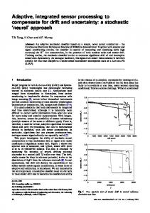
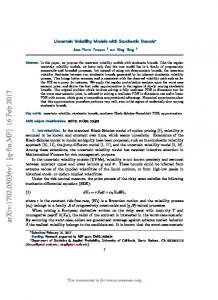
Figure 1: Graphical models to generate x1:T with a recurrent neural network (RNN) and a state space model (SSM). Diamond-shaped units are used for deterministic states, while circles are used for stochastic ones. For sequence generation, like in a language model, one can use ut = xt−1 .

latent states of the model, and allows us to improve inference by conveniently using the information coming from the whole sequence at each time step. The posterior distribution over the latent states of the SRNN is highly non-stationary while we are learning the parameters of the model. To further improve the variational approximation, we show that we can construct the inference network so that it only needs to learn how to compute the mean of the variational approximation at each time step given the mean of the predictive prior distribution. In Section 4 we test the performances of SRNN on speech and polyphonic music modeling tasks. SRNN improves the state of the art results on the Blizzard and TIMIT speech data sets by a large margin, and performs comparably to competing models on polyphonic music modeling. Finally, other models that extend RNNs by adding stochastic units will be reviewed and compared to SRNN in Section 5.

2

Recurrent Neural Networks and State Space Models

Recurrent neural networks and state space models are widely used to model temporal sequences of vectors x1:T = (x1 , x2 , . . . , xT ) that possibly depend on inputs u1:T = (u1 , u2 , . . . , uT ). Both models rest on the assumption that the sequence x1:t of observations up to time t can be summarized by a latent state dt or zt , which is deterministically determined (dt in a RNN) or treated as a random variable which is averaged away (zt in a SSM). The difference in treatment of the latent state has traditionally led to vastly different models: RNNs recursively compute dt = f (dt−1 , ut ) using a parameterized nonlinear function f , like a LSTM cell or a GRU. The RNN observation probabilities p(xt |dt ) are equally modeled with nonlinear functions. SSMs, like linear Gaussian or hidden Markov models, explicitly model uncertainty in the latent process through z1:T . Parameter inference in a SSM requires z1:T to be averaged out, and hence p(zt |zt−1 , ut ) and p(xt |zt ) are often restricted to the exponential family of distributions to make many existing approximate inference algorithms applicable. On the other hand, averaging a function over the deterministic path d1:T in a RNN is a trivial operation. The striking similarity in factorization between these models is illustrated in Figures 1a and 1b. Can we combine the best of both worlds, and make the stochastic state transitions of SSMs nonlinear whilst keeping the gated activation mechanism of RNNs? Below, we show that a more expressive model can be created by stacking a SSM on top of a RNN, and that by keeping them layered, the functional form of the true posterior distribution over z1:T guides the design of a backward-recursive structured variational approximation.

3

Stochastic Recurrent Neural Networks

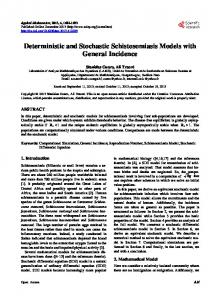
We define a SRNN as a generative model pθ by temporally interlocking a SSM with a RNN, as illustrated in Figure 2a. The joint probability of a single sequence and its latent states, assuming knowledge of the starting states z0 = 0 and d0 = 0, and inputs u1:T , factorizes as 2

xt−1

xt

xt+1

xt−1

xt

xt+1

zt−1

zt

zt+1

zt−1

zt

zt+1

dt−1

dt

dt+1

at−1

at

at+1

ut−1

ut

ut+1

dt−1

dt

dt+1

(a) Generative model pθ

(b) Inference network qφ

Figure 2: A SRNN as a generative model pθ for a sequence x1:T . Posterior inference of z1:T and d1:T is done through an inference network qφ , which uses a backward-recurrent state at to approximate the nonlinear dependence of zt on future observations xt:T and states dt:T ; see Equation (7).

pθ (x1:T , z1:T , d1:T |u1:T , z0 , d0 ) = pθx (x1:T |z1:T , d1:T ) pθz (z1:T |d1:T , z0 ) pθd (d1:T |u1:T , d0 ) =

T Y

pθx (xt |zt , dt ) pθz (zt |zt−1 , dt ) pθd (dt |dt−1 , ut ) .

(1)

t=1

The SSM and RNN are further tied with skip-connections from dt to xt . The joint density in (1) is parameterized by θ = {θx , θz , θd }, which will be adapted together with parameters φ of a so-called “inference network” qφ to best model N independently observed data sequences {xi1:Ti }N i=1 that are described by the log marginal likelihood or evidence X
X L(θ) = log pθ {xi1:Ti } | {ui1:Ti , zi0 , di0 }N log pθ (xi1:Ti |ui1:Ti , zi0 , di0 ) = Li (θ) . (2) i=1 = i

i

Throughout the paper, we omit superscript i when only one sequence is referred to, or when it is clear from the context. In each log likelihood term Li (θ) in (2), the latent states z1:T and d1:T were averaged out of (1). Integrating out d1:T is done by simply substituting its deterministically obtained value, but z1:T requires more care, and we return to it in Section 3.2. Following Figure 2a, the states d1:T are determined from d0 and u1:T through the recursion dt = fθd (dt−1 , ut ). In our implementation fθd is a GRU network with parameters θd . For later convenience we denote the value e t ), i.e. e 1:T . Therefore pθ (dt |dt−1 , ut ) = δ(dt − d of d1:T , as computed by application of fθd , by d d e 1:T . d1:T follows a delta distribution centered at d Unlike the VRNN [8], zt directly depends on zt−1 , as it does in a SSM, via pθz (zt |zt−1 , dt ). This split makes a clear separation between the deterministic and stochastic parts of pθ ; the RNN remains entirely deterministic and its recurrent units do not depend on noisy samples of zt , while the prior over zt follows the Markov structure of SSMs. The split allows us to later mimic the structure of the posterior distribution over z1:T and d1:T in its approximation qφ . We let the prior transition (p) (p) distribution pθz (zt |zt−1 , dt ) = N (zt ; µt , vt ) be a Gaussian with a diagonal covariance matrix, whose mean and log-variance are parameterized by neural networks that depend on zt−1 and dt , (p)

µt

(p)

(p)

= NN1 (zt−1 , dt ) ,

log vt

(p)

= NN2 (zt−1 , dt ) , (p) NN1

(3) (p) NN2 ,

where NN denotes a neural network. Parameters θz denote all weights of and which are two-layer feed-forward networks in our implementation. Similarly, the parameters of the emission distribution pθx (xt |zt , dt ) depend on zt and dt through a similar neural network that is parameterized by θx . 3.1

Variational inference for the SRNN

The stochastic variables z1:T of the nonlinear SSM cannot be analytically integrated out to obtain L(θ) in (2). Instead of maximizing L with respect to θ, we maximize a variational evidence lower 3

P bound (ELBO) F(θ, φ) = i Fi (θ, φ) ≤ L(θ) with respect to both θ and the variational parameters φ [18]. The ELBO is a sum of lower bounds Fi (θ, φ) ≤ Li (θ), one for each sequence i, ZZ pθ (x1:T , z1:T , d1:T |A) Fi (θ, φ) = qφ (z1:T , d1:T |x1:T , A) log dz1:T dd1:T , (4) qφ (z1:T , d1:T |x1:T , A) where A = {u1:T , z0 , d0 } is a notational shorthand. Each sequence’s approximation qφ shares parameters φ with all others, to form the auto-encoding variational Bayes inference network or variational auto encoder (VAE) [21, 26] shown in Figure 2b. Maximizing F(θ, φ) – which we call “training” the neural network architecture with parameters θ and φ – is done by stochastic gradient ascent, and in doing so, both the posterior and its approximation qφ change simultaneously. All the intractable expectations in (4) would typically be approximated by sampling, using the reparameterization trick [21, 26] or control variates [24] to obtain low-variance estimators of its gradients. We use the reparameterization trick in our implementation. Iteratively maximizing F over θ and φ separately would yield an expectation maximization-type algorithm, which has formed a backbone of statistical modeling for many decades [9]. The tightness of the bound depends on how well we can approximate the i = 1, . . . , N factors pθ (zi1:Ti , di1:Ti |xi1:Ti , Ai ) that constitute the true posterior over all latent variables with their corresponding factors qφ (zi1:Ti , di1:Ti |xi1:Ti , Ai ). In what follows, we show how qφ could be judiciously structured to match the posterior factors. We add initial structure to qφ by noticing that the prior pθd (d1:T |u1:T , d0 ) in the generative model e 1:T , and so is the posterior pθ (d1:T |x1:T , u1:T , d0 ). Consequently, we let is a delta function over d e 1:T as that of the generative the inference network use exactly the same deterministic state setting d model, and we decompose it as qφ (z1:T , d1:T |x1:T , u1:T , z0 , d0 ) = qφ (z1:T |d1:T , x1:T , z0 ) q(d1:T |x1:T , u1:T , d0 ) . | {z }

(5)

= pθd (d1:T |u1:T ,d0 )

This choice exactly approximates one delta-function by itself, and simplifies the ELBO by letting them cancel out. By further taking the outer average in (4), one obtains h i  

e 1:T ) − KL qφ (z1:T |d e 1:T , x1:T , z0 ) pθ (z1:T |d e 1:T , z0 ) , Fi (θ, φ) = Eqφ log pθ (x1:T |z1:T , d (6) e 1:T . The first term is an expected log likelihood which still depends on θd , u1:T and d0 via d e 1:T , x1:T , z0 ), while KL denotes the Kullback-Leibler divergence between two under qφ (z1:T |d distributions. Having stated the second factor in (5), we now turn our attention to parameterizing the first factor in (5) to resemble its posterior equivalent, by exploiting the temporal structure of pθ . 3.2

Exploiting the temporal structure

The true posterior distribution of the stochastic states z1:T , given Q both the data and the deterministic states d1:T , factorizes as pθ (z1:T |d1:T , x1:T , u1:T , z0 ) = t pθ (zt |zt−1 , dt:T , xt:T ). This can be verified by considering the conditional independence properties of the graphical model in Figure 2a using d-separation [14]. This shows that, knowing zt−1 , the posterior distribution of zt does not depend on the past outputs and deterministic states, but only on the present and future ones; this was also noted in [22]. Instead of factorizing qφ as a mean-field approximation across time steps, we keep the structured form of the posterior factors, including zt ’s dependence on zt−1 , in the variational approximation Y Y qφ (z1:T |d1:T , x1:T , z0 ) = qφ (zt |zt−1 , dt:T , xt:T ) = qφz (zt |zt−1 , at = gφa (at+1 , [dt , xt ])) , t

t

(7) where [dt , xt ] is the concatenation of the vectors dt and xt . The graphical model for the inference network is shown in Figure 2b. Apart from the direct dependence of the posterior approximation at time t on both dt:T and xt:T , the distribution also depends on d1:t−1 and x1:t−1 through zt−1 . We mimic each posterior factor’s nonlinear long-term dependence on dt:T and xt:T through a backwardrecurrent function gφa , shown in (7), which we will return to in greater detail in Section 3.3. The inference network in Figure 2b is therefore parameterized by φ = {φz , φa } and θd . In (7) all time steps are taken into account when constructing the variational approximation at time t; this can therefore be seen as a smoothing problem. In our experiments we also consider filtering, 4

where only the information up to time t is used to define qφ (zt |zt−1 , dt , xt ). As the parameters φ are shared across time steps, we can easily handle sequences of variable length in both cases. As both the generative model and inference network factorize over time steps in (1) and (7), the ELBO in (6) separates as a sum over the time steps h X   et) + Fi (θ, φ) = Eqφ∗ (zt−1 ) Eqφ (zt |zt−1 ,det:T ,xt:T ) log pθ (xt |zt , d t

 i

e t:T , xt:T ) pθ (zt |zt−1 , d et) , − KL qφ (zt |zt−1 , d

(8)

where qφ∗ (zt−1 ) denotes the marginal distribution of zt−1 in the variational approximation to the e 1:T , x1:T , z0 ), given by posterior qφ (z1:t−1 |d Z h i e 1:T , x1:T , z0 ) dz1:t−2 = Eq∗ (z ) qφ (zt−1 |zt−2 , d e t−1:T , xt−1:T ) . qφ∗ (zt−1 ) = qφ (z1:t−1 |d t−2 φ (9) We can interpret (9) as having a VAE at each time step t, with the VAE being conditioned on the past through the stochastic variable zt−1 . To compute (8), the dependence on zt−1 needs to be integrated out, using our posterior knowledge at time t − 1 which is given by qφ∗ (zt−1 ). We approximate the outer expectation in (8) using a Monte Carlo estimate, as samples from qφ∗ (zt−1 ) can be efficiently obtained by ancestral sampling. The sequential formulation of the inference model in (7) allows (s) (s) such samples to be drawn and reused, as given a sample zt−2 from qφ∗ (zt−2 ), a sample zt−1 from (s) e qφ (zt−1 |z , dt−1:T , xt−1:T ) will be distributed according to q ∗ (zt−1 ). t−2

3.3

φ

Parameterization of the inference network

The variational distribution qφ (zt |zt−1 , dt:T , xt:T ) needs to approximate the dependence of the true posterior pθ (zt |zt−1 , dt:T , xt:T ) on dt:T and xt:T , and as alluded to in (7), this is done by e t:T and xt:T backwards in time. Specifically, we initialize the hidrunning a RNN with inputs d den state of the backward-recursive RNN in Figure 2b as aT +1 = 0, and recursively compute e t , xt ]). The function gφ represents a recurrent neural network with, for examat = gφa (at+1 , [d a ple, LSTM or GRU units.QEach sequence’s variational approximation factorizes over time with qφ (z1:T |d1:T , x1:T , z0 ) = t qφz (zt |zt−1 , at ), as shown in (7). We let qφz (zt |zt−1 , at ) be a Gaussian with diagonal covariance, whose mean and the log-variance are parameterized with φz as (q)

µt

(q)

(q)

= NN1 (zt−1 , at ) ,

log vt

(q)

= NN2 (zt−1 , at ) .

(10)

Instead of smoothing, we can also do filtering by using a neural network to approximate the dependence of the true posterior pθ (zt |zt−1 , dt , xt ) on dt and xt , through for instance at = NN(a) (dt , xt ). Improving the posterior approximation. In our experiments we found that during training, the parameterization introduced in (10) can lead to small values of the KL term e t )) in the ELBO in (8). This happens when gφ in the inference KL(qφ (zt |zt−1 , at ) k pθ (zt |zt−1 , d network does not rely on the information propagated back from future outputs in at , but it is mostly e t to imitate the behavior of the prior. The inference network could therefore using the hidden state d get stuck by trying to optimize the ELBO through sampling from the prior of the model, making the variational approximation to the posterior useless. To overcome this issue, we directly include some knowledge of the predictive prior dynamics in the parameterization of the inference network, using our approximation of the posterior distribution qφ∗ (zt−1 ) over the previous latent states. In the spirit of sequential Monte Carlo methods [11], we improve the parameterization of qφ (zt |zt−1 , at ) by using qφ∗ (zt−1 ) from (9). As we are constructing the variational distribution sequentially, we approximate the predictive prior mean, i.e. our “best guess” on the prior dynamics of zt , as Z Z (p) (p) (p) b t = NN1 (zt−1 , dt ) p(zt−1 |x1:T ) dzt−1 ≈ NN1 (zt−1 , dt ) qφ∗ (zt−1 ) dzt−1 , (11) µ where we used the parameterization of the prior distribution in (3). We estimate the integral required (p) b t by reusing the samples that were needed for the Monte Carlo estimate of the ELBO to compute µ 5

in (8). This predictive prior mean can then be used in the parameterization of the mean of the variational approximation qφ (zt |zt−1 , at ), (q)

µt

(p)

bt =µ

(q)

+ NN1 (zt−1 , at ) ,

(12)

and we refer to this parameterization as Resq in the results Algorithm 1 Inference of SRNN with (q) in Section 4. Rather than directly learning µt , we learn Resq parameterization from (12). (q) (p) b t and µt . It is straightforward the residual between µ e 1:T and a1:T 1: inputs: d to show that with this parameterization the KL-term in 2: initialize z0 (p) (q) b t , but only on NN1 (zt−1 , at ). 3: for t = 1 to T do (8) will not depend on µ (p) (p) et) Learning the residual improves inference, making it seem- 4: µ b t = NN1 (zt−1 , d ingly easier for the inference network to track changes (q) (p) (q) b t + NN1 (zt−1 , at ) 5: µt = µ in the generative model while the model is trained, as it (q) (q) 6: log v = NN2 (zt−1 , at ) will only have to learn how to “correct” the predictive t (q) (q) prior dynamics by using the information coming from 7: zt ∼ N (zt ; µt , vt ) e dt:T and xt:T . We did not see any improvement in results 8: end for (q) by parameterizing log vt in a similar way. The inference procedure of SRNN with Resq parameterization for one sequence is summarized in Algorithm 1.

4

Results

In this section the SRNN is evaluated on the modeling of speech and polyphonic music data, as they have shown to be difficult to model without a good representation of the uncertainty in the latent states [3, 8, 12, 13, 16]. We test SRNN on the Blizzard [19] and TIMIT raw audio data sets (Table 1) used in [8]. The preprocessing of the data sets and the testing performance measures are identical to those reported in [8]. Blizzard is a dataset of 300 hours of English, spoken by a single female speaker. TIMIT is a dataset of 6300 English sentences read by 630 speakers. As done in [8], for Blizzard we report the average log-likelihood for half-second sequences and for TIMIT we report the average log likelihood per sequence for the test set sequences. Note that the sequences in the TIMIT test set are on average 3.1s long, and therefore 6 times longer than those in Blizzard. For the raw audio datasets we use a fully factorized Gaussian output distribution. Additionally, we test SRNN for modeling sequences of polyphonic music (Table 2), using the four data sets of MIDI songs introduced in [4]. Each data set contains more than 7 hours of polyphonic music of varying complexity: folk tunes (Nottingham data set), the four-part chorales by J. S. Bach (JSB chorales), orchestral music (MuseData) and classical piano music (Piano-midi.de). For polyphonic music we use a Bernoulli output distribution to model the binary sequences of piano notes. In our experiments we set ut = xt−1 , but ut could also be used to represent additional input information to the model. All models where implemented using Theano [2], Lasagne [10] and Parmesan1 . Training using a NVIDIA Titan X GPU took around 1.5 hours for TIMIT, 18 hours for Blizzard, less than 15 minutes for the JSB chorales and Piano-midi.de data sets, and around 30 minutes for the Nottingham and MuseData data sets. To reduce the computational requirements we use only 1 sample to approximate all the intractable expectations in the ELBO (notice that the KL term can be computed analytically). Further implementation and experimental details can be found in the Supplementary Material. Blizzard and TIMIT. Table 1 compares the average log-likelihood per test sequence of SRNN to the results from [8]. For RNNs and VRNNs the authors of [8] test two different output distributions, namely a Gaussian distribution (Gauss) and a Gaussian Mixture Model (GMM). VRNN-I differs from the VRNN in that the prior over the latent variables is independent across time steps, and it is therefore similar to STORN [3]. For SRNN we compare the smoothing and filtering performance (denoted as smooth and filt in Table 1), both with the residual term from (12) and without it (10) (denoted as Resq if present). We prefer to only report the more conservative evidence lower bound for SRNN, as the approximation of the log-likelihood using standard importance sampling is known to be difficult to compute accurately in the sequential setting [11]. We see from Table 1 that SRNN outperforms all the competing methods for speech modeling. As the test sequences in TIMIT are on average more than 6 times longer than the ones for Blizzard, the results obtained with SRNN for 1

github.com/casperkaae/parmesan. The code for SRNN is available at github.com/marcofraccaro/srnn.

6

Models

Blizzard

TIMIT

SRNN (smooth+Resq )

≥11991 ≥ 60550 ≥ 10991 ≥ 59269 ≥ 10572 ≥ 52126 ≥ 10846 ≥ 50524 ≥ 9107 ≥ 28982 ≈ 9392 ≈ 29604 VRNN-Gauss ≥ 9223 ≥ 28805 ≈ 9516 ≈ 30235 VRNN-I-Gauss ≥ 8933 ≥ 28340 ≈ 9188 ≈ 29639 RNN-GMM 7413 26643 RNN-Gauss 3539 -1900 Table 1: Average log-likelihood per sequence on the test sets. For TIMIT the average test set length is 3.1s, while the Blizzard sequences are all 0.5s long. The non-SRNN results are reported as in [8]. Smooth: gφa is a GRU running backwards; filt: gφa is a feed-forward network; Resq : parameterization with residual in (12). SRNN (smooth) SRNN (filt+Resq ) SRNN (filt) VRNN-GMM

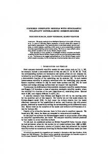
Figure 3: Visualization of the average KL term and reconstructions of the output mean and log-variance for two examples from the Blizzard test set.

Models Nottingham JSB chorales MuseData Piano-midi.de SRNN (smooth+Resq ) ≥ −2.94 ≥ −4.74 ≥ −6.28 ≥ −8.20 TSBN ≥ −3.67 ≥ −7.48 ≥ −6.81 ≥ −7.98 NASMC ≈ −2.72 ≈ −3.99 ≈ −6.89 ≈ −7.61 STORN ≈ −2.85 ≈ −6.91 ≈ −6.16 ≈ −7.13 RNN-NADE ≈ −2.31 ≈ −5.19 ≈ −5.60 ≈ −7.05 ≈ −4.46 ≈ −8.71 ≈ −8.13 ≈ −8.37 RNN Table 2: Average log-likelihood on the test sets. The TSBN results are from [13], NASMC from [16], STORN from [3], RNN-NADE and RNN from [4].

TIMIT are in line with those obtained for Blizzard. The VRNN, which performs well when the voice of the single speaker from Blizzard is modeled, seems to encounter difficulties when modeling the 630 speakers in the TIMIT data set. As expected, for SRNN the variational approximation that is obtained when future information is also used (smoothing) is better than the one obtained by filtering. Learning the residual between the prior mean and the mean of the variational approximation, given in (12), further improves the performance in 3 out of 4 cases. In the first two lines of Figure 3 we plot two raw signals from the Blizzard test set and the average KL term between the variational approximation and the prior distribution. We see that the KL term increases whenever there is a transition in the raw audio signal, meaning that the inference network is using the information coming from the output symbols to improve inference. Finally, the reconstructions of the output mean and log-variance in the last two lines of Figure 3 look consistent with the original signal. Polyphonic music. Table 2 compares the average log-likelihood on the test sets obtained with SRNN and the models introduced in [3, 4, 13, 16]. As done for the speech data, we prefer to report the more conservative estimate of the ELBO in Table 2, rather than approximating the log-likelihood with importance sampling as some of the other methods do. We see that SRNN performs comparably to other state of the art methods in all four data sets. We report the results using smoothing and learning the residual between the mean of the predictive prior and the mean of the variational approximation, but the performances using filtering and directly learning the mean of the variational approximation are now similar. We believe that this is due to the small amount of data and the fact that modeling MIDI music is much simpler than modeling raw speech signals. 7

5

Related work

A number of works have extended RNNs with stochastic units to model motion capture, speech and music data [3, 8, 12, 13, 16]. The performances of these models are highly dependent on how the dependence among stochastic units is modeled over time, on the type of interaction between stochastic units and deterministic ones, and on the procedure that is used to evaluate the typically intractable log likelihood. Figure 4 highlights how SRNN differs from some of these works. In STORN [3] (Figure 4a) and DRAW [15] the stochastic units at each time step have an isotropic Gaussian prior and are independent between time steps. The stochastic units are used as an input to the deterministic units in a RNN. As in our work, the reparameterization trick [21, 26] is used to optimize an ELBO. The authors of the VRNN [8] (Figure 4b) note that it is beneficial to add information coming from the past states to the prior over latent varizt−1 zt−1 zt zt zt ables zt . The VRNN lets the prior pθz (zt |dt ) over the stochastic units depend on the deterministic units dt , dt−1 dt−1 dt dt which in turn depend on both the deterministic and the stochastic units at ut ut ut the previous time step through the recursion dt = f (dt−1 , zt−1 , ut ). (a) STORN (b) VRNN (c) Deep Kalman Filter The SRNN differs by clearly separating the deterministic and stochastic Figure 4: Generative models of x1:T that are related to SRNN. part, as shown in Figure 2a. The sepaFor sequence modeling it is typical to set ut = xt−1 . ration of deterministic and stochastic units allows us to improve the posterior approximation by doing smoothing, as the stochastic units still depend on each other when we condition on d1:T . In the VRNN, on the other hand, the stochastic units are conditionally independent given the states d1:T . Because the inference and generative networks in the VRNN share the deterministic units, the variational approximation would not improve by making it dependent on the future through at , when calculated with a backward GRU, as we do in our model. Unlike STORN, DRAW and VRNN, the SRNN separates the “noisy” stochastic units from the deterministic ones, forming an entire layer of interconnected stochastic units. We found in practice that this gave better performance and was easier to train. The works by [1, 22] (Figure 4c) show that it is possible to improve inference in SSMs by using ideas from VAEs, similar to what is done in the stochastic part (the top layer) of SRNN. Towards the periphery of related works, [16] approximates the log likelihood of a SSM with sequential Monte Carlo, by learning flexible proposal distributions parameterized by deep networks, while [13] uses a recurrent model with discrete stochastic units that is optimized using the NVIL algorithm [23]. xt

6

xt

xt

Conclusion

This work has shown how to extend the modeling capabilities of recurrent neural networks by combining them with nonlinear state space models. Inspired by the independence properties of the intractable true posterior distribution over the latent states, we designed an inference network in a principled way. The variational approximation for the stochastic layer was improved by using the information coming from the whole sequence and by using the Resq parameterization to help the inference network to track the non-stationary posterior. SRNN achieves state of the art performances on the Blizzard and TIMIT speech data set, and performs comparably to competing methods for polyphonic music modeling.

Acknowledgements We thank Casper Kaae Sønderby and Lars Maaløe for many fruitful discussions, and NVIDIA Corporation for the donation of TITAN X and Tesla K40 GPUs. Marco Fraccaro is supported by Microsoft Research through its PhD Scholarship Programme.

8

References [1] E. Archer, I. M. Park, L. Buesing, J. Cunningham, and L. Paninski. Black box variational inference for state space models. arXiv:1511.07367, 2015. [2] F. Bastien, P. Lamblin, R. Pascanu, J. Bergstra, I. Goodfellow, A. Bergeron, N. Bouchard, D. Warde-Farley, and Y. Bengio. Theano: new features and speed improvements. arXiv:1211.5590, 2012. [3] J. Bayer and C. Osendorfer. Learning stochastic recurrent networks. arXiv:1411.7610, 2014. [4] N. Boulanger-Lewandowski, Y. Bengio, and P. Vincent. Modeling temporal dependencies in highdimensional sequences: Application to polyphonic music generation and transcription. arXiv:1206.6392, 2012. [5] S. R. Bowman, L. Vilnis, O. Vinyals, A. M. Dai, R. Jozefowicz, and S. Bengio. Generating sentences from a continuous space. arXiv:1511.06349, 2015. [6] K. Cho, B. Van Merriënboer, Ç. Gülçehre, D. Bahdanau, F. Bougares, H. Schwenk, and Y. Bengio. Learning phrase representations using RNN encoder–decoder for statistical machine translation. In EMNLP, pages 1724–1734, 2014. [7] J. Chung, C. Gulcehre, K. Cho, and Y. Bengio. Empirical evaluation of gated recurrent neural networks on sequence modeling. arXiv:1412.3555, 2014. [8] J. Chung, K. Kastner, L. Dinh, K. Goel, A. C. Courville, and Y. Bengio. A recurrent latent variable model for sequential data. In NIPS, pages 2962–2970, 2015. [9] A. P. Dempster, N. M. Laird, and D. B. Rubin. Maximum likelihood from incomplete data via the EM algorithm. Journal of the Royal Statistical Society, Series B, 39(1), 1977. [10] S. Dieleman, J. Schlüter, C. Raffel, E. Olson, S. K. Sønderby, D. Nouri, E. Battenberg, and A. van den Oord. Lasagne: First release, 2015. [11] A. Doucet, N. de Freitas, and N. Gordon. An introduction to sequential Monte Carlo methods. In Sequential Monte Carlo Methods in Practice, Statistics for Engineering and Information Science. 2001. [12] O. Fabius and J. R. van Amersfoort. Variational recurrent auto-encoders. arXiv:1412.6581, 2014. [13] Z. Gan, C. Li, R. Henao, D. E. Carlson, and L. Carin. Deep temporal sigmoid belief networks for sequence modeling. In NIPS, pages 2458–2466, 2015. [14] D. Geiger, T. Verma, and J. Pearl. Identifying independence in Bayesian networks. Networks, 20:507–534, 1990. [15] K. Gregor, I. Danihelka, A. Graves, and D. Wierstra. DRAW: A recurrent neural network for image generation. In ICML, 2015. [16] S. Gu, Z. Ghahramani, and R. E. Turner. Neural adaptive sequential Monte Carlo. In NIPS, pages 2611–2619, 2015. [17] S. Hochreiter and J. Schmidhuber. Long short-term memory. Neural Computation, 9(8):1735–1780, Nov. 1997. [18] M. I. Jordan, Z. Ghahramani, T. S. Jaakkola, and L. K. Saul. An introduction to variational methods for graphical models. Machine Learning, 37(2):183–233, 1999. [19] S. King and V. Karaiskos. The Blizzard challenge 2013. In The Ninth Annual Blizzard Challenge, 2013. [20] D. Kingma and J. Ba. Adam: A method for stochastic optimization. arXiv:1412.6980, 2014. [21] D. Kingma and M. Welling. Auto-encoding variational Bayes. In ICLR, 2014. [22] R. G. Krishnan, U. Shalit, and D. Sontag. Deep Kalman filters. arXiv:1511.05121, 2015. [23] A. Mnih and K. Gregor. Neural variational inference and learning in belief networks. arXiv:1402.0030, 2014. [24] J. W. Paisley, D. M. Blei, and M. I. Jordan. Variational Bayesian inference with stochastic search. In ICML, 2012.

9

[25] T. Raiko, H. Valpola, M. Harva, and J. Karhunen. Building blocks for variational Bayesian learning of latent variable models. Journal of Machine Learning Research, 8:155–201, 2007. [26] D. J. Rezende, S. Mohamed, and D. Wierstra. Stochastic backpropagation and approximate inference in deep generative models. In ICML, pages 1278–1286, 2014. [27] S. Roweis and Z. Ghahramani. A unifying review of linear Gaussian models. Neural Computation, 11(2):305–45, 1999. [28] C. K. Sønderby, T. Raiko, L. Maaløe, S. K. Sønderby, and O. Winther. How to train deep variational autoencoders and probabilistic ladder networks. arXiv:1602.02282, 2016.

A

Experimental setup

A.1

Blizzard and TIMIT

The sampling rate is 16KHz and the raw audio signal is normalized using the global mean and standard deviation of the traning set. We split the raw audio signals in chunks of 2 seconds. The waveforms are then divided into non-overlapping vectors of size 200. The RNN thus runs for 160 steps2 . The model is trained to predict the next vector (xt ) given the current one (ut ). During training we use backpropagation through time (BPTT) for 0.5 seconds, i.e we have 4 updates for each 2 seconds of audio. For the first 0.5 second we initialize hidden units with zeros and for the subsequent 3 chunks we use the previous hidden states as initialization. For Blizzard we split the data using 90% for training, 5% for validation and 5% for testing. For testing we report the average log-likelihood per 0.5s sequences. For TIMIT we use the predefined test set for testing and split the rest of the data into 95% for training and 5% for validation. The training and testing setup are identical to the ones for Blizzard. For TIMIT the test sequences have variable length and are on average 3.1s, i.e. more than 6 times longer than Blizzard. We model the output using a fully factorized Gaussian distribution for pθx (xt |zt , dt ). The deterministic RNNs use GRUs [7], with 2048 units for Blizzard and 1024 units for TIMIT. In both cases, zt is a 256-dimensional vector. All the neural networks have 2 layers, with 1024 units for Blizzard and 512 for TIMIT, and use leaky rectified nonlinearities with leakiness 13 and clipped at ±3. In both generative and inference models we share a neural network to extract features from the raw audio signal. The sizes of the models were chosen to roughly match the number of parameters used in [8]. In all experiments it was fundamental to gradually introduce the KL term in the ELBO, as shown in [5, 25, 28]. We therefore multiply a temperature β to the KL term, i.e. βKL, and linearly increase β from 0.2 to 1 in the beginning of training (for Blizzard we increase it by 0.0001 after each update, while for TIMIT by 0.0003). In both data sets we used the ADAM optimizer [20]. For Blizzard we use a learning rate of 0.0003 and batch size of 128, for TIMIT they are 0.001 and 64 respectively. A.2

Polyphonic music

We use the same model architecture as in the speech modeling experiments, except for the output Bernoulli variables used to model the active notes. We reduced the number of parameters in the model to 300 deterministic hidden units for the GRU networks, and 100 stochastic units whose distributions are parameterized with neural networks with 1 layer of 500 units.

2

2s·16Khz / 200 = 160

10