Short-Term Load Forecasting by Feed-Forward Neural Networks Saied S. Sharif1, James H. Taylor2, Department of Electrical and Computer Engineering, University of New Brunswick, Fredericton, NB, CANADA, E3B 5A3 E-mail: 1)
[email protected], 2)
[email protected] Abstract A feed-forward neural network (FNN) is presented for the hourly load forecasting of the coming days. In this approach, 24 independent networks are used for the next day load forecast. Each network is utilized for the prediction of load at a specific hour - one network for hour one, one for hour two, and so on. The load forecast results of these networks are compared with the current New Brunswick (NB) Power load forecast program (a conventional time series package). Both programs are utilized to predict the hourly load of one day ahead. Totally 136 days are simulated. Based on simulation results, the FNN approach provides a better performance than the NB power program.
1. Introduction The term short-term load forecasting (STLF) is used for the prediction of the power system load over an interval ranging from one hour to one week. The first application of STLF is to drive the scheduling functions that determine the most economic commitment of generation sources. This scheduling applies to purely hydro systems, purely thermal systems, and mixed hydro/thermal systems. In general terms, computer programs for STLF involve tuning, adapting or training a mathematical model to fit historical data with minimal error, then using that model with forecast weather data, etc., to predict the future load level. STLF models can be divided into four main categories: a) conventional methods, including time series or regression models, b) fuzzy logic models, c) artificial neural network models, and d) expert system load forecasters. Within each category there are different approaches, architectures
and algorithms that may substantially impact performance. Artificial neural networks (ANNs) have shown superior performance in recent studies [2]-[9]. Different types of ANNs including supervised and unsupervised networks are proposed in the literature. Supervised networks including recurrent [2], and feed-forward [3][9] networks have attracted more attention than unsupervised networks [3]. In this paper, a novel feedforward neural network (FNN) is introduced. Based on preliminary results, separate FFNs for load forecast of each hour of the day have given better performance than one FNN for all the 24 hours. For this reason, 24 independent networks are used to predict the hourly load of the next day. For each network, a comprehensive set of input variables was tested, and the inputs with the best performance index were selected. The range of training data set was also adjusted to obtain the best results. A new performance index based on the daily energy forecast error for mixed hydro/thermal units is introduced. The organization of the paper is as follows: in Section 2, the basic concepts related to feed-forward neural networks are described. In Section 3, the architecture of input, hidden, and output layers are discussed. In Section 4, the prediction performance of the neural network is evaluated. In Section 5, the simulation results of the FNN and the existing NB Power program are compared, and concluding remarks are given in Section 6.
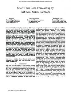
2. Neural network structure A multi-layer feed-forward neural network (FNN) can be used for STLF purposes. The FNN is trained to approximate the nonlinear function Fs(.) between the hourly load and the input variables. The FNN comprises a layer of input units, one or more hidden layer(s) and a layer of output units. An FNN with one hidden layer is
shown in Figure 1. The input layer consists of Ni inputs. Each ith input is connected to the each jth unit of the hidden layer by a weighting factor, Wij. Each unit in the hidden layer, called a neuron, performs a nonlinear transformation of its weighted input signals. The model of unit j (neuron j) in the hidden layer is shown in Figure 2. The output of this neuron can be formulated as: A j f h (net j ), (1) where fh is a nonlinear activation function in the hidden layer, and netj can be formulated as: Ni
net j Wij xi b j ,
(2)
i 1
Where xi is the input of unit i in the input layer; Wij is the weighting factor between neuron i of the input layer and neuron j of the hidden layer, respectively; and bj is the bias term of the neuron (a constant term). All the weighting factors and bias terms are adjusted during the training process. Input Hidden Output Layer Layer Layer Wij
xi
Wjk
yk
Nh
net k W jk A j bk ,
(4)
j 1
and Wjk is the weighting factor between neuron j in the hidden layer and neuron k in the output layer.
3. Neural network architecture The number of inputs, hidden layers, neurons in hidden layers, and outputs usually defines the FNN architecture. In this paper, 24 independent FNNs are utilized to forecast the hourly load of the next day. Each network is used for the prediction of the load at a specific hour - one network for hour one, one for hour two, and so on. The 24 FNNs are implemented in MetrixND, a neural network package [4]. Most of the inputs of these networks are the same, and can be divided into three main categories: a) calendar variables, b) weather variables, and c) load variables. These inputs, and the architecture of hidden and output layers are explained in the following sections. x1 . W1j . netj Aj xi Wij Slope
. . Summation Unit xNi WNij
. .
. .
. .
Nonlinear Activation Function Figure 2: The model of neuron j in the hidden layer
3.1. Inputs related to calendar variables j=1 to Nh k=1 to No i=1 to Ni Figure 1: A feed-forward neural network with one hidden layer The activation function, fh, can be a bounded monotonic function such as hyperbolic tangent, sigmoid, signum, semi-linear, etc., and in the training process, only the value of its slope is varied (see Figure 2). The structure of the FNN output layer is similar to the hidden layer with the exception that the inputs of the output layer are the outputs of the hidden layer. The output of neuron “ k ” in the output layer can be formulated as: yk f o (netk ), (3) where fo is the nonlinear activation function in the output layer, netk is equal to:
The Calendar variables which have the most impact on the load demand are: 1) the time of the day, 2) the day of the week, 3) the day of the year, 4) Holidays, 5) days near Holidays, 6) season, 7) sunrise and sunset times or daylight duration, and 8) the time change related to the daylight saving. Most of the calendar variables of FNN are represented by binary variables. These variables are described below. a) The day of the week: The day of the week is shown by seven different binary variables instead of one integer variable varying from one to seven [2]. b) Holidays: One binary variable is used for specifying the holidays. If a given day is a regular weekday or weekend, this variable is zero; otherwise it
gets assigned the value of one, which represents a holiday. c) Days near holidays: One continuous variable between zero and one is selected for representing the days near holidays such as the days around Christmas and New Year day. The value of this variable is selected by comparing the historical load of that day with a similar regular day. This input is set to zero if there is no major difference, and to one if there is large difference. d) Season: Four continuous variables between zero and one are dedicated for the four seasons of Spring, Summer, Fall, and Winter. For example, the value of one for Spring shows that the given day is in Spring. For a day like March 10th, the Winter variable is set equal to 0.8 and the Spring variable is set equal to 0.2. e) Daylight duration: The time difference between sunset and sunrise, which gives the daylight duration, is used as one continuous input variable. f) Daylight saving: One binary variable is used for daylight saving. This value is 0 for regular times and 1 for changed times. g) The day of the year: One continuous input variable is dedicated to the day of the year. This variable shows that the given day is which day in a year, and for a regular year varies between 1/365 and 1.
3.2. Inputs related to the weather variables The available historical weather data for the NB Power network are: 1) dry bulb temperature, 2) humidity, 3) wind speed, and 4) opacity or cloud coverage. All of these variables are described below. a) Dry bulb temperature: Several dry bulb temperatures are used as input variables. These temperatures are related to: 1) the forecast hour, 2) one hour before the forecast hour, 3) the forecast hour of one and two days before, 4) one hour in the morning of one day before, 5) one hour in the afternoon of one day before, 6) the minimum and maximum temperature of the forecast day, and 7) the minimum and maximum temperature of one and two days before the forecast day. The effect of comfort zone temperature on the load consumption is modeled by the following nonlinear transformation:
TC min T T 0 T T C max ^
T TC min
for
for TC min T TC max (5),
minimum and maximum temperatures for the comfort zone, respectively. b) Humidity: The selected FNN input variables related to humidity are: 1) the hourly humidity of the given hour, 2) the daily minimum and maximum humidity. c) Wind speed: The wind speed of the given hour is selected as another input of FNN. d) Opacity or cloud coverage: The FNN inputs related to opacity are: 1) the hourly opacity of the given hour, 2) the daily minimum and maximum opacity.
3.3. Inputs related to historical load data These data consist of actual hourly loads before the forecast day. The hourly load of the forecast day are most highly correlated to the load of one day, two days, seven days, and eight days before [5]. The selected hourly load data are discussed below. a) The load data of one hour before: If the actual load data of one hour before is not available, the load forecast of that hour will be used. b) The load of one day before at the same hour: The load of one day before at the same hour is used as an input variable regardless of the type of the previous day (weekday, weekend, or holiday). c) The load of two days before at the same hour d) The load data of one day before in the morning: One hourly historical load data of one day before in the morning (say hour 8) is selected as another input variable. e) The load data of one day before in the afternoon: One hourly historical load data of the previous day in the afternoon is also selected as another input.
3.4. Architecture of the hidden layer Each FNN has only one hidden layer. The number of neurons in this layer is equal to four. Other numbers of neurons, e.g., 3, 5, and 6 did not improve the load forecast accuracy. Two types of activation functions, sigmoid and semi-linear, were tested. The sigmoid activation function gave better results, and thus was selected as a candidate.
T TC max
for ^
where T is the actual temperature; T is the transformed temperature; and TCmin and TCmax are the related
3.5. Architecture of the output layer The output variable of each FNN is the hourly load forecast of the next day, yk, for k=1, 2, . . . , 24. Several
architectures have been proposed, and studied. Between them: 1) one FNN with 24 outputs for 24 hours [6], 2) seven networks, each for the 24 hours of one day of the week [7], and 3) 24 separate FNNs, each for one hour [8], can be cited. In this paper, the third approach has been utilized due to its superior performance.
4. Evaluation of prediction performance An important step in the design procedure of the neural network is the evaluation of forecasting performance. In general, the performance index is a measure of the load prediction error on an independent data set. The load forecast error should be in an acceptable range if the neural network is trained correctly, and if the training data set is representative of the forecasting period. The selection of appropriate training data sets and performance indices are discussed in the following sections.
where LF is the forecast load, LA is the actual load, n is the number of data point in the data set, and N is the total number of data points. The mean absolute percentage error, , can be formulated as:
1 N
| Ln F Ln A | * 100. Ln A n 1 N
(7)
Another index, which has practical importance in mixed hydro/thermal systems, is the daily energy forecast error. In general, for hourly generation scheduling of hydro/thermal units, the total generation cost is minimized. This minimization is based on the load forecast of the next hour and the available energy from hydro units. In many cases, the available energy from hydro units is specified for the whole day, and their hourly energy generations are not important as long as their daily energy generations meet the scheduled value. As a result, hydro unit generation can compensate some parts of the hourly load forecast error. The uncompensated part is related to the energy forecast error, which can be formulated as: 24
d ( Ln F Ln A ),
4.1. Selection of training data sets
(8)
n 1
In the training procedure, the parameters of the neural network are optimized based on available data. The accuracy of a subsequent load forecast is mainly dependent on the closeness of the training data and the selected time period for the load forecast. For this reason, several approaches for the selection of training data set have been proposed in the literature. In [6], three years of historical data are selected for training the neural network, to obtain good generalization. The load pattern in each year is strongly dependent on the weather conditions during that year. The neural network can be trained weekly or even monthly. In this paper, only sixteen months of historical data has been chosen. This window is selected after studying the weather pattern during the last several years.
4.2. Performance indices Several measures of forecast accuracy have been proposed as the performance index [9]. In this study, the two most commonly adopted for load forecast evaluation were used: 1) variance, ; and 2) mean absolute percentage error (MAPE); which can be formulated as follows: 2
2
1 N
N
(L
n
n 1
F
Ln A ) 2 ,
(6)
where
d
is the daily energy forecast error. The
daily energy forecast percentage error,
dp , can also be
used as an index for prediction performance, and formulated as: 24
(L
n
dp
F
Ln A )
n 1
*100
24
L
n
(9)
A
n 1
5. Simulation results The simulation results related to the FNN are discussed in this section. As mentioned before, the neural network was trained with sixteen months of historical data. The training data set covers the period of September 1997 through December 1998. After training the neural network, the FNN is used for a load forecast study of 136 days from January 1st to May 16th 1999. Load forecast results of the 24 FNNs are compared with the load forecast results of the existing NB Power program [10] (a conventional time series load forecast package). In both cases, the actual weather variables are used instead of forecast weather parameters. Load forecast results of the two programs for the specified study period are shown in Table 1. In column one, the
hour number of day is shown. Column two and three give the mean absolute percentage error (MAPE) of hourly load forecast for NB Power program and neural network approach, respectively. Based on these results, the performance of FNN for all the 24 hours is better than that from the NB Power package, and its MAPE of load forecast for all the 24 hours, 2.72%, is less than 70% of that from the NB Power program, 3.96%. Table 1: Load forecast error of the NB Power program and the neural network approach MAPE(HLF)+ NB FNNs Power 1 3.32 1.38 2 3.4 1.57 3 3.46 1.68 4 3.5 1.87 5 3.38 2.12 6 3.34 2.31 7 3.69 2.59 8 3.66 2.71 9 3.43 2.8 10 3.98 2.79 11 4.31 2.8 12 4.81 3.07 13 5.03 2.89 14 5.13 3.22 15 5.51 3.39 16 5.34 3.46 17 5.06 3.48 18 4.4o 3.53 19 4.03 3.33 20 3.71 3.02 21 3.56 2.78 22 3.04 2.79 23 2.89 2.88 24 3.02 2.97 Average 3.96 2.72 +:mean absolute percentage error of hourly load forecast The load forecast results of the two methods are also presented in Figure 3. In this figure, the MAPEs of load forecast for all the 136 days are compared. Energy forecast errors of the two programs for the study period are compared in Table 2. The values of this table are calculated as follows: 1) first by using Equation (9), the percentage energy error for each day is computed, and 2) the average absolute values of these errors are calculated over each day of the week. The calculated values for the NB Power and FNN programs are given in column two and three of Table 2, respectively. Based on these results, FNN has a lower
MAPE of daily energy forecast than that from the NB Power program for all the weekdays. The MAPE of daily energy forecast for all the days of FNN is 1.93%. This value is nearly 40% less than that from the NB Power package, 3.18%. The daily energy forecast results of the two methods are also presented in Figures 4 and 5. In these figures, the mean absolute daily energy forecast error for one weekday (Monday) and one weekend day (Sunday) are shown. " Average Actual Load in MW "
Hour No.
Actual Load in MW
1700 1600 1500 1400 1300 1200 1100 0
5
10 15 Time in Hour
20
25
Load Forecast Error in MW
MAPE of Load Forecast for " FNN = __ " and " NB Power = -- " 80 60 40 20 0 0
5
10 15 Time in Hour
20
25
Figure 3: Comparison of MAPE of load forecast Table 2: The energy forecast error of the NB Power and neural network programs Week Day Mondays Tuesdays Wednesdays Thursdays Fridays
MAPE(DEF)+ NB Power FNN 3.15 1.85 3.03 1.56 3.23 1.77 3.04 1.87 3.34 2.16
Saturdays Sundays Average
2.96 3.49 3.18
2.2 2.07 1.93
+: Mean absolute percentage error of daily energy forecast. " F N N = _ _ _ " , " N B P o w e r = -- " 14
MAPE OF ENERGY FORECAST
12
M A P E o f E n e rg y F o re c a s t fo r M o n d a y s F N N = 1.8 5, N B P ow er = 3.15
10
8
6
4
2
0
0 5 10 15 20 W E E K N U M B E R F R O M JA N U A R Y 1 9 9 9
Figure 4: Comparison of MAPE of daily energy forecast for Mondays " F N N = _ _ _ " , " N B P o w e r = -- "
6. Conclusion A set of 24 feed-forward neural networks is proposed to reduce the hourly load forecast error of the next day. In this method, 24 independent networks are utilized to predict the load of the next 24 hours. The input variables of FNN are selected from three important categories: a) calendar variables, 2) weather variables, and 3) load data variables. The range of training data set is adjusted to obtain the best performance indices. A new performance index based on the daily energy forecast error for mixed hydro/thermal units is introduced, MAPE(DEF). The load and energy forecast results of the FNN method are compared with the current NB Power load forecast program. By studying the weather pattern of the last several years, sixteen months of historical data was selected to train the neural network. The hourly load of one day ahead by using the actual weather data is predicted. Totally 136 days were simulated. Based on simulation results, the FNN approach has reduced the MAPE of hourly load forecast by more than 30% in comparison to the NB Power program. The FNN method also reduced the daily energy forecast MAPE that was 40% less than that from the NB Power program.
7. References
14
MAPE OF ENERGY FORECAST
12
M A P E o f E n e rg y F o re c a s t fo r S u n d a y s F N N = 2.07, N B P O W E R = 3.49
10
8
6
4
2
Figure 5: Comparison of MAPE of daily energy forecast for Sundays
[1] G. Gross, F.D. Galiana, “Short-Term Load Forecasting,” Proceedings of the IEEE, vol. 75, no. 12, Dec. 1987, pp. 1558-1573. [2] J. Vermaak, E.C. Botha, “Recurrent Neural Networks for Short- Term Load Forecasting,” IEEE Trans. PWRS, vol. 13, no. 1, Feb. 1998, pp. 126-132. [3] A. Piras, A. Germond, B. Buchenel, K. Imhof, Y. Jaccard, “Heterogeneous Artificial Neural Network for Short Term Electrical Load Forecasting,” IEEE Trans. PWRS, vol. 11, no. 1, Feb. 1996, pp. 397-402. [4] MetrixND, Regional Economic Research Inc., 11236 El Camino Real San Diego, California 92130-2650, USA. [5] K.Y. Lee, Y.T. Cha, J.H. Park, “Short-Term Load Forecasting Using an Artificial Neural Network,” IEEE Trans. PWRS, vol. 7, no. 1, Feb. 1992, pp. 124-132. [6] S.J. Kiartzis, C.E. Zoumas, J.B. Theocharis, A.G. Bakirtzis, V. Petridis, “Short-Term Load Forecasting in an Autonomous Power System Using Artificial Neural Networks,” IEEE Trans. PWRS, vol. 12, no. 4, Nov. 1997, pp. 1591-1596. [7] A.G. Bakirtzis, B. Petridis, S.J. Kiartzis, M.C. Alexladls, A.H. Malssis, “A Neural Network Short Term Load Forecasting Model for the Greek Power System,” IEEE Trans. PWRS, vol. 11, no. 2, May 1996, pp. 858-863. [8] P.K. Dash, H.P. Satpathy, A.C. Liew, S. Rahman, “A Real-Time Short-Term Load Forecasting Using
Functional Link Network,” IEEE Trans. PWRS, vol. 12, no. 2, May 1997, pp. 675-680. [9] T.W.S. Chow, C.-T. Leung, “Nonlinear Autoregressive Integrated Neural Network Model for Short-Term Load Forecasting,” IEE Proc. Generation Transmission Distribution, vol. 143, no. 5, Sep. 1996, pp. 500-506. [10] S. Cham, Abstract on Short Term Load Forecasting Method, NB Power Publication, 1990, pp. 2-1 to 2-24.