In the vicinity of a signal discontinuity, large wavelet coefficients can be generated. When these coefficients are quantized or lost, Gibbs-like phenomenon can be ...
THIS PAPER APPEARS IN IEEE TRANSACTIONS ON IMAGE PROCESSING, VOL. 16, ISSUE 1, JAN. 2007, P.46 - 56
1
Signal and Image Approximation using Interval Wavelet Transform Wei Siong Lee, and Ashraf A. Kassim, Member, IEEE
Abstract In signal approximation, classical wavelet synthesis are known to produce Gibbs-like phenomenon around discontinuities when wavelet coefficients in the cone of influence of the discontinuities are quantized. By analyzing a function in a piecewise manner, filtering across discontinuities can be avoided. Using this principle, the interval wavelet transform can generate sparser representations in the vicinity of discontinuities than classical wavelet transforms. This work introduces two new constructions of interval wavelets and shows how they can be used for image compression and upscaling. Index Terms wavelets on the interval, boundary filters, image approximation.
I. I NTRODUCTION
I
T is well known that wavelets can provide sparse, and hence efficient, representations of smooth functions. This property is especially advantageous to signal coding. In the vicinity of a signal discontinuity, large wavelet coefficients can be generated. When these coefficients are quantized or lost, Gibbs-like phenomenon can be observed in reconstructed signals. The problem worsens in the presence of higher dimensional discontinuities. For example in image compression, artifacts marked by softness, ringings, halos and color bleeding can be seen along edges. To overcome this inadequacy of classical wavelets, several techniques have been proposed for more efficient analysis and synthesis of singularity structures. For example, in [1][2][3][4][5][6], directionality is introduced into existing 2D wavelet functions. Separable 2D wavelets gives only 3 orientations in the decomposition subbands — vertical, horizontal and diagonal. Thus, edges with other orientation profiles will tend to have wavelet coefficients that span across all the subbands. By having directionality in wavelet bases, the wavelet coefficients for any edge can be contained in only one subband depending its orientation. Other works such as wavelet footprints [7][8], wavelet modulus maximas [9][10] and the Essentially Non-Oscillatory (ENO) wavelets [11] attempt to obtain sparser representations of 1D discontinuities. By using a dictionary containing normalized wavelet coefficient sets belonging to the same cone of influence of some discontinuities, the wavelet footprints technique is able provide compact representations of discontinuities through dictionary indices. Wavelet maximas are wavelet coefficients that are strict local maximums on the decomposition map. Meyer [12] and Berman [13] show that, by imposing minimum oscillation constraints on image reconstruction from the maximas, edge artifacts can be avoided. The ENO schemes [14][15] used in fluid dynamics to capture shocks, rarefaction and contact discontinuities, are applied in the ENO-wavelet transform to avoid filtering across discontinuities. This extrapolation approach is similar to [16] and [17]. Other approaches to construct orthonormal bases for analyzing 2D discontinuities include beamlets [18], wedgelets [19] and platelets [20]. The objective of this work is to show that more efficient edge representation can be obtained using interval wavelet transform. Given an ordered set of M + 1 breakpoints: K = {k0 , k1 , . . . , kM : k0 = 0, kM = N },
(1)
Fig. 1. An interval wavelet decomposition example on sequence X with breakpoints {k0 , k1 , k2 , k3 }. Each interval Xn are wavelet transformed to obtain their respective low Cn and high-pass Dn coefficients. If Xn is sufficiently smooth, Dn will be negligible.
2
Fig. 2.
THIS PAPER APPEARS IN IEEE TRANSACTIONS ON IMAGE PROCESSING, VOL. 16, ISSUE 1, JAN. 2007, P.46 - 56
Type I (dashed), Type II (black) and Type III (gray) boundary scaling φ and wavelet ψ functions based on symmlets (p = 4).
a N -length sequence X can be viewed as a cascade of M intervals, X =
{x0 , x1 , . . . , xN −2 , xN −1 }
=
{X0 , X1 , . . . , XM−1 }
(2)
where Xn = {xi }kn ≤i