Then, a Markov chain is constructed to move across these spaces, with the hope that the fast mixing of transitions ... The distribution is shown on the top left panel of Figure 1. -5. 0. 5. 10. -5. 0. 5. 10. -5. 0 .... time at each state of I. This procedure may be called marginal sintering. Simulated ..... x00 = (x0); and finally, (c) draw. 0.
BAYESIAN STATISTICS 6, pp. 000--000 J. M. Bernardo, J. O. Berger, A. P. Dawid and A. F. M. Smith (Eds.) Oxford University Press, 1998
Simulated Sintering: Markov Chain Monte Carlo With Spaces of Varying Dimensions JUN S. LIU1 and CHIARA SABATTI Stanford University, USA SUMMARY In an effort to extend the tempering methodology, we propose simulated sintering as a general framework for designing Markov chain Monte Carlo algorithms. To implement sintering, one identifies a family of probability distributions, all related to the target one and defined on spaces of different dimensions. Then, a Markov chain is constructed to move across these spaces, with the hope that the fast mixing of transitions in lower-dimensional spaces facilitates the simulation from the target distribution. Two types of sintering are discussed: conditional sintering, which is motivated by the multigrid Monte Carlo idea and can be regarded as a generalization of the Gibbs sampler; and marginal sintering, which can be achieved by reversible jump MCMC. To help mixing in a reversible jump MCMC algorithm, we suggest incorporating the dynamic weighting method proposed by Wong and Liang. Examples in graphical modeling and computational biology illustrate how these techniques can be applied. Keywords:
ALIGNMENT; CLASSIFICATION; DYNAMIC WEIGHTING, GIBBS SAMPLING; GRAPHICAL MODEL; MODEL SELECTION; MULTIGRID MONTE CARLO; REVERSIBLE JUMP; SIMULATED TEMPERING; TRANSFORMATION GROUP.
1. INTRODUCTION 1.1. Prelude Markov chain Monte Carlo (MCMC) has grown to be a standard tool for statistical computing. It is arguably the main driving force behind the recent surge of interest in computationally-intensive areas such as probabilistic expert system and graphical modeling (Lauritzen, 1996); Bayesian CART (Chipman et al., 1997); neural network training (Neal, 1996); classification and mixture models (Green, 1995); and nonparametric Bayes (Bush and MacEachern, 1996). In many complicated problems, however, slow-mixing of the Markov chain produced by a standard MCMC recipe still posts the greatest challenge. To overcome this difficulty, many techniques have been proposed, among which simulated tempering (Marinari and Parisi, 1992; Geyer and Thompson, 1995) is particularly interesting. Suppose � (x) is the target distribution. In simulated tempering, one builds a distribution family � whose members differ by one parameter, the temperature, and � corresponds to the ‘‘coldest’’ member of the family. Within �, one finds members that induce fast-mixing Markov chains and can be used to improve the simulation of � . The tempering methodology is very powerful, but its current implementation is somewhat limited. 1
Partially supported by NSF grant DMS 95-96096 and the Terman fellowship from Stanford University. Part of the manuscript was prepared when Liu was visiting Department of Mathematics, National University of Singapore; and Department of Statistics, University of California, Los Angeles.
2
Liu and Sabatti
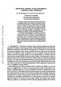
1.2. A simple illustration To illustrate the basic idea of simulated tempering and one of its potential problems, we consider a target distribution � which is a discretized mixture of two bivariate normal densities with the modes separated by more than 10 standard deviations. The distribution is shown on the top left panel of Figure 1.
10
10 5
5
10 5
0
10
-5
5
0
0
0
-5
-5
-5
10
10 5
5
10
10
0
-5
5
0
5
0
0
-5
-5
-5
10
10
5
5
10
0
-5
0
-5
10 5
0
5
0
-5
-5
Figure 1. Simulated tempering and simulated sintering. The normal distributions originating the mixtures have means (-5,5) and (5,-5). On the left hand side, from the top to the bottom, the value of the variance is 1, 4, 10. On the right hand side, � = 1, but the cardinality of the sample space is 64 � 64, 16 � 16 and 4 � 4.
Suppose one tries to sample from � by a Metropolis algorithm (Metropolis et al., 1953) with the nearest-neighbor simple random walk as the proposal chain. It is easily seen that such a sampler always gets stuck in one of the modes. As shown in the left panels of Figure 1, simulated tempering can be used to overcome the difficulty. In particular, we can build the distribution family � as � = f�0 ; �1 ; �2 g, where
�i = 12 N [(?5; ?5); �i 1] + 21 N [(5; 5); �i 1]; 2
2
with
� = 1; � = 4; � = 10: 2 0
2 1
2 2
Note that �0 corresponds to the target � . A MCMC algorithm can be designed (Geyer and Thompson, 1995) to draw (x; I ) from the distribution � � (x; I ) / f (I )�I (x), where f (I ) can be adjusted. Once convergence is reached, those x’s associated with I = 0 follow the distribution � .
3
Simulated Sintering
It is clear that in the hottest distribution (i.e., �2 ) the separation of the two modes is greatly reduced and the same Metropolis algorithm can be applied to draw from �2 without difficulty. However, by implementing the tempering suggestion, the Markov chain tends to spend too much time in uninteresting regions around (0,0), losing the advantage of MCMC over a simple random sampling approach. This problem becomes more serious as the dimension of the space increases. Other potential drawbacks of tempering are discussed in Liu and Sabatti (1998). On the right panel of Figure 1, we show an alternative solution to the problem. Instead of varying one parameter, i.e., the variance of the system, we change the accuracy used in describing the underlying phenomena. As can be intuitively seen, this overcomes the problem of bi-modality and also avoids the curse of dimensionality encountered by simulated tempering. 1.3. Outline of the article In this article, we explore possible generalizations of the tempering procedure along the line proposed by Wong (1995). More precisely, we consider the construction of the distribution family � with spaces of varying dimensions. We call this method simulated sintering. As tempering, sintering is a metallurgical technique: it consists of a combination of chemical reactions and temperature manipulation and is used to obtain a uniform piece of metal from an agglomerate of metal powder and plastic compounds. Because it implies the fractioning of the object of interest in smaller portions, we feel that it is a good metaphor for the procedures explored in this article. There are two main tasks in realizing simulated sintering: to find/construct the distribution family � = f�i g, and to design effective moves between the family members. The multigrid Monte Carlo (MGMC) provides a means to accomplish both of these tasks: it constructs the members of � and describes the moves between them via appropriate conditional and marginal distributions of � . In a sense, it is a generalized Gibbs sampler, but with the conditional distributions sequentially built up by the multigrid heuristics. Because the procedure uses conditional distributions exclusively, we call this construction conditional sintering. It is also of interest to construct the family � more freely by using approximations of �(x) at different resolution levels. For example, we can let � = f�j (x[j]); j = 0; 1; : : :; kg, where �0 = � and x[j ] is a dj -dimensional vector with d0 � d1 � � � � � dk . Then a reversible jumping rule (Green, 1995) can be designed to draw (x[I ] ; I ) from � � (x[I ] ; I ) / f (I )�I (x[I ] ), where I = 0; 1; : : :; d. The coefficient f (I ) is adjusted to make the chain spend about equal time at each state of I . This procedure may be called marginal sintering. Simulated tempering can be seen as a special marginal sintering. As noted by Green (1995), dimension-change occurs naturally in Bayesian model selection problems, image segmentations, change-point problems, etc. In these situations, members of the family � are naturally induced by the problem (e.g., the posterior distribution of the parameters under each model type). Thus, the MCMC algorithm involved in such problems is also a marginal sintering, in which prominent difficulty is in the construction of efficient moves between the family members. Green (1995) gives explicit rules to guide for the choice of proper proposals for jumping across different dimensional spaces. When applying the rules in a difficult problem, however, we found that acceptance probability for the jump can be extremely small: thus, the resulting Markov chain mixes very slowly. To cope with the difficulty, we propose to use the dynamic weighting method of Wong and Liang (1997) to help for space-jumping. In dynamic weighting, a weight variable is associated with the Markov chain sampler so as to let the chain move across low-probability barriers more freely. The weights can later be used to correct the bias. This article is organized as follows: Section 2 presents the group move in MCMC and
4
Liu and Sabatti
conditional sintering; Section 3 describes dynamic weighting and discusses how to use it in marginal sintering; Section 4 gives an example of graphical model selection; Section 5 outlines an algorithm for protein sequence alignment and classification; Section 6 shows an improved algorithm for inference with multivariate t-distribution; and Section 7 concludes with a brief discussion. 2. MULTIGRID MONTE CARLO APPROACH 2.1. Gibbs Sampler and Beyond Suppose X is the space on which � is defined. Let x = (x1 ; : : :; xd ) be a point in this space. The Gibbs sampler (Gelfand and Smith, 1990) is an effective method for reducing a high dimensional simulation problem to a lower dimensional one --- via using conditional distributions (it is important to realize that there are methods other than reversible jump for traversing different dimensional spaces). In Gibbs sampling, one randomly or systematically choose a coordinate, say x1 , and then update it with a new sample x01 drawn from a conditional distribution --- � (� j x[?1]), where x[?A] refers to (xj ; j 2 Ac ) for any subset A of the coordinates. A simple restatement of this procedure can be potentially useful: the update can be seen as a random move
x ! x0 = x + c ; where c is drawn from distribution p(c ) / � (x + c ; x ? ). The reason why this move is appropriate is simply that it leaves � invariant. Therefore, any Gibbs sampling update can be 1
1
1
1
1
1
1
1
[ 1]
seen as an appropriate random additive move along a coordinate, or more generally, a direction. Along this line of thinking, we can propose a simple generalization of the Gibbs sampler for moving several coordinates, say (x1 ; x2 ; x3 ), together: conduct a random additive move
(x1 ; x2 ; x3 ) ! (x01 ; x02 ; x03 ) = (x1 + c; x2 + c; x3 + c); where c is drawn from an appropriate conditional distribution. It is easy to verify that this conditional distribution has to be
p(c) / �(x + c; x + c; x + c; x ? ;? ;? ): 1
2
3
[ 1
2
3]
Going one step further, we can ask a more general question: suppose we want to make a random but not necessarily additive ‘‘move’’ on X , how can we do it? For example, if we want to make the following move
(x1 ; x2 ; x3 ) ! (x01 ; x02; x03 ) = (�x1 ; �x2 ; �x3 ); what is the appropriate distribution from which we should draw �? We formulate and answer this question in the next subsection. 2.2. The Group Move in Markov Chain Monte Carlo Let ? be a locally compact transformation group (Rao, 1987) on X . By ‘‘transformation group" we mean that all elements in ? correspond to transformations on space X and these elements form a group, i.e., (a) the composition of any two transformations in ? is also an element of ?; and (b) 8 2 ?, we can find its inverse in ?. The concept of locally compactness roughly means that one can define a topology and probability measure on ?. If the current state is x, we define a group move as follows:
5
Simulated Sintering Group Move
2 ? according to
� p( j x)H (d ) / �( (x))J (x)H (d );
Draw a group element
and update x0 = (x). Here H (d ) is the right-invariant Haar measure on the Jacobian of evaluated at x.
(1) ? and J (x) is
We say that H (d ) is a right-invariant Haar measure on ? if for any measurable subset A 2 ? and 8 2 ?, H (A) = H (A ). Liu and Wu (1997) show that the group move leaves � invariant, i.e., x0 follows distribution � provided that x � �. This answers the question raised in Section 2.1. For example, in order to make the move x = (x1 ; : : :; xd ) ! �x � (�x1 ; : : :; �xd ), � must be drawn from
p(�) / j�jd? �(�x): 1
The standard Gibbs sampler corresponds to drawing an element from a translation group that acts on one component of x. Conceivably, one can construct a MCMC algorithm for the simulation of � by alternating a group move with a traditional (Metropolis or Gibbs sampler) transition kernel. In many cases, however, sampling of in the group move is not easily achieved. One may substitute instead by a Markov transition, say Tx ( 0 ; )H (d ), which leaves (1) invariant. An additional requirement for such a transition is the transformation-invariance (Liu and Sabatti 1998), i.e.,
Tx( 0; ) = T ? x( 0 ;
) 0
1
0
0
(2)
for all , 0, and 0 in ?. Examples in Sections 5 and 6 show how a single group move can be applied to improve convergence of a standard Gibbs sampler. A more general concern, however, is that how we can effectively use a set of possible group moves to improve a MCMC sampler. The multigrid idea in numerical mathematics provides an answer. We give more details in the next subsection. The group move is a flexible generalization of the Gibbs sampler. It enables us to design more efficient MCMC algorithms based on our understanding of the problems. Bush and MacEachern (1996)’s cluster-moving algorithm for nonparametric Bayes computation is a demonstration of this proposal. Moreover, as noted by some researchers, one can improve efficiency of a Gibbs sampler by reparameterization (Gelfand et al., 1995; Nandram and Chen, 1996). However, when one has some knowledge on how to improve MCMC convergence by reparametrizing the problem, she/he can usually achieve the same improvement without actually doing the reparameterization. The trick is to specify a group of transformation, which is often suggested by reparameterization consideration, and then use appropriate conditional distributions derived from (1) for updating (Liu and Sabatti, 1998). 2.3. Multigrid Heuristics In order to numerically solve a partial differential equation with a given boundary condition, say �u = f with uj@D = g , one usually discretizes the domain D and solves the corresponding difference equation using iterative methods. The most popular iterative algorithms are the Gauss-Seidel method and the Jacobi method, of which the Gibbs sampler can be regarded as a stochastic version. It is observed that if the discretization is too coarse, the solution will not be accurate enough. Whereas if the discretization is too fine, the algorithm will converge very
6
Liu and Sabatti
slowly. In particular, the smooth components of the target function will be approximated very slowly because of the local nature of Gauss-Seidel or Jacobi moves. The multigrid idea offers an ingenious solution: it suggests to apply iterative methods to different resolution levels of discretization of the same problem, ranging from the coarsest to the finest (McCormick, 1989). 2.4. Multigrid Monte Carlo (MGMC) of Goodman and Sokal Goodman and Sokal (1989) notice that the multigrid idea is also useful in Monte Carlo simulation. Suppose drawing X � � (x) is of interest, where x = (x1 ; : : :; xd). It is easiest to understand Goodman and Sokal’s construction from the viewpoint of Gibbs sampling. Let us take d = 4 for illustration. A standard Gibbs sampler consists of sweeping through 4 coordinates, each a time. However, we can also consider ‘‘coarser grid’’ moves:
x = (x ; x ; x ; x ) ! x0 = (x + c ; x + c ; x ; x ); 1
and
2
3
4
1
1
2
1
3
4
x0 = (x0 ; x0 ; x0 ; x0 ) ! x00 = (x0 ; x0 ; x0 + c ; x0 + c ); 1
2
3
4
1
2
3
2
4
2
where c1 and c2 must follow suitable conditional distributions which can be computed by using (1). In these operations, we move (x1 ; x2 ) together and (x3 ; x4 ) together. An even coarser grid corresponds to moving all the four coordinates together:
(x1 ; x2 ; x3 ; x4) ! x0 = (x1 + d; x2 + d; x3 + d; x4 + d): When it is infeasible to draw c or d from the required conditional distributions, any MCMC move that satisfies condition (2) and leaves the conditional distribution invariant is appropriate. Intuitively, these ‘‘coarse-grid" moves help improve convergence of the sampler when the x’s are positively (and strongly) correlated. Shephard and Pitt (1997) provide a convincing example of using multi-level moves to improve MCMC convergence in analyzing non-linear state-space models. More generally, a ‘‘coarser grid’’ in MGMC corresponds to a space Y of lower dimension (say, the space of (x1 ; x2 ) in the above example). For any given reference point x� 2 X , One can define two mappings: the prolongation PR: Y ! X , an injection; and the restriction RE: X ! Y , a surjection. They are chosen so that PR(RE(x� ))= x� . Therefore, PR has to depend on x� . Based on features of PR and RE, we can define appropriate distributions to guide MCMC moves. Let T � be a transition function on Y , which is so chosen that the transition
�
RE T PR 0 x� ?! y ?! y0 ?! x leaves � invariant. This invariance can be achieved if T � leaves invariant the distribution p(y) / �(PR(y)). Note that p(y) is in fact a conditional distribution depending on x�
through PR. This construction can be carried out recursively to build several levels of ‘‘coarser grids" with decreasing dimensionality (say, Y ; Z ; : : :). Each level will process a conditional distribution passed from its preceding level. Goodman and Sokal show that by alternating coarser and finer grid moves, they can greatly accelerate the simulation of a class of statistical physics models, where the improvements are similar to those achieved by deterministic multigrid method in solving differential equations. To understand the above abstract description, we show two ways of constructing PR and RE for d = 4. Let Y be a 2-dimensional space in both of the following constructions, and let x� = (x�1 ; : : :; x�4 ) be the reference point. In the first construction, we define PR(c1 ; c2 ) = (c1 ; c2 ; x�3 ; x�4 ), 8(c1 ; c2 ) 2 Y , and define RE(x) = (x1 ; x2 ). The distribution
7
Simulated Sintering
X to Y is the conditional distribution �(c ; c j x�; x�). That is, if we can draw (c ; c ) � � (� j x�; x� ), we can update x� to x0 = (c ; c ; x�; x� ). It is easily seen that this passed from 1
2
1
3
1
4
2
2
3
3
4
4
procedure gives us a regular Gibbs sampling update. Our second construction corresponds to the ‘‘coarser-grid" move described at the beginning of this subsection. Define PR(c1 ; c2 ) = (x�1 + c1 ; x�2 + c1 ; x�3 + c2 ; x�4 + c2 ), 8(c1 ; c2 ) 2 Y , and define ! 2 4 1X 1X � (x ? x ); (x ? x� ) : RE(x) = 2 i=1 i i 2 i=3 i i
Then the distribution passed from X to Y is the conditional distribution
p(c ; c ) / �(x + c ; x + c ; x + c ; x + c ): 1
2
1
1
2
1
3
2
4
2
2.5. Conditional Sintering Via Generalized Multigrid Monte Carlo In a typical Bayesian inference problem, random variables involved in a MCMC simulation usually do not possess a natural grid structure. The prescriptions of Goodman and Sokal for constructing PR, RE, and related conditional distributions may no longer be appropriate or necessary. Equipped with the group move construction, we can provide a generalization of MGMC for application in Statistics. In particular, we formulate all the moves in a sampler as actions of elements in a transformation group, and ‘‘coarse-grid" moves can be built by considering several transformation groups. For example, suppose x = (x1 ; : : :; xd ), and we segment x into k blocks: block 1
block 2
block
k
x = (xz ; : }| : : ; xd{; zxd ;}|: : :; xd{; : : : ; zxdk? }|; : : :; xdk{); 1
1 +1
1
1 +1
2
where dk = d. A multivariate transformation group ? = f as acting on X block-wise: block 1
: = ( 1 ; : : :; k )g can be defined
block 2
block
k
(x) = ( (xz ; : }| : :; xd{); (xz d ;}|: : :; xd{); : : :; k (zxdk? }|; : : :; xdk{)): 1
1
1
2
1 +1
1 +1
2
The distribution passed from X to the space of ? can be computed from (1). To build one more level, we can further ‘‘coarsen" X to form m (m < k) bigger blocks, and find a ‘‘coarser’’ group � = f� : � = (�1 ; : : :; �m )g acting on X :
z
block 1
1
{
1
z
block
}|
m
�(x) = (� (x ; : : :; xe ); : : :; �m(xem? ; : : :; xem{)): 1
}|
1 +1
Starting with x0 2 X , a 3-level group move can be described by the following cycle: (a) draw from a proper Tx (1; ) (i.e., it leaves (1) invariant and satisfies (2)), where ‘‘1’’ is the identity of the group, and update x0 = (x0 ); (b) draw � from a proper Tx0 (1; � ) and update x00 = �(x0); and finally, (c) draw 0 from Tx00 (1; 0) and update x1 = 0(x00). If x0 � �, then x1 � � as well.
8
Liu and Sabatti 3. DYNAMIC WEIGHTING SCHEME
In marginal sintering, reversible jumps are often needed for traversing different dimensional spaces. However, it is common that no good proposal distributions can be found for such jumps and the resulting acceptance probability is very small. Wong and Liang (1997) introduce a dynamic weighting method for improving acceptance probability in such situations. The basic idea of dynamic weighting is to augment the original sample space by a positive scalar w , which can automatically adjust its own value to help the sampler move more freely. Similar to the Metropolis algorithm, dynamic weighting starts with an arbitrary Markov transition kernel T (x; y ) from which the next possible move is ‘‘suggested.’’ Suppose the current state is (X; W ) = (x; w), a R-type dynamic weighting move is defined as follows. R-type Move
�
Propose the next state Y
= y by drawing Y
� T (x; y), and compute the Metropolis ratio
x) : r(x; y) = ��((xy))TT ((y; x; y)
�
Choose � = � (w; x) > 0 and draw U
(X 0; W 0) =
(
� unif(0; 1). Update (X; W ) to (X 0; W 0) by
) (y; wr(x; y ) + �); if U � �+wrwr(x;y ; (x;y ) wr (x;y )+� (x; w � ) Otherwise.
(3)
Although � can depend on the previous value of (X; W ), we find that choosing � � 1 works satisfactorily in all examples we have tried. Wong and Liang also propose a Q-type move of which we will use a modified version in Section 5. But we omit its detailed description and refer the reader to Liu et al. (1998). Since the R-type move violates the detailed balance, � is no longer a stationary distribution of the chain. One justification of the method is the invariance with respect to importance weighting (IWIW) principle (Wong and Liang 1997). That is, if one starts with a correctly weighted pair (x; w), then after a R-type transition the new pair is also correctly weighted. Treating the (x; w) as those obtained from a standard importance sampling can provide a consistent estimate (Liu et al., 1998). However, since the resulting weight distribution is often long-tailed, Wong and Liang (1997) suggest that a stratified truncation method be used to improve estimation. Liu et al. (1998) provide a theoretical support for the method. Stratified Truncation For Weighted Estimate: Suppose the goal is to estimate � = E� �(X ). We first stratify the points of (x; w) drawn by the sampler according to the value of �(x) (i.e., within each stratum, function � should be as close to constant as possible). The sizes of the strata are made comparable. The highest k% (usually k =1 or 2) of the w within each stratum are then trimmed down to the value of the (100 ? k)th percentile of the weights in that stratum. After truncation, we can use the weighted average of the �(xi ) as an estimate of �. Because the R-type move is apparently more ‘‘random’’ than a standard MCMC, it is a good strategy to use the dynamic weighting only for crossing low-probability barriers, and to reserve the Metropolis or Gibbs moves for local explorations.
9
Simulated Sintering
4. MODEL AVERAGING BY DYNAMICALLY WEIGHTED MCMC We consider a simple graphical model involving 4 binary random variables: A; B; C , and D. Of interest is to select among or to average over the three competing graphical models in Figure 2 with incomplete observations. Let M be the model indicator. The three models can be parameterized as
M = 1 : �[1] = (�A; �Bja; �C ja; �Dja) M = 2 : �[2] = (�A; �Bja; �C ja;b; �Dja) M = 3 : �[3] = (�A; �Bja; �C ja;b; �Dja;b) where �A is the marginal probability of A = 1, and �X jy denotes the conditional probability of X = 1 given the configuration Y = y. Thus, there are 7 free parameters in model one (M=1), 9 in model two, and 11 in model three. The prior distributions for all the � ’s are uniform. A
C
A
D
C
A
D
C
D
B
B
B
M=1
M=2
M=3
Figure 2. Three competing graphical models for the binary random vector (A; B; C; D). Observations of the vector involve missing parts.
When model type changes, the dimensionality of � changes as well. Liu (1994) and York et al. (1995) suggest to integrate out � when jumping between model types. York et al.’s method amounts to the following steps:
�
Draw ymis conditional on � [m] and yobs . For any configuration yi
�
which can be used to derive the conditional distribution of the missing data. Draw � [m] from P (� [m] j M = m; y ), where y = (ymis ; yobs ). This step involves sampling from the Beta distributions for this example, but it may need an iterative sampling scheme in general.R Draw M from P (M j y ) / P (y j � [m])P (� [m] j M = m)P (m)d�[m].
�
= (a; b; c; d), we have P (yi j �) = �Aa (1?�A)1?a �Bb ja(1?�Bja)1?b�Cc ja;b (1?�C ja;b )1?c �Dd ja;b(1?�Dja;b)1?d; (4)
In contrast, Liu’s (1994) procedure is equivalent to integrating out the � in the first step and skipping the second step. The implementation of either procedure has to rely on the fact that the � can be analytically integrated out when the complete data is given. In many applications including some in probabilistic expert systems, however, getting an explicit formula for the complete-data posterior of � is an insurmountable task. One is often forced to prescribe jumps between different dimensional spaces. For example, to move from, say, M =2 to M =3, we need to inflate �Dja to �D j a;b . A simple proposal is to use the complete data posterior of �D j a;b . With this proposal, the reversible jump MCMC is equivalent to the algorithm of York et al. A less optimal, but more universal proposal can be a simple uniform distribution, i.e.,
P (�Dja ! �D� j a;b ) = Unif(�D� j a;b);
and
P (�D j a;b ! �D� ja) = Unif(�D� ja):
10
Liu and Sabatti
In this case, the Metropolis ratio can be expressed as
; M = 3)P (� [3] j M = 3)P (M = 3) ; r(2; 3) = PP(y(yj j��[3] [2]; M = 2)P (�[2] j M = 2)P (M = 2) �
�
in which P (y j �[m]) can be computed by using (4). Reversely, r(3; 2) = r(2; 3)?1. The following generic algorithm shows how to use dynamic weighting in model selection problems. A Generic Algorithm [1] For given �t , update the missing data; no change to the weight. [2] For given imputed complete data,
� �
with probability 1?q0 , do local update: �t ! �t+1 ; no change to the weight and model type (i.e., (mt+1 ; wt+1 )=(mt ; wt )). with probability q0 , propose mt ! m0 , where m0 =mt � 1 equally likely. - If m0 < 0 or m0 > 3, no changes (i.e., (mt+1 ; �t+1 ; wt+1 ) = (mt ; �t; wt )). - Otherwise (a) Propose an appropriate jump between spaces: �t ! � 0 (e.g., uniform). (b) Compute the Metropolis ratio rt =r(mt ; m0 ) and pt = wt rt =(1 + wt rr ). (c) Let U � unif(0; 1), update
�
0 ; �0; wt rt + 1) if U � pt ; (mt+1 ; �t+1 ; wt+1 ) = ((m mt; �t; wt(wtrt + 1)) Otherwise. [3] Go back to step 1 if needed. [4] Use stratified truncation to estimate the quantities of interest. To test our method, we simulated a dataset of size n = 30 from model M = 1, with 47% of the components missing at random. We then applied both the plain reversible jump MCMC algorithm and the one with dynamic weighting based on the uniform jumping proposal. For confirmation purpose, we have also implemented York et al.’s algorithm. After 300,000 iterations, the reversible jump MCMC gives an estimate for the model posterior probabilities (.475,.220,.305), whereas York et al.’s method gives an estimate (0.49, 0.21, 0.30), which is regarded as the ‘‘true" answer. The R-type dynamic weighting method with 300,000 iterations and 95 percentile stratified truncation gives an estimate of (0.488,0.214,0.298). As we have mentioned earlier, York et al.’s procedure is optimal for this problem. However, The generic algorithm just described is applicable to a much larger class of model selection problems such as the Bayesian CART, neural network training, and phylogenetic tree constructions. 5. PROTEIN SEQUENCE ALIGNMENT AND CLASSIFICATION In computational biology, it is often of interest to identify common patterns among a diverse class of protein or DNA sequences (Lawrence et al., 1993; Liu, 1994). These common patterns are usually called ‘‘motifs" in the literature. Suppose n protein sequences with lengths l = (l1; : : :; ln) are believed to share a motif, i.e., every sequence in the dataset contains a subsequence of length w that are ‘‘similar’’ to each other. The locations of these subsequences and the motif pattern are unknown. In order to find a subtle motif (i.e., similarities are not very strong), Lawrence et al. (1993) employ a simple model and the Gibbs sampler. The model assumes that residues at the j th position (j =1; : : :; w) of the conserved segments in all the
11
Simulated Sintering
sequences can be described by a multinomial distribution with parameter �j = (�1;j ; : : : ; �20;j ), where �k;j is the frequency of amino acid type k in position j . Whereas all the residues outside the conserved segments can be described by a common multinomial model with parameter �0 = (�1;0 ; : : :; �20;0 ). Residues in all the sequences are assumed to be independent of each other. Although naively simple, the model nevertheless captures a key aspect of the alignment task. Improvements on the model and generalizations of Lawrence et al.’s algorithm can be found in Liu, Neuwald, and Lawrence (1995). Let the sequence data be R = (ri;k , i=1; : : :; n, k =1; : : :; lk ). The alignment vector A = fa1; : : :; ang indicates the starting position of the conserved segment in each sequence. The notation R[?A] refers to the set of all residues excluding those in the conserved segments, i.e., R[?A] = (ri;j ; j < ai or � ai + w). We use h(�), whose value is a 20-dim vector, as the function that counts the numbers of different amino acid types in a given set. When any scalaroperation is applied to vectors, it is done component-wise. For example, if x = (x1 ; : : :; x20 ), Q Q20 xk then �jx = 20 � , and ?( x ) = k=1 k;j k=1 ?(xk ). With these notations, the model likelihood can be expressed as
P (R j � ; : : :; �w ; � ; A) = � 1
0
w h(r h(R[?A]) Y : i=1;:::;n) : �j i;ai+j?1 0 j =1
A is taken to bePuniform, and the prior for �j be a common Dirichlet( ) with = ( ; : : :; ). Let k k = k k , we have The prior for 1
20 =1
20
P (R; A) =
�
�
Qw j =1 ?(h(ri;ai +j ?1 :
� ?(k k) w+1 ?( )
i = 1; : : :; n) + ) ?(n + k k)w ?(h(R ) + ) � ?(klk ? ?nwA + k k) � [#1A] ; [
]
where [#A] is the total number of possible alignments. A Gibbs sampler can be applied to draw from P (A j R) (see Liu et al. 1995 for more details). It is often the case, however, that the sequences in consideration fall into two classes and each class has its own motif. To account for this complication, we introduce variable M : M = 1 stands for the one-class model and M = 2 for the two-class model, and assume P (M =1) = P (M =2) a priori. One of our goals is to compute P (M j R). When M =2, we introduce the class indicator vector C = (c1 ; : : :; cn ), with ci = 1 or 2, and use a prior P (C j M = 2) / 1, with the restriction that the minimal class size has to be 3. We let n1 be the size for class one and n2 = n ? n1 for class two. When M =1, we let ci =1 for all i. Assuming that A is independent of M a priori, we have
P (R; C; A j M
Qw [?(h(ri;ai +j ?1 : ci = 1) + )?(h(ri;ai +j ?1 : ci = 2) + )] = 2) = j =1 ?(n1 + k k)w ?(n2 + k k)w �2w+1 � ?(h(R ) + ) � ?(klk ?[?nwA] + k k) � [#1A] � n?1 1n2+n : � ?(?(k )k) ?1 2 ? 2
Our sampling scheme consists of the following steps Align: For given C , we can use the predictive updating rule (Lawrence et al. 1993) to update the alignment vector A. Namely, for 8 i, we update ai based on P (ai j C; A?i; R; M ).
12
Liu and Sabatti
Fragment: Let A � 1 = fa1 � 1; : : :; an � 1g; propose a move from A to A ? 1 or A + 1 with equal probability and accept or reject the move based on the Metropolis ratio for P (A j C; R; M ). This can be seen as a step of group move. Classify: When M = 2, we update C by cycling through draws from P (ci j C?i ; A; R; M = 2), conditional on A. Jump: Conditional A, we jump between M = 1 and M = 2 based on the Metropolis ratio for P (M; C j A; R). The proposal distribution from M = 1 to (M = 2; C ) is uniform on all allowable configuration of C . We use dynamic weighting to help the jump. In our algorithm, a ‘‘cycle" consists of 8 rounds of alignment iterations followed by one step of fragmentation and 2 rounds of classification iterations. The fragmentation step is a group move with the use of a translation group. This step greatly helps the convergence of alignment (Liu, 1994). After every cycle, a model jump step is conducted, with the help of a Q-type dynamic weighting (Wong and Liang, 1997). We applied our algorithm to the helix-turn-helix (HTH) data set of Lawrence et al. (1993), which consists of 30 protein sequences with lengths ranging from 91 to 524. This set represents a large class of sequence-specific DNA binding structures involved in gene regulation. The correct locations of the motif in all the sequences were known from x-ray and NMR structures or other experiments. The length of the motif was also determined as �20. With w =15, our algorithm (with 2,500 cycles) correctly identified all the motif locations. It provided a weighted estimate (after truncation at 95%) of the posterior probability of M =2 as ^p