simulator of obstacle detection and tracking - LGI2A

SIMULATOR OF OBSTACLE DETECTION AND TRACKING Y. Lemeret, E. Lefevre, D. Jolly Laboratoire de Génie Informatique et d’Automatique de l’Artois(LGI2A) Faculté des Sciences Appliquées de Béthune, Technoparc Futura 62400 Béthune France {yann.lemeret,daniel.jolly}@fsa.univ-artois.fr {eric.lefevre}@iut-geii.univ-artois.fr

ABSTRACT This paper describe the development of a simulator designed for obstacle detection using a laser scanner. This simulator take into account some parameters like the number of vehicles in the scene, their speed,.... Then, the traffic is simulated which give us synthetics measures from the laser. These data are then treated by an algorithm based on Dempster-Shafer theory. The detected obstacles are localized and we follow their movement. A belief mass is computed for each detected car which indicate how does the car has been detected and followed.

KEYWORDS Intelligent Transportation Systems, Soft Computing, Belief Theory, Data Fusion.

1

Introduction

This article come with Intelligent Vehicle [1] and more particulary the obstacle detection. One of the aim of obstacle detection is to reduce the number of accidents on the road and raise the safety of passenger. There are some European project that already exist in that field, here are some examples : Carsense [2], Prometheus [3], and Argo [4]. Our project is a regional one named "RaViOLi" which stand for "Radar, Vision Orientable et Lidar" and is provided by GRRT (Groupement Régional Nord pas de Calais pour la Recherche dans les Transports). We intend in this project in obstacle detection, which will be done thanks to data fusion and aggregation of three different sensors : long range Radar, Stereovision and Lidar. These sensors are in stage of characterization or experimental development. As it may take a while to achieve this task and fit the vehicle with these sensors, we don’t have any measures for the moment to combine. That’s why we decide to create a simulator which can produce data from various simulated scenarios, thus we can work on our fusion algorithm.

2 2.1

Data simulator and fusion Description and hypothesis

Currently, the developed simulator create data coming from a Laser scanner, that mean it give an angle and a distance of each detected point. Then, we make a fusion between the angle and distance and try to follow vehicle that are seen in the scene. We assume that vehicles are running on a motorway and the car fitted with the Laser is driving on the right. Now, let’s see how does the simulator works. First, we choose the number of vehicle we want to have for the

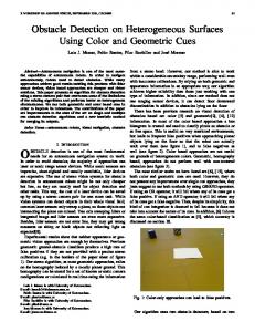
Fig. 1 –. Visualisation of the scenario

scenario, we affect their relative speed from the vehicle fitted with Laser and the way they run at start : on right or left. Then we set the parameters for the sensor. For example, the parameters we’ve worked with are : – the laser scanner is mounted at the left front of the car – it range from 0 to 270◦ in angle with 0.1◦ resolution – working distance is between 0 to 100 m – maximum laser reliability = 0.9 – the full scan in a way is made within 25 ms Then, an algorithm make the vehicles running, braking or doubling depending on safety distance at each sample time. The vehicles are reduced to a single point and we have position of the cars given by the scenario then we compute the angle and the distance for each one to the Laser knowing their position. Finally, a white gaussian noise is added to data before starting the fusion process.

2.2

Data fusion and tracking

We begin with the fusion between angle and distance using the Dempster-Shafer theory [5] and we continue with the algorithm proposed by M.Rombaut [6]. This algorithm make an association of the perceived vehicles with those which were known at the previous sample. So we test each couple (perceived, known) by computing a belief mass of relation between the two objects with Dempster-Shafer theory again. As only one perceived can be in relation with one known, we take the couple that have the higher belief. If a perceived is not in relation with another object that mean it may be a new object and if a known has no relation that mean the object may have disappear : either mask by another vehicle or out of range. When all cars are out of range, the simulation stops and an animated window showing the simulation is launched (Figure 1). In this window, we can see each vehicles perceived or not, the known one and the maximum of belief for couple that are supposed to be in relation. In the next section we introduce some concepts on the evidence theory.

3 3.1

Dempster-Shafer theory Concepts

Let Θ (which is referred to as the frame of discernment, or simple frame) be a set of mutually exclusive and exhaustive hypotheses about some problem domain (for simplicity, Θ will always

be assumed to be finite). Relevant propositions are presented as the subsets of Θ. The DempsterShafer theory started with the idea of using a number in the interval [0,1] to indicate the degree of evidence supporting a proposition. Specifically, based on observing evidence E, the function m(.) provides the following basic belief assignments (BBAs) on Θ : X

m : 2Θ → [0,1]m(∅) = 0

m(A) = 1.

(1)

A⊆Θ

The subset A of frame Θ is called the focus element of E, if m(A) > 0. Obviously, one difference between the theory of evidence and the Bayesian probability theory is that the Dempster-Shafer theory can directly assign a probability mass value to any subset of Θ, while Bayesian theory is restricted to only one of its elements. The belief measure and the plausibility measure of a proposition (represented by set B) are, respectively, defined as follows : bel(B) =

X

m(A)

(2)

A⊆B

X

pls(B) =

m(A)

(3)

A∩B6=∅

where bel(B) and pls(B) represent the lower bound and upper bound of belief in B. Hence, interval [bel(B),pls(B)] is the range of belief in B. If m1 and m2 are two BBAs induced from two independent evidence sources, and the condition X

ml (Ai )m2 (Bj ) < 1

(4)

Ai ∩Bj =∅

is met, then the combined BBA can be calculated according to Dempster’s rule of combination : m(C) = m1 (C) ⊕ m2 (C) = K ·

P Ai ∩Bj =C

m1 (Ai )m2 (Bj ),

m(C) = 0,

C 6= ∅ C=∅

where K represents the conflict between the two sources and is equal to : K=

1−

P Ai ∩Bj =∅

1 m1 (Ai )m2 (Bj )

(5)

Compared with the classical probability theory, the Dempster-Shafer theory has some attractive advantages, and one of the most important advantages is its ability to express degree of ignorance. In the Dempster-Shafer theory, the commitment belief to a subset does not mean the remaining belief should be committed to its complement. Consequently, the Dempster-Shafer theory provides a framework within which disbelief can be distinguished from a lack of evidence for belief. The next step is to associate objects using M. Rombaut algorithm. This algorithm will be describe in the following section.

3.2

Car association

Let Xi (i = 1 : n) be the perceived cars and Yj (j = 1 : m) the known one, we can define Θ with only two hypotheses : Θij = {Xi RYj ,Xi RYj } (6) Where (Xi RYj ) means that the perceived object Xi is in relation with the known object Yj whereas (Xi RYj ) means that a perceived object Xi is not in relation with the known one Yj .

The laser give us angle and distance for each perceived car, thus we can compute a belief mass for each hypotheses in case of angle and distance : mangle (Xi RYj ) = α0 · exp−ai,j i,j angle mi,j (Xi RYj ) = α0 · (1 − exp−ai,j ) mangle (Θi,j ) = mdistance (Θi,j ) = 1 − α0 i,j i,j

mdistance (Xi RYj ) = α0 · exp−di,j i,j distance mi,j (Xi RYj ) = α0 · (1 − exp−di,j )

where α0 is the reliability of the laser, ai,j is the mahalanobis distance between angles of car Xi and Yj and di,j is the mahalanobis distance between the distances of car Xi and Yj . Then, we fusion the two set of masses. The next step of M. Rombaut algorithm is to compute mi,. and the m.,j which correspond to mass fusion of the relation with a given object i and the j known objects and conversely : mi,. (Xi RYj ) = Ki,. · mi,j (Xi RYj ) · mi,. (Xi R∗) = Ki,. · mi,. (Θi,j ) = Ki,. · (

Q

(

Q

k=1:m,k6=j

(1 − mi,k (Xi RYk ))

(mi,j (Xi RYj ))

j=1:m

Q

(mi,j (Θi,j ) + mi,j (Xi RYj )) −

j=1:m

Ki,. =

Q

1

(1−mi,j (Xi RYj )))·(1+

j=1:m

m P

m

Q

(mi,j (Xi RYj )))

j=1:m

(Xi RYj ) )) i,j (Xi RYj )

i,j ( 1−m

j=1

Hypotheses (Xi R∗) is that the object Xi perceived is not in relation with any Yj . The m.,j are computed in analogy with mi,. . i,. and M .,j , and now we can choose the best Finally, we report the results in two matrix : Mcr cr couple according to the maximum of belief in the two matrix. Example with two objects known and two objects perceived, and we obtain the following matrices :

i,. Mcr

Y1 = Y2 ∗ Θi,j

X1 0.6 0.2 0.05 0.15

X2 0.3 0.5 0.15 0.05

.,j Mcr

= Y1 Y2

X1 0.6 0.4

X2 0.2 0.5

∗ 0.1 0.05

Θi,j 0.1 0.05

We can deduce from the first matrix that (X1 RY1 ) and (X2 RY2 ) (maximum of belief), and from the second one (X1 RY1 ) and (X2 RY2 ), so X1 is in relation with Y1 and X2 with Y2 is the best decision. The next section shows some results for a given scenario with the described method.

4

Results

Here are the result obtain for a scenario with 3 cars. The first car have a relative speed of 15 km/h and started on the right without offset time, the second one have a relative speed of 10 km/h and started on the right with an offset time of 5 s and the third one have a relative speed of 12 km/h and started on the left without offset time. Figure 1 shows a screenshot of this scenario at a given position/time. The advantage of a simulator is also that we can plot belief evolution for some varying parameters. We have plot for the vehicle 0 the belief with random loss of data (Figure 2), with the laser reliability a decreasing fonction of the distance (Figure 3), and both loss of data and varying reliability (Figure 4). The belief plotted in area 1 and 4 is (X0 R∗) : the car is not in the laser range and consequently not seen. In area 2 and 3, we have the belief of (X0 RY0 ) : the car is detected and followed. In

Fig. 2 –. Belief evolution of vehicle 0 taking into account loss of data

Fig. 3 –. Belief for vehicle 0 with a decreasing reliability

area 2 we can see that there are some points, around 1, detaching from the curve, it’s because the vehicle 0 is behind the vehicle 2 which is running less fast. The vehicle 0 brakes when the safety distance is too short, it relative speed is almost 0 and the detection by the laser is better. In area 3, the vehicle is running at the right at its constant speed. For the Figure 2, the belief is quite constant and close to 1. It’s because the laser reliability is set to 0.9, we just loose the vehicle (detaching points of the curve) when the sensor does not send any data. In case of Figure 3, the vehicle is always detected but the belief rise and fall because of the reliability rising when the vehicle approaches the sensor and decreasing when it run away. And the last case plotted on Figure 4, which best suits the reality, we combine both the loss of data and a varying reliability. As you can see, the belief is never under 0.585 with only one sensor. Furthermore, this minimum value is only due to the laser reliability : this minimum correspond to which appears in the Figure 3.

5

Conclusion

In this article, we have described a simulator which can let us evaluate some fusion algorithms for detection and tracking. The simulator let us use as much as sensors as we decide, we can also let the it run during the time we want, modify parameters like noise or loss of data and watch their impact on the algorithm, and we can create scenarios that normally append very few in real situations. The algorithm we have used was based on the evidence theory. Thanks to this algorithm, we can detect and follow some objects in a scene and we can set some varying parameters like sensor reliability. The simulator will be improved in those way : raise the number of sensor, varie the type of

Fig. 4 –. Vehicle 0 belief combining both loss of data and varying reliability

sensors, predict the position of cars with a Kalman filter and consider the car as a group of points.

Références [1] M. Bertozzi, A. Broggi, and A. Fascioli. Vision-based intelligent vehicles : state of the art and perspectives. Elsevier Robotics and Autonomus Systems, 32(1):1–16, June 2000. [2] D. Gruyer, C. Royère, R. Labayrade, and D. Aubert. Credibilistic multi sensor fusion for real time application. application to obstacle detection and tracking. IEEE International Conference on Advanced Robotics, ICAR’2003, University of Coimbra, Portugal, Juin 2003. [3] B. Dryselins, J. Broughton, L. Ekman, C. Hyden, G. Malaterre, S. Petica, R. Risser, and P. Van El Slande. Traffic safety in prometheus. Avril 1994. [4] A. Broggi, M. Bertozzi, A. Fascioli, C.G.L. Bianco, and A. Piazzi. Visual perception of obstacles and vehicles for platooning. IEEE Trans. on Intelligent Transportation Systems, 1(3):164–176, September 2000. [5] G. Shafer. A Mathematical Theory of Evidence. Princeton University Press, Princeton, New Jersey, 1976. [6] M. Rombaut. Decision in multi-obstacle matching process using the theory of belief. In AVCS’98, pages 63–68, 1998.