SIMULTANEOUS SCHEDULING OF MACHINES AND OPERATORS ...

SIMULTANEOUS SCHEDULING OF MACHINES AND OPERATORS IN A MULTIRESOURCE COINSTRAINED JOB-SHOP SCENARIO Lorenzo Tiacci(a), Stefano Saetta(b) (a) (b)

Dipartimento di Ingegneria Industriale – Università degli Studi di Perugia Via Duranti, 67 – 06125 Perugia - Italy (a)

[email protected], (b)[email protected]

ABSTRACT In the paper the simultaneous scheduling of different types of resources is considered. The scenario is constrained by machines and human resources, and its complexity is increased by the presence of two types of human resources, namely the equipper, that performs only an initial action of each task (the ‘setup’), and the normal operator, that loads and unloads each piece from machines. A conceptual model of the shop is build in order to simultaneously handle priority rules for each one of the three types of resources considered (machine, equipper and operator). A simulation model has been implemented and a simulation experiment performed in order to explore the effect on mean flow factor reduction of different combination of priority rules. Keywords: dual-resource constraints, multi-resource constraints, priority rule scheduling, job shop control.

1.

INTRODUCTION

Job shop scheduling has attracted researchers for many decades, and still now is one of the most studied subjects in literature related to industrial problems. However, multi or dual resource constrained scheduling problems are significantly less analyzed, although being more realistic (Scholz-Reiter, Heger and Hildebrandt 2009). ElMaraghy, Patel and Abdallah (2000) defined the machine/worker/job scheduling problem as: “Given process plans for each part, a shop capacity constrained by machines and workers, where the number of workers is less than the number of machines in the system, and workers are capable of operating more than one machine, the objective is to find a feasible schedule for a set of job orders such that a given performance criteria is optimized”. Optimal solution are difficult to find also for the single resource scheduling problem, so that many heuristics approaches have been used in literature to find good but non optimal solutions for the machine constrained problem. These approaches include: Simulating annealing (Laarhoven, Aarts and Lenstra 1992); Genetic algorithms (Zhou, Cheung and Leung

2009; Manikas and Chang 2008); Tabu search (Zhang, Li, Guan and Rao 2007)). Complexity increases in dual resource constrained problems, and extending these often quite complex heuristics to more realistic scenarios is usually not straightforward. Dauzère-Pérès, Roux and Lasserre (1998) developed a disjunctive graph representation of the multi-resource problem and proposed a connected neighborhood structure, which can be used to apply a local search algorithm such as tabu search. Matie and Xie (2008) developed a greedy heuristic guided by a genetic algorithm for the multi-resource constrained problem. However, in most real-world environments, scheduling is an ongoing reactive process where the presence of a variety of unexpected disruptions is usually inevitable and continually forces reconsideration and/or revision of pre-established schedules (Ouelhadj and Petrovic 2009). Most of the above-mentioned approaches have been developed to solve the problem of static scheduling and are often impractical in real-world environments, because the near-optimal schedules with respect to the estimated data may become obsolete when they are released to the shop floor. As a result, Cowling and Johansson (2002) addressed an important gap between scheduling theory and practice, and stated that scheduling models and algorithms are unable to make use of real-time information. A quick, intuitive, and easy to be implemented method for dynamic scheduling is utilizing priority (or dispatching) rules. The application of priority rules gives raise to a completely reactive scheduling, where no firm schedule is generated in advance and decisions are made locally in real-time. A priority rule is used to select the next job with highest priority to be assigned to a resource. This is done each time the resource gets idle and there are jobs waiting. The priority of a job is determined based on job, machine or in general resources attributes. Priority-scheduling rules have been developed and analyzed for many years (Haupt 1989, Blackstone, Philips and Hogg 1982, Rajendran and Holthaus 1999, Geiger, Uzsoy and Aytu 2006, Geiger and Uzsoy, 2006). Although priority rules have also been applied to

dual-resource constrained problems (Scholz-Reiter, Heger and Hildebrandt, 2009), there are no studies in literature that deal with the presence of different types of human resources, each one competent to perform a specific action of the job cycle. In fact, resources heterogeneity is usually considered just in terms of different work efficiency of resources on different tasks. In this work we analyze a multi-resource constrained job-shop scenario in which scheduling is constrained by machines and by two types of human resources, namely ‘equippers’ and ‘operators’. Equippers and operators do not perform the same action with different efficiency, but are assigned to completely different and non-overlapping actions related to the job cycle. A conceptual model of the company’s shops is built in order to simultaneously handle priority rules for each one of the three types of resources considered (machine, equipper and operator). A simulation model has been built and a simulation experiment performed in order to explore the efficacy on flow factor reduction of different combination of priority rules. The paper is organized as follows. The job shop scenario is described in section 2. In section 3 the conceptual model of the shops is illustrated. Section 4 deals with the implementation of the simulation model, while in section 5 the simulation experiment is described and results are discussed. In section 6 conclusions are drawn. 2.

THE JOB-SHOP SCENARIO

The scenario is representative of a real case study of a manufacturing company in the field of precision metal and mechanical processing. The company is specialized in the production of very complex components for industrial, aeronautical and aerospace applications. In the aerospace and aeronautical fields, the company produces 1/A class components such as, for example, actuators, stabilizers, worm gears, landing devices, turbine’s bearing rings and axle rotors. In the industrial sector, the company produces high quality components for machine tools and laser cutting. 2.1. Areas The company is organized in different areas, in which there are homogeneous machines. Every job assigned to a certain area can be processed indifferently in one of the machine belonging to that area. There are 5 areas: the cutting area, area 1 (turning), area 2 (milling), area 3 (drilling), and a control area. The cutting area and the control area are not critic for the scheduling problem, because resources assigned to these areas do not constrain the solution. However, they have been considered in our model in order to get a realistic representation of the flow time of each job. 2.2. Jobs Each job is represented by (see Fig. 1): 

a quantity of pieces that have to be processed (lot size);

  

a set of tasks that have to be performed on each piece of the job, and the associated area; the sequence of tasks that have to be performed; the processing times of actions connected to each task.   Task  sequence  Task  1  Turning                     2  Turning                     3  Milling                      4  Milling                      5  Control

  

     

JOB 1 (lot size: 9)  AREA  AREA 1  ACTION  TIME (min)  Set‐up  0.85 Load  2.5 Run  5 Unload  2.5 Inspection  5 AREA 1  ACTION  TIME (min)  Set‐up  131.45 Load  2.5 Run  3 Unload  2.5 Inspection  5 AREA 2  ACTION  TIME (min)  Set‐up  203.92 Load  2.5 Run  45 Unload  2.5 Inspection  5 AREA 2  ACTION  TIME (min)  Set‐up  202.93 Load  2.5 Run  45 Unload  2.5 Inspection  5 CONTROL AREA     ACTION  TIME (min)  Control   15

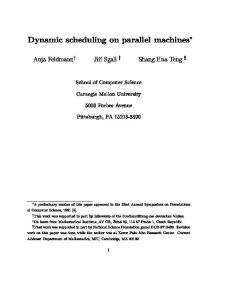
Figure 1: Example of data representing a job. 2.3. Machines In each area of interest (areas 1,2 and 3) there are computer numerical control (CNC) machines. Each machine can be equipped with a variable set of tools that allow completing the run with no interruptions. Every time a job is changed, the set of tools have to be changed depending on the new task requirements, and the controlling software has to be appropriately programmed. Then each piece belonging to the job has to be loaded, processed (run), and unloaded. After the first piece of a job has finished its run and has been unloaded, it must be inspected before that the remaining pieces of the lot can start being processed (see Figure 2). 2.4. Equippers The machine set-up is performed by the equipper operator at the beginning of each task, before processing the first piece of the lot. The inspection action on the first piece is also performed by the equipper, that controls if the run has been properly executed. If everything is ok, the other pieces of the lot can start to be processed, and load and unload operations are then carried out by the normal operator,

without the need of the participation of the equipper. The equippers assigned to a certain area are able to equip all the machines inside that area. 2.5. Operators The normal operator performs loading and unloading of the pieces of a job. Processing starts directly after the machines are loaded. Unloading begins after processing, but if there is no operator available for unloading, the machine stays idle. The operators are not needed during processing and can work on other machines in that time period. The operators assigned to a certain area are able to load/unload all the machines inside that area.

Equipper Operator Machine the job starts setup

setup Load

1st piece

Load

run

unload inspection

unload inspection

Load

2nd piece

Load

time

run

unload

unload

Load

Load

3nd piece

3.

run

unload

unload

…

…

Figure 2: Actions involving the different resource types. 2.6. Shifts An important feature of the scenario is that shifts are different between Equippers and Operators. The operators work is organized in three shifts per day, each shift during 8 hours. Equippers work on a single shift per day, from 8.00 to 17.00, with an interval of one hour between 13.00 and 14.00. Thus, while operators (as machines) are available during all the 24 hours, equippers are available only in the central part of the day. The number of resources per shift in each area is reported in Table 1. Table 1: Resources Availability

Machines 24h/day

Area 1 Area 2 Area 3

4 4 3

Equippers 8.00-13.00 14.00-17.00 2 1 2

2.7. The company’s scheduling process Production scheduling is performed through a commercial software that considers different types of resources, such as machines, operators, equipments, transporters etc. However, the scheduling is done primarily only considering the machines as limiting resource. Then, the resulting schedule is verified, checking if the capacity constraints related to the other resources are respected. In case of capacity shortages, the solution can be manually modified, for example by introducing overtime, or re-calculated, by modifying jobs due dates. This approach however does not allow a real simultaneous scheduling of machines and human resources, and the ‘trial and error’ nature of the procedure make it quite rigid, and unsuited to reacting to uncertainties of the environment. Furthermore, in the specific case study, the equipper (the most specialized human resource) is not always available during the day (see Table 1) and this makes it the primary candidate for being the limiting resource in many situations. In the next paragraphs, we describe an alternative way to approach the scheduling problem, based on dispatching rules. The approach developed is based on the fact that, besides the rules considered to assign jobs to machines, it is necessary to simultaneously consider the rules to assign operators and equippers to jobs.

Operators 24h/day 3 1 2

THE CONCEPTUAL MODEL

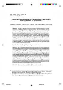
The systems has been modeled through a series of queues, some of which are ordered following different possible priority rules, through which decide the pickup order of the elements. The logical flow of entities in the systems is depicted in Fig. 3 (where AREA 2 is considered). There are 4 types of queues in each area, namely: PQ1, PQ2, VQ1 and VQ2. When a new job arrives, it tries to enter the area corresponding to the task that has to be performed. If all the machines in that area are busy, the job has to wait in a queue of type PQ1. When one of the machines in the area is free, the job is assigned to that machine, and the lot is divided into a number of pieces equal to the lot size. Pieces are then allocated in the PQ2 queue of the assigned machine (input buffer). Pieces in PQ2 queues may claim an equipper or an operator, depending on the action needed to complete their current task. If they claim an equipper, they also enter the virtual queue VQ1, which is served from the equippers of the area; if they claim an operator, they also enter the VQ2, which is served from the operators of the area. When an equipper or an operator is available, pieces are removed from VQ1 or VQ2, and the required action on the pieces are performed. When a task of a job has been completed, i.e. the last piece of the lot has been unloaded from the machine, the machine is released, and the job tries to enter the area corresponding to the next task of its processing sequence.

Considering each area, we classify the queues into physical and virtual queues.

Note that while rules 1 to 5 are related to a local characteristic of the queue, rules LMQL and SMQL are taken on the basis of the length of PQ2 queues.

3.1. Pysical Queues (PQ)  PQ1. The first physical queue is related to jobs that are waiting for entering an area. The queue is physical because we can associate a job to the lot that is waiting (in a trolley for example) in a certain part of the shop. Jobs are picked up from this queue as soon as one of the machines of the area is available to work. Each area has one queue of type PQ1.  PQ2. The second physical queue is related to pieces of jobs that are waiting to be processed by a machine, i.e. they belong to a job that has already been assigned to a machine, and are waiting in the input buffer of the machine. Each machine has one queue of type PQ2.

AREA 2 P

M P

3.3. Priority rules Priority rules are defined to select elements waiting in PQ1, VQ1 and VQ2 queues. These queues are the ones to which priority rules are applied, because elements of these queues claim a resource: PQ1 - machines, VQ1 equippers and VQ2 - operators. The priority rules for PQ1 (machines) are: 1. FIFO (First-IN, First-OUT); 2. LIFO (Last-IN, First-OUT); 3. SPT (Shortest Processing Time); 4. LPT (Longest Processing Time); 5. RANDOM; In addiction to these 5 rules, we considered two additional decision rules for VQ1 (equippers) and VQ2 (operators): 6. LMQL (Longest Machine Queue Length); 7. SMQL (Shortest Machine Queue Length).

P

P

P

P

P

PQ2

M P

P

P

P

PQ2 J

J

J

M

PQ1

3.2. Virtual queues (VQ)  VQ1. The first virtual queue is related to pieces of jobs that are waiting for an equipper, i.e., the first pieces of a job that have been already assigned to an available machine and are waiting or for the setup action on the machine, or for the inspection action. Each area has one queue of type VQ1.  VQ2. The second virtual queue is related to pieces of jobs that are waiting for an operator, i.e., pieces belonging to jobs already initiated, and waiting for loading or unloading actions. Each area has one queue of type VQ1. It is noteworthy that VQ1 and VQ2 are not physical queues. In particular, elements waiting in VQ1 can be physically in the input buffer of a machine (the first piece of a job waiting for the setup action) or in the machine itself (the first piece of a job waiting for the inspection action). Similarly, elements waiting in VQ2 can be physically in the input buffer of a machine (waiting for load action) or inside the machines (waiting for unload action).

E

P

VQ1

P

P

P

P

P

P

PQ2

M P

P

P

P

PQ2

P

P

O

VQ2

Figure 3: Queues and logical flow (J = job; P = piece)

4.

THE SIMULATION MODEL

The simulation model has been built with Arena 11, using basic process, advanced process, advanced transfer, calendar schedules, and animation tools. In the next section, the main part of the model implementation is described. 4.1. The simulation model implementation The basic entity is one piece of a job. Pieces are batched, and batches move through the system when they move between different areas. A batch is separated into pieces when the job enters an area and pieces have to be processed in the machines. Machines, Operators and Equippers are modeled as Resources. The number of operators and equippers in each shift (see Table 1) is modeled using the Calendar Schedule utility of Arena, through which the detailed time patterns and the capacity of each resource can be set up.

Creation

Attributes

Read job data

Batch

0 0

Figure 4: Pieces and job creation

A piece is created and a series of attributes are assigned to it (e.g. the job code, the current time). Then other attributes related to the job (lot size, tasks, actions times, tasks sequence etc.) are read from file. Pieces are batched according to the lot size of the job, and the batch proceeds to the area of destination, according to its task sequence. The Route and Station modules of the Advanced Transfer tools of Arena have been utilized to perform entities movements throughout the model. The system is modeled through different sets of Station: Area Stations, Machine Stations, Equipper and Operator Stations, Actions Stations. 4.1.1. Area Stations An Area Station is associated to each area of the shop floor. When a batch arrives at the Area Station (e.g. Area 3 in Figure 5), it enters PQ1 queue of the area. The order of the queue can be set according to one of the priority rules (1-5) defined in section 3.3. A batch can leave the queue according to a ‘scan for condition’ rule. The condition is verified when at least one of the PQ2 queues of the machines in the area is empty. The decide module directs the batch to the Station related to the available machine. GO TO MACHINE M1

GO TO MACHINE M2

AREA 3

PQ1 AREA 3

Decide GO TO MACHINE M3 E lse

Dispose

Figure 5: Area Stations. 4.1.2. Machine Stations A Machine Station is associated to each machine of an area. When the batch arrives to the machine (e.g. machine M1 in Figure 6), it is separated into pieces. A Counter module and a Decide module allow to identify the first piece of the job (the related attribute ‘First Piece’ is associated to the entity). An attribute (named ‘Current Machine’), related to the machine to which the piece has been assigned, is also stored. Then the entity moves to the Seize module corresponding to the PQ2 queue of the machine. The seize module is associated to a virtual resource of fixed capacity equal to 1, that is seized when the entity exits the queue, and is released by the same entity when all the actions associated to its task on the machine have been performed (see later in section 4.1.4). The introduction of this virtual resource is necessary because when the entity exits the queue and seizes the resource, this means that one machine is available to work, but not that the machine will be immediately seized: in fact, the piece could have to be waiting for an equipper or an operator to be loaded in or unloaded from the machine. So, the seize module cannot be associated to the machine resource if one want to accurately evaluate the actual machine utilization.

0 MACHINE M1

Separate

0

True

First Piece?

0

Counter

Assign First Piece of the Job Attribute

Assign Machine M1

False

0 PQ2 M1

Assign number of pieces in PQ2 M1

First Piece

0

True

GO T O EQUIPPER

False

RESET COUNTER

GO T O OPERAT OR

Figure 6: Machine Stations. When a piece exits the PQ2 queue, an attribute describing the length of that queue is assigned. This will allow ordering the succeeding VQ1 or VQ2 queues on the basis of this attribute, in order to implement rules 6 and 7. After that, another Decide module sends the entity to the Equipper or the Operator Station modules, depending on the ‘First Piece’ attribute. 4.1.3. Equipper and Operator Stations There are one Equipper Station and one Operator Station for each area of the shop floor. When a piece arrives to the Equipper Station of an area (Figure 7) it enters the Seize module corresponding to the VQ1 queue of the area. The order of the queue can be set according to one of the priority rules 1-7. The Seize module is associated to the Equipper resource of the area, whose capacity is set up through the Calendar Schedule utility. If at least one equipper is available, the piece exits the queue and seizes the equipper, which will be then released by the same entity when the action performed by the equipper (set up or inspection) has been performed. The Decide module directs the entity to the Station corresponding to the next action to be performed on the machine. This is possible thanks to the ‘current machine’ attribute (previously assigned to the entity), and another entity attribute, which is updated during the model execution, that describes the next action that the entity has to perform. GO TO SETUP M1

GO TO SETUP M2

EQUIPPER Station

VQ1 Area 3

GO TO SET UP M3

Action and Machine?

E lse

USO USO USO USO USO USO

M1==100& & C ON TR OLLO==0 M2==100& & C ON TR OLLO==0 M3==100& & C ON TR OLLO==0 M1==100& & C ON TR OLLO==100 M2==100& & C ON TR OLLO==100 M3==100& & C ON TR OLLO==100

GO TO INSPECTION M1

GO TO INSPECTION M2 Dispose 7

0

GO TO INSPECTION M3

Figure 7: Equipper Stations. If the piece is directed to the Operator Station (Figure 8), it follows a very similar path. Here the queue is the VQ2 queue, which can be ordered according to

priority rules 1-7. The associated resource that will be seized is one operator of the area. GO TO LOAD M1

GO TO LOAD M2

GO TO LOAD M3 OPERATOR Station

Decide 5

VQ2 AREA 3

GO TO UNLOAD M1 Else

GO TO UNLOAD M2

GO TO UNLOAD M3

Dispose 9

0

Figure 8: Operator Stations. 4.1.4. Action Stations There are four Action Stations for each machine. Each station is related to a determined action performed by equippers or operators on the machine, namely: set up, load, unload and inspection (see Figure 9). A piece that arrives at the setup Station is necessarily coming from the equipper Station (Figure 7), where it had seized one equipper. The entity now seizes the machine, and is delayed by a time equal to the setup time. Then it releases the equipper (but not the machine) and is routed toward the Operator Station. A piece that arrives at the load Station it is necessarily coming from the Operator Station (Figure 8), where it had seized one operator. If the piece is the first one of the job, the machine must not be seized, because it has already been seized during the setup. The entity is here delayed for an amount of time equal to the load action, after which releases the operator (but not the machine). The succeeding delay module corresponds to the run action performed by the machine. An attribute specifying the next action to be performed (unload) is stored before the entity is routed again towards the Operator Station. SET UP M1

Seize M1

0 LOAD M1

First Job?

0

GO TO OPERATOR Station

Release EQUIPPER M1

Delay SETUP M1

T ru e

Delay LOAD M1

Release OPERATOR M1

Delay RUN M1

next action UNLOA D

GO TO OPERATOR Station

Fa ls e

Seize M 1

UNLOAD M1

Delay UNLOAD M1

Release OPERATOR M 1

0 First job?

0

INSPECTION M1

Delay INSPECTION M1

Release EQUIPPER M 1

T ru e

GO TO EQUIPPER Station

next action INS P E CTION

Fals e

Release M1

Release PQ1 M1

next area and next action

B atch pieces

GO TO NEXT AREA Station

0

Figure 9: Actions Stations When a piece arrives to the unload Station (coming from an Operator Station, where it had seized an operator), it is delayed for unloading, and then it releases the operator. If the piece is the first of the job, it has to be inspected by an equipper: the opportune next action attribute (inspection) is stored, and the entity is routed towards the Equipper Station. Otherwise the piece has finished his task in the machine: it releases the machine and then releases the virtual resource

associated to the PQ1 queue of the machine (to allow a new piece to be loaded by an equipper or an operator, see Figure 6). The opportune ‘next action’ and ‘next area’ attributes are stored, and finally the piece enters the batch module. A similar path is followed by the first piece of a job that arrives to the inspection Station. The only difference is that the entity is delayed for a time equal to the inspection time, and then releases the equipper. When all the pieces of the job have been processed, the batch is ready to be routed to the next area of destination. 4.2. Verification and validation During the time for the simulation model realization, many meetings with company’s managers have been organized. For the valid modelisation of the human resources (operators and equippers) and the possible scheduling logic that could be implemented, the continuous confrontation with company’s staff during the model development has been very profitable. In this way, the essential aspects of the scheduling and the production processes have been outlined by those which operate in the day by day operations activities in the company. This confrontation also brought to renounce adopting complicated approach that are often studied by a theoretical point of view, but that are scarcely applicable to real cases. This allowed also to gain the company’s management accreditation for the use of simulation for the specific purpose of searching for alternative scheduling techniques with the aim to reduce the jobs mean flow factor. The conceptual model has been validated by the operational experts of the company: they confirmed that the assumptions underlying the proposed conceptual model were correct and that the proposed simulation design elements and structure (simulation’s functions, their interactions, and outputs) would have lead to results realistic enough to meet the requirements of the application. After the implementation, the same experts, comparing the responses of the simulation with expected behaviours of the system, confirmed that those responses were sufficiently accurate for the range of intended uses of the simulation. We also verified our model through two widely adopted techniques (see Law and Kelton, 2000). The first one consists in computing exactly, when it is possible and for some combination of the input parameters, some measures of outputs, and using it for comparison. The second one, that is an extension of the first one, is to run the model under simplifying assumptions for which its true characteristics are known and, again, can easily be computed. Furthemore, in order to check the correct implementation of dispatching rules logic, the animation capability of Arena has also been exploited (see Figure 10).

Heger and Hildebrandkt, 2009) or ‘Stretch’ (Bender, Muthukrishnan and Rajaraman, 2004) to measure the effect of scheduling on an individual job. The Flow Factor (or Stretch) of a job is the ratio of its Flow Time to its Processing Time: [C(i) - r(i)]/p(i). Flow factor is particularly suited in this case, where multiple jobs with different processing times are considered. The mean flow factor of all the jobs has been indicated by the expert personnel of the company as the measure through which compare different scheduling combinations of dispatching rules. In particular, each combination can be compared also with the scheduling decided by the company in the same period, that obtained a mean flow factor equal to C = 27.33.

Figure 10: A screenshot of the animation. 5.

5.2. Results Figure 11 shows the simulation experiment results related to the first part (same equippers and operators rules).

THE SIMULATION EXPERIMENT Table 2: The simulation experiment results (first part).

The simulation experiment is conducted using real data provided by the company, and refers to orders arrived during 4 months, for a total number of different jobs equal to 24. Processing times performed by equippers and operators have been modeled as normal distributed. Standard deviations data were available for some of the considered jobs, those ones that had already been manufactured by the company and for which worksampling activities had already been performed. A coefficient of variation equal to 0.03 has been assumed for new jobs, accordingly to historical data related to similar jobs. The simulation experiment is divided into two parts. In the first one it is assumed that the same decision rule is assigned both to equippers and to operators. So different scenarios have been evaluated considering all the 5x7 = 35 combinations of the 5 decisions rules for machines (queue PQ1) and the 7 decision rules for operators and equippers (queues VQ1 and VQ2). The aim is to find the best rule for machines, and then to perform the second experiment maintaining the selected machines rule fixed, and exploring all the 7x7 combinations of rules for equippers and operators. This is performed in the second part of the experiment. Each scenario has been replicated 20 times. 5.1. Performance Measures Traditionally, the focus of performance in this type of scheduling problems has been on the Flow Time, which is defined as the amount of time that a given job spends in the system. If the i-th job arrives at time r(i), has Processing Time p(i) (that is known at the time of its arrival), and a Completion Time C(i), its flow time will be C(i) - r(i). However, Flow Time measures the time that a job is in the system regardless of the service it requests. Relying on the intuition that a job that requires a long service time must be prepared to wait longer than jobs that require small service times, practitioners and researchers have used the ‘Flow Factor’ (Scholtz-Reiter,

equippers and operators rule (VQ1 and VQ2)

MEAN FLOW FACTOR

P-Value

FIFO

FIFO

30.14

1.000

FIFO

LIFO

29.54

1.000

FIFO

LMQL

32.42

1.000

FIFO

LPT

32.01

1.000

FIFO

RND

34.49

1.000

FIFO

SMQL

28.38

1.000

FIFO

SPT

28.92

1.000

LIFO

FIFO

32.39

1.000

LIFO

LIFO

32.84

1.000

LIFO

LMQL

38.04

1.000

LIFO

LPT

31.88

1.000

LIFO

RND

32.76

1.000

LIFO

SMQL

28.94

1.000

LIFO

SPT

29.55

1.000

LPT

FIFO

37.40

1.000

LPT

LIFO

35.63

1.000

LPT

LMQL

41.05

1.000

LPT

LPT

40.09

1.000

LPT

RND

37.65

1.000

LPT

SMQL

35.41

1.000

LPT

SPT

36.67

1.000

RND

FIFO

26.27

0.369

RND

LIFO

25.74

0.001

RND

LMQL

29.43

1.000

RND

LPT

28.42

1.000

RND

RND

26.22

0.278

RND

SMQL

28.21

1.000

RND

SPT

25.12

0.000

SPT

FIFO

24.39

0.000

SPT

LIFO

24.17

0.000

SPT

LMQL

26.16

0.170

SPT

LPT

25.94

0.018

SPT

RND

25.85

0.006

SPT

SMQL

22.77

0.000

SPT

SPT

22.00

0.000

machine rule (PQ1)

processing time jobs at the end of the shift. In this way there is a higher probability that jobs starting at the end of the shift will last a reasonable amount of time, and that the successive set-up will not occur just a short time after the end of the equipper shift.

Main Effects Plot (data means) for MEAN FLOW FACTOR machine rule (PQ1)

equip. & oper. rules (VQ1 & 2)

Mean of MEAN FLOW FACTOR

37.5 35.0

Table 3. Main effects for Mean Flow Factor.

32.5 30.0

equippers rule (VQ1)

27.5

25.0 FIFO

LIFO

LPT

RND

SPT

FIFO

LIFO LMQL

LPT

RND SMQL

SPT

Figure 11. Main effects for Mean Flow Factor, first experiment. The table reports the average value  (over 20 replications) of the Mean Flow Factor for each scenario. The P-Value of the t-test in the last column indicates the smallest level of significance at which the null hypothesis (H0:  = C) would be rejected in favor of the alternative hypothesis (H1:  < C). The lowest value of mean flow factor is obtained when the Short Processing Time (SPT) rule is adopted for all the resources of the system (machines, operators and equippers). It is noteworthy that in the most part of scenarios obtaining a mean flow factor significantly lower than the one obtained by the company, the SPT rule is adopted for machines. Figure 11 reports the main effects plots for Mean Flow Factor, in which is also shown that SPT is the machine rule that performs better in combination with all the other equippers and operator rules. In the second experiment the machines rule was fixed (SPT), while all the combination of equippers and operators rules have been evaluated. Results are reported in Table 3. It is easy to see that the number of scenarios with  < C is significantly higher. The best combination is obtained when also equippers follow the SPT rule, while operators follow the SMQL rule. Main effects plots (reported in Figure 12) confirm that these rules are the ones that on the average perform better when combined with all the other rules. Some considerations about the validity of these rules for equippers and operators can be drawn. Equippers are available only in the central part of the day (see Table 1), while machines and operators are available during all the 24 hours. An undesirable situation would be that a machine has to be set up when the equippers are not available (eg. during the night). This would cause in fact an idle time both for the machine and potentially for operators, that cannot proceed with load and unload actions on the pieces of the job. A good situation would be that the equipper set up the machine during its shift in such a way that machines and operators can continue processing the job during the night, without the need of a set-up. By giving precedence to jobs with the shortest processing time during its shift, the equipper tends to serve the longest

operators rule (VQ2)

MEAN FLOW FACTOR

P-Value

FIFO

FIFO

24.39

0.000

FIFO

LIFO

25.38

0.000

FIFO

LMQL

27.82

1.000

FIFO

LPT

25.19

0.000

FIFO

RND

24.47

0.000

FIFO

SMQL

23.47

0.000

FIFO

SPT

23.72

0.000

LIFO

FIFO

23.64

0.000

LIFO

LIFO

24.17

0.000

LIFO

LMQL

25.87

0.008

LIFO

LPT

25.85

0.006

LIFO

RND

0.085

LIFO

SMQL

26.08 21.78

LIFO

SPT

22.06

0.000

LMQL

FIFO

25.38

0.000

LMQL

LIFO

24.28

0.000

LMQL

LMQL

26.16

0.170

LMQL

LPT

24.59

0.000

LMQL

RND

24.91

0.000

LMQL

SMQL

23.28

0.000

LMQL

SPT

23.73

0.000

LPT

FIFO

25.79

0.003

LPT

LIFO

24.01

0.000

LPT

LMQL

27.34

1.000

LPT

LPT

25.94

0.018

LPT

RND

23.14

0.000

LPT

SMQL

24.79

0.000

LPT

SPT

25.31

0.000

RND

FIFO

25.58

0.000

RND

LIFO

23.67

0.000

RND

LMQL

28.44

1.000

RND

LPT

24.20

0.000

RND

RND

0.000

0.000

RND

SMQL

23.56 21.96

RND

SPT

22.77

0.000

SMQL

FIFO

24.64

0.000

SMQL

LIFO

25.33

0.000

SMQL

LMQL

24.65

0.000

SMQL

LPT

24.25

0.000

SMQL

RND

22.72

0.000

SMQL

SMQL

22.77

0.000

SMQL

SPT

22.59

0.000

SPT

FIFO

22.91

0.000

SPT

LIFO

23.79

0.000

SPT

LMQL

25.15

0.000

SPT

LPT

25.05

0.000

SPT

RND

0.000

SPT

SMQL

23.30 21.51

0.000

SPT

SPT

22.00

0.000

0.000

over performs the company’s scheduling. The approach allows to gain insights into priority rule performance, and to individuate a simple and implementable scheduling logic that provides a completely reactive scheduling.

Main Effects Plot (data means) for MEAN FLOW FACTOR equippers rule (VQ1)

Mean of MEAN FLOW FACTOR

27

operators rule (VQ2)

26

25

Aknolwedgments Authors thanks Dr. Cristiano Antinori for his supporting activity during the model implementation.

24

23 FIFO

LIFO LMQL

LPT

RND SMQL

SPT

FIFO

LIFO LMQL

LPT

RND SMQL

SPT

Figure 12. Main effects for Mean Flow Factor, second experiment. As far as the SMQL rule for the operators is concerned, it is noteworthy the importance to implement a rule that is not based on a job attribute, but on a machine attribute (PQ2 queue length). On the basis of the two preceding choices dictated by machine and equipper rules, the operator has only to choose among jobs that have already been assigned to a machine and set-up. In this case, serving the machine with the lowest number of pieces in the queue means to speed up the machine release, and to favor the entering of a new job. Possible improvements in the application of dispatching rules to this job shop scenario could be reached by allowing the selection of dispatching rules depending from time. For example, it would be possible to assign the SPT rule for the equipper in the first part of its shift and the LPT in the final part, in order to increase the probability that the successive set-up will not be needed just little time after the finish of the equipper shift. Analogously, dispatching rules for machines and operators could be differentiated in the case the equippers are present (the central shift of the day) with respect to when they are not.

6.

SUMMARY

In the paper a job-shop scheduling scenario is considered, derived from a case study of a manufacturing company that works for the aeronautical industry. A conceptual model of the shops has been built in order to implement a priority rules approach for the simultaneous scheduling of machines and two types of human resources: equippers and operators. The modelisation through virtual and physical queues allowed to define rules that are related both to jobs attributes and to machines attributes, and facilitated the implementation of a simulation model. Different combination of priority rules for machines, equippers and operators have been simulated and results have been compared on the basis of the mean flow factors of the considered jobs. Results have been compared to the mean flow factor obtained by the company for the same input data, and allow identifying the best rules combination that

REFERENCES Bender, M.A., Muthukrishnan, S., Rajaraman, R., 2004. Approximation algorithms for average stretch scheduling. Journal of Scheduling, 7, 195-222. Blackstone, J.H., Philips, D.T., Hogg, G.L., 1982. A state-of-the-art survey of dispatching rules for manufacturing job shop operations. International Journal of Production Research, 20(1), 27-45. Cowling, P. I., Johansson, M. (2002). Using real-time information for effective dynamic scheduling. European Journal of Operational Research, 139(2), 230–244. Dauzère-Pérès, S., Roux, W., Lasserre, J.B., 1998. Multi-resource shop scheduling with resource flexibility. European Journal of Operational Research, 107(2), 289-305. ElMaraghy, H., Patel, V., Abdallah, I.B., 2000. Scheduling of manufacturing systems under dualresource constraints using genetic algorithms. Journal of Manufacturing Systems, 19(3), 186201. Geiger, C., Uzsoy, R., Aytu, H., 2006. Rapid modeling and discovery of priority dispatching rules: an autonomous learning approach. Journal of Scheduling, 9, 7-34. Geiger, D., Uzsoy, R., 2006. Learning effective dispatching rules for batch processor scheduling. International Journal of Production Research, 46(6), 1413-1454. Haupt, R., 1989. A survey of priority rule-based scheduling. OR Spectrum, 11, 3-16. Laarhoven, P.J.M.v., Aarts, E.H.L., Lenstra, J.K., 1992. Job shop scheduling by simulated annealing. Operations Research, 40(1), 113-125. Manikas, A., Chang, Y., 2009. Multi-criteria sequencedependent job shop scheduling using genetic algorithms. Computers & Industrial Engineering, 59(1), 179-185. Matie, Y., Xie, X., 2008. A genetic-search-guided greedy algorithm for multi-resource shop scheduling with resource flexibility. IIE Transactions, 40(12), 1228-1240. Ouelhadj, D., Petrovic, S., 2009. A survey of dynamic scheduling in manufacturing systems. Journal of Scheduling, 12, 417-431. Rajendran, C., Holthaus, O., 1999. A comparative study of dispatching rules in dynamic flowshops and

jobshops. European Journal of Operational research, 116, 156-170. Scholz-Reiter, B., Heger, J., Hildebrandt, T., 2009. Analysis and comparison of dispatching rule-based scheduling in dual-resource constrainted shopfloor scenarios. Proceedings of the World Congress on Engineering and Computer Science, pp. 921-927. October 20-22, San Francisco (California, USA). Zhang, C., Li, P., Guan, Z., Rao, Y., 2007. A tabu search algorithm with a new neighborhood strucutre for the job shop schedulino problem. Computers & Operations Research, 34(11), 32293242. Zhou, H., Cheung, W., Leung, L.C., 2009. Minimizing wighted tardiness of job-shop scheduling using a hybrid genetic algorithm. European Journal of Operational Research, 194(3), 637-649.

AUTHORS BIOGRAPHY Lorenzo Tiacci. Laurea Degree in Mechanical Engineering, doctoral Degree in Industrial Engineering, he is Assistant Professor at the Department of Industrial Engineering of the University of Perugia. He is currently teaching courses of Facilities Planning & Design, Production Planning and Control, and Project Management at the University of Perugia. His research activity covers modeling and simulation of logistic and productive processes, plants design, production planning and inventory control, supply chain management, transportation problems. Stefano Saetta. Stefano SAETTA is Associate Professor at the Engineering Faculty of the University of Perugia. His research fields covers essentially the following subjects: modelling and simulation of logistic and productive processes, methods for the management of life cycle assessment, discrete event simulation, supporting decision methods, lean production. He was involved in several national and international research projects He is the organising committee and in the scientific committee of many international conferences.