Konrad-Zuse-Zentrum fur ¨ Informationstechnik Berlin
T OBIAS ACHTERBERG ¨ M ARTIN G R OTSCHEL T HORSTEN KOCH
Software for Teaching Modeling of Integer Programming Problems
ZIB-Report 06-23 (May 2006)
Takustraße 7 D-14195 Berlin-Dahlem Germany
Software for Teaching Modeling of Integer Programming Problems∗ Tobias Achterberg†
Martin Gr¨otschel†
Thorsten Koch†
June 1, 2006
Abstract Modern applications of mathematical programming must take into account a multitude of technical details, business demands, and legal requirements. Teaching the mathematical modeling of such issues and their interrelations requires real-world examples that are well beyond the toy sizes that can be tackled with the student editions of most commercial software packages. We present a new tool, which is freely available for academic use including complete source code. It consists of an algebraic modeling language and a linear mixed integer programming solver. The performance and features of the tool are in the range of current state-of-the-art commercial tools, though not in all aspects as good as the best ones. Our tool does allow the execution and analysis of large real-world instances in the classroom and can therefore enhance the teaching of problem solving issues. Teaching experience has been gathered and practical usability was tested in classes at several universities and a two week intensive block course at TU Berlin. The feedback from students and teachers has been very positive. MSC 97U70 97-04 90-04 90C11 68N99
1
Introduction
In almost all courses where problem solving is addressed an implicit assumption is made that every problem investigated is “given”. Most mathematical theorems are of the form “If the following is given, then something else holds”. The execution of algorithms also requires that data are given. In the “real world” it is not so clear what really is given. In fact, one is usually aware that there is some problem but it is often not completely clear what the problem exactly is. Such issues are rarely taught, and students do not necessarily learn how to handle situations of this type. A way to teach real-world problem solving is to provide software that helps students (and practitioners as well) to model the problem at hand fast and make codes available that solve the mathematical models quickly. They may realize from the initial shot at the problem that the model they came up with does not deliver proper solutions. They find out that certain constraints have been forgotten, others may have been incorrectly stated, etc. Problem solving requires the execution of three basic steps: modeling, solver run, solution analysis. And these ∗ †
Work supported by the DFG Research Center Matheon in Berlin Zuse Institute Berlin, Takustr. 7, 14195 Berlin, Germany, eMail:
[email protected]
1
three steps have to be iterated (often many times) until all important side constraints are adequately modeled, some irrelevant side conditions are neglected, and the solution appears satisfactory. In complex cases, the solution software may have to be modified as well so that that production runs terminate in an acceptable time frame. How existing software can be adapted to run faster on particular models is another topic that needs to be taught. Since large scale is a common attribute of real-world operations research, one difficulty from the teaching perspective is that modeling pitfalls and puzzling observations (e. g., running time abnormalities, strange model behaviors) can rarely be made when toy models are employed. In fact, the issues raised above are abound in practice, and do not only arise in teaching. Modern applications of mathematical programming must take into account a multitude of technical details, business demands, and legal requirements. In order to show how to design algorithms that solve practical problems, suitable data sets and application specific software from industry projects are needed. Otherwise the students will not be adequately prepared for practical work and do not acquire a feeling for the instance sizes that can be successfully tackled. That is why there is a basic need to have both, large-scale real-world instances and flexible software that can handle such instances, available in the classroom and on the students’ laptops. In this paper we describe a freely available software tool that closes this gap for the area of mixed integer programming, and we indicate where large-scale data sets can be found (at present and in the future). Of course there exists a large set of commercial products which are suitable for the task, see, for example, [7, 12] and especially [8] for surveys. But using commercial systems for teaching has several drawbacks: ◮ None of the systems is free to use and the price for a class license may not be affordable for many institutions, in particular outside Europe and North America. Often free or at least cheap student editions are available, but they are usually restricted to only very small problem sizes. ◮ Using a commercial tool makes it difficult for the students to use the software at home, not only because of the price, but also because they are usually only available on specific platforms. This conflicts with the current trend away from using computer labs towards the use of individual laptops. ◮ All of the systems come as black boxes. There is no possibility for the students to look behind the scenes and learn how the tools are working. ◮ Since no source code is available it is not possible to change or extend the tools either as an exercise or to facilitate teaching of techniques to deal with problems of special structure. ◮ Finally, using black box software is not helpful in teaching students scientific methodology. Just believing the result of some unknown software without even the possibility to check what actually happened will not qualify for a scientific experiment. Over the years high performance codes in the area of linear programming (lp) and mixed integer programming (mip) have been developed by several researchers at the Zuse Institute Berlin (ZIB). To improve the usability of this software, we have spent some effort to combine the codes. Now we provide a complete tool consisting of the algebraic modeling language
2
Zimpl1 , the linear programming solver SoPlex2 , and the mixed integer programming framework Scip3 . This combination of software allows to easily build and solve linear mixed integer programming models. Models written in the Zimpl language can be directly read by the mip-solver Scip, which automatically calls SoPlex as a subroutine to solve the resulting lp subproblems. The software is highly portable, free for academic use, and the complete source code as well as ready-to-run binaries for several platforms are available for download. As recent benchmarks show4 the performance is at least on par with the best other freely available tools and, depending on the instance, even comparable to the top commercial tools. Two other initiatives that provide free tools with source code should be mentioned: The GNU Linear Programming Toolkit GLPK5 and the Computational Infrastructure for Operations Research COIN-OR6 . For an overview, see also [11] and [12]. In October 2005, a two week block course consisting of over 80 hours of lectures and exercises was held at the Zuse Institute Berlin with more than 100 participants from 10 countries. One aim of the course was to test the ideas and concepts of the the Matheon7 project Combinatorial Optimization at Work 8 , which starts out to provide a digital textbook describing case studies from practice, commenting on difficulties encountered, discussing the mathematical models and theories, and explaining the algorithmic approaches successfully employed in practice. When finished, the textbook together with data sets, programs, pictures, and visualizations will be made available on the Internet. The software we describe in this article was used on most of the exercises in the course. In the next three sections we will shortly present the programs. In Section 5 a small example on what students can experience when working with our tool will be given.
2
The modeling language: Zimpl
Algebraic modeling languages allow to describe a mathematical model in terms of sets depending on parameters. This description is translated automatically into a mixed integer program, which can be fed into any out-of-the-box mip-solver. Zimpl [9] is a newly developed algebraic modeling language, which is similar in concept to well-known languages such as gams [4] or ampl [6]. While Zimpl implements only (the most important) 20 percent of the functionality of ampl, this proved to be sufficient for many real-world projects [9]. What Zimpl distinguishes from other modeling languages is the use of rational arithmetic. With a few exceptions, all computations in Zimpl are done with infinite precision rational arithmetic. This ensures that no rounding errors can occur. One might think that the use of rational arithmetic results in a huge increase of computation time and memory. But experience shows that this seems not to be relevant with current hardware. Zimpl has been successfully used to generate integer programs with more than 30 million non zero coefficients. An introduction into modeling with Zimpl together with a complete description of the 1
http://www.zib.de/koch/zimpl http://www.zib.de/Optimization/Software/Soplex 3 http://scip.zib.de 4 http://plato.asu.edu/bench.html 5 http://www.gnu.org/software/glpk 6 http://www.coin-or.org 7 http://www.matheon.de 8 http://co-at-work.zib.de 2
3
language can be found in [9]. The reference discusses both theoretical and practical considerations of the implementation. Aspects of software engineering, error prevention, and detection are also addressed. Zimpl is under active development and the standalone version is available from the web site at http://www.zib.de/koch/zimpl.
3
The mixed integer programming framework: SCIP
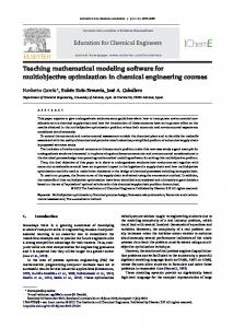
Scip is a framework for constraint integer programming that aims at integrating constraint programming and mixed integer programming into a single solver [1]. It is designed to support the implementation of cp and mip solver components like branching rules, primal heuristics, cutting plane separators, or domain propagators. It allows for a very flexible integration of user-defined non-linear constraints, and it is a fully-fledged branch-cut-and-price framework. Scip comes with a large number of components that suffice to turn the basic framework into a sophisticated mixed integer programming solver. It is able to directly read Zimpl files. Preprocessors transform the problem instance into an equivalent instance that is easier to solve, constraint handlers provide specialized algorithms and data structures to handle specific constraint classes, separators add cutting planes to tighten the lp relaxation, primal heuristics search for feasible solutions, branching rules define the search tree, and node selectors define the way the search tree is processed. To solve the lp relaxations, Scip calls an externally linked lp solver through a basic lp solver interface. In a course on mixed integer programming, Scip can be used to demonstrate and compare the usefulness of certain components, e. g., node selection strategies, branching rules, cut separation algorithms, or primal heuristics. In particular, the search tree can be visualized by using VbcTool [10] which helps to analyze the impact of the employed branching rule and node selection. An example is given in Figure 7, which shows two mip-instances from the miplib [3] solved with the same parameter settings, but producing vastly different branching trees. With the source code at hand, a focus can be set on specific implementation issues, e. g., how one can quickly generate violated clique cuts, or what can be done to ensure numerical stability of Gomory mixed integer cuts. In a more advanced course, students can even implement their own components like a specialized primal heuristic for a given problem class such as the traveling salesman problem. In a course that is primarily focused on modeling, like our workshop Combinatorial Optimization at Work, Scip can be used in conjunction with Zimpl and SoPlex to evaluate ones own mixed integer programming models. Scip as a stand-alone mip solver is easy to use, provides lots of parameters to adjust the solver components, and reports a large number of statistics that show the impact of the different components on the given problem instance.
4
The linear programming solver: SoPlex
SoPlex [14] is an implementation of the revised simplex algorithm for the solution of linear programs. It features primal and dual solving routines and is implemented as a C++ class library that can be used within other programs. SoPlex is under continuous development and the current version as of March 2006 is 1.3.0. An example program to solve standalone linear programs given in mps or lp format files is included. But other than to experiment with parameter settings or for programming exercises 4
there is not much need to use SoPlex as a standalone lp-Solver if Scip is available. Its main use in this context is to act as a solver engine for lp-based mixed integer programming.
5
A puzzling puzzle model
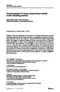
In the following, we use the popular puzzle game named Sudoku [5] to give an impression of how to use Zimpl and Scip to model and solve a problem. The aim of the puzzle is to enter an integer from 1 through 9 in each cell of a 9 × 9 grid made up of 3 × 3 subgrids. At the beginning several cells are already given preset integers. At the end, each row, column and subgrid must contain each of the nine integers exactly once. Figure 1 shows an example. For details see, e. g., http://en.wikipedia.org/wiki/Sudoku. 5
3
4 1 8 5 7 9 2 3 6
4 6 7 1 4 9 8 2
6 2
2 6 9 5 7
3 9 9
8 1 6
4
6 2 3 1 4 8 7 9 5
5 9 7 2 3 6 1 4 8
7 3 1 4 6 2 5 8 9
2 4 9 7 8 5 6 1 3
8 6 5 3 9 1 4 7 2
1 7 6 8 2 3 9 5 4
9 8 4 6 5 7 3 2 1
3 5 2 9 1 4 8 6 7
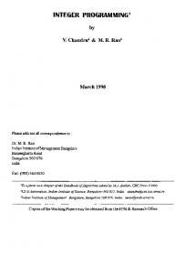
Figure 1: Sudoku puzzle and solution There are several possibilities to model this puzzle. A popular choice is to state the problem as a constraint program using a collection of alldifferent constraints [13]. But how can this be formulated as an integer program? Zimpl can automatically generate ips for certain constructs such as the absolute value of the difference of two variables (vabs). Using 81 integer variables in the range {1, . . . , 9} the alldifferent constraint can be formulated by demanding that the absolute difference of all pairs of relevant variables is greater than or equal to one. This leads to the Zimpl program shown in Figure 2. Note that lines beginning with set define sets, lines with param define parameters, i. e., data, lines starting with var declare variables and lines starting with subto define constraints. Figure 3 shows a Scip session solving the Sudoku instance shown in Figure 1, which is modeled by the Zimpl program of Figure 2. We stripped or slightly relocated parts of the output such that it fits to the size of the paper. As one can see in line 4, parameters can easily be changed with the “set” command. In this case, we impose a time limit of 600 seconds on the solution process. The Zimpl model is read in line 6, generating a mip instance with 3969 variables and 4884 constraints. The large size of the instance arises from auxiliary variables and constraints produced by Zimpl’s automatic modeling of the vabs function. The command “optimize” in line 8 lets Scip solve the instance. Between lines 9 and 29 one can see the solving progress. Presolving is conducted in consecutive rounds, in this case terminating after 66 rounds. The presolving modifications can be seen in lines 13 and 14. After presolving is finished, Scip tries to solve the remaining problem with 1424 variables and 2291 constraints, but the process is interrupted due to the time limit and stops without finding a feasible solution9 . 9
We checked this result with Cplex 9.03, one of the top-of-the-line commercial mip-solvers. After six hours
5
1 2 3 4 5 6
param p set J s e t KK set F param f i x e d [ F ] var x
:= := := := := [J
3; { 1 . . p∗p } ; { 1 . . p } ∗ { 1 . . p }; { r e a d ” f i x e d . d a t ” a s ”” } ; r e a d ” f i x e d . d a t ” a s ”3n” ; ∗ J ] i n t e g e r >= 1 = 1 ; f o r a l l i n J ∗ J ∗ J w i t h j < k do v a b s ( x [ j , i ]− x [ k , i ] ) >= 1 ; f o r a l l i n KK do f o r a l l i n KK∗KK w i t h p∗ i+j < p∗ k+l do v a b s ( x [ ( m−1)∗p+i , ( n −1)∗p+j ] − x [ ( m−1)∗p+k , ( n −1)∗p+l ] ) >= 1 ; f o r a l l i n F do x [ i , j ] == f i x e d [ i , j ] ;
7 8 9 10
s ubto c o l s :
11 12
s ubto s q u a r e s :
13 14 15
s ubto f i x e d :
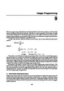
Figure 2: A Zimpl model to solve Sudoku using integer variables The command “display statistics” at line 31 causes the output of a large table with statistical data on the different components and solving steps. One can see that most of the solving time is spent to solve lp relaxations. Two reasons to solve the lp relaxation in a branch-and-bound algorithm are to compute a lower bound for the objective function and to detect infeasibility early. Since Sudoku is a pure feasibility problem it is not possible to compute a bound for the objective function. Also detecting infeasibility seems not to work very effective either, given the huge amount of unprocessed nodes left to compute. Therefore, an idea to improve the performance would be to find better parameter settings for the solver. Figure 4 shows a solving run on the same instance as before, but with different parameter settings. This time we set Scip to perform more like a pure constraint programming solver. In line 4 we select depth-first-search node selection, in line 6 we enable conflict analysis [2] on propagation conflicts, and in line 8 we disable the solving of the lp relaxations. Since we no longer solve the lp relaxations, the branching nodes are processed much faster. The previous run of Figure 3 needed three minutes to process the first 10000 nodes, while this quantity is now processed in 7.4 seconds, as one can see in line 20 of Figure 3 and line 21 of Figure 4. Additionally, mainly due to conflict analysis, a solution is found in 8.2 seconds and 11534 nodes. After displaying the statistics at line 28, the command “display solution” is issued at line 59 to report the optimal solution. The objective value of the solution and all non-zero elements in the solution vector are displayed. In the listing, we only show the output for the first and last model variable. One can see that the Zimpl model generated variable names “x#i#j” with (i, j) being the position in the Sudoku grid. The solution states to use numeral 4 in cell (1, 1) and numeral 7 in cell (9, 9). Choosing the right model is often more important (and more effective) than having the best solver implementation. Especially with real-world problems, having the ability to experiment swiftly with different formulations is essential. Conveying this idea to the students has been a major point in our workshop. Zimpl has proven to be a valuable tool in this regard by letting the students experiment which model works best. For practical work it is important to experience the fact that mathematical equivalent formulations might behave totally different and a million nodes there was still no feasible solution available.
6
1 2
SCIP v e r s i o n 0 . 8 1 f [ p r e c i s i o n : 8 b y t e ] [ mode : o p t i m i z e d ] [ LP s o l v e r : SOPLEX 1 . 3 . 0 ] C o p y r i g h t ( c ) 2002 −2006 Konrad−Zuse−Zentrum f u e r I n f o r m a t i o n s t e c h n i k B e r l i n ( ZIB )
3 4 5 6 7 8 9 10 11 12 13 14 15
SCIP> s e t l i m i t s t i m e 600 p a r a m e t e r < l i m i t s / ti m e> s e t t o 600 SCIP> r e a d s u d o k u i n t . z p l o r i g i n a l pr obl em ha s 3969 v a r i a b l e s (972 bi n , 2997 i n t , 0 c o n t ) and 4884 c o n s t r a i n t s SCIP> o p t i m i z e presolving : ( r ound 1) 24 d e l v a r s , 996 d e l c o n s s , 1014 chg bounds , 0 chg s i d e s , 0 chg c o e f f s ( r ound 65) 2543 d e l v a r s , 2593 d e l c o n s s , 3311 chg bounds , 20 chg s i d e s , 40 chg c o e f f s p r e s o l v i n g (66 r o u n d s ) : 2543 d e l e t e d v a r s , 2593 d e l e t e d c o n s t r a i n t s , 3311 t i g h t e n e d bounds , 20 cha nged s i d e s , 40 cha nged c o e f f i c i e n t s , 23285 i m p l i c a t i o n s p r e s o l v e d pr obl em ha s 1424 v a r i a b l e s (392 bi n , 1032 i n t , 0 c o n t ) and 2291 c o n s t r a i n t s
16 17 18 19 20 21 22 23 24 25
time | 2.9 s | 11.7 s | 176 s | 272 s | 352 s | 426 s | 513 s | 596 s |
node 1 1 10000 20000 30000 40000 50000 60000
| left | LP i t e r | 0 | 1101 | 2 | 13077 | 4013 | 1 1 9 0 0 5 | 7523 | 2 3 1 1 8 3 | 9779 | 3 2 0 1 4 6 | 12171 | 4 0 2 3 5 1 | 14549 | 5 0 4 1 2 5 | 17171 | 6 0 0 2 0 8
| | | | | | | | |
frac 518 764 413 588 498 327 141 −
| r ow s |2123 |3036 |2644 |2644 |2644 |2644 |2644 |2644
| | | | | | | | |
cuts 0 913 913 913 913 913 913 913
| | | | | | | | |
dualbound 0 . 0 0 0 0 0 0 e+00 0 . 0 0 0 0 0 0 e+00 0 . 0 0 0 0 0 0 e+00 0 . 0 0 0 0 0 0 e+00 0 . 0 0 0 0 0 0 e+00 0 . 0 0 0 0 0 0 e+00 0 . 0 0 0 0 0 0 e+00 0 . 0 0 0 0 0 0 e+00
| primalbound | −− | −− | −− | −− | −− | −− | −− | −−
| | | | | | | | |
26 27 28 29
SCIP S t a t u s : s o l v i n g was i n t e r r u p t e d [ t i m e l i m i t r e a c h e d ] S o l v i n g Time ( s e c ) : 6 0 0 . 0 0 S o l v i n g Nodes : 60572
30 31
SCIP> d i s p l a y
statistics
32 33 34 35 36 37 38 39 40 41 42 43 44 45 46 47 48 49 50 51 52 53 54 55 56 57 58 59 60 61 62 63 64
O r i g i n a l Problem : Variables : Constraints : P r e s o l v e d Problem : Variables : Constraints : Presolvers : trivial : dualfix : implics : probing : v a r bound : linear : Constraints : integral : v a r bound : linear : Separators : cut pool : impliedbounds : cmir : clique : Branching Rules : relpscost : LP : d u a l LP : d i v i n g / p r o b i n g LP : strong branching : B&B T r ee : nodes : max d e p t h : backtracks :
number of unprocessed subproblems in search tree
3969 (972 b i n a r y , 2997 i n t e g e r , 0 c o n t i n u o u s ) 4884 i n i t i a l , 4884 maximal 1424 (392 b i n a r y , 1032 i n t e g e r , 0 2291 i n i t i a l , 2291 maximal Time Fixed Aggr ChgBds 0.01 38 0 0 0.00 35 0 0 0.06 0 402 0 1.77 444 114 1726 0.00 0 0 83 0.85 215 1295 1502 Time Number C u t o f f s DomReds 171.60 0 1400 5675 14.68 1723 2619 507022 9.23 568 3770 1221137 Time Calls C u t o f f s DomReds 0.00 6 − − 0.03 7 0 0 0.92 7 0 0 0.00 7 0 0 Time Calls C u t o f f s DomReds 171.40 43452 1400 5675 Time Calls Iters It/ call 248.57 57531 554595 9.64 16.67 3126 50303 16.09 160.34 17903 202879 11.33 60572 107 10778 (17. 8% )
continuous ) D el C ons 0 0 0 0 989 1604 C uts 0 0 0 C uts 3 950 3 2 C uts 0 I t / sec 2231.14 3017.58 1265.30
number of generated implied bound cutting planes
reliable pseudo cost branching was applied time spent in dual simplex to solve relaxations maximal depth of search tree
Figure 3: A Scip session solving a Sudoku instance modeled by Figure 2
7
gap Inf Inf Inf Inf Inf Inf Inf Inf
1 2
SCIP v e r s i o n 0 . 8 1 f [ p r e c i s i o n : 8 b y t e ] [ mode : o p t i m i z e d ] [ LP s o l v e r : SOPLEX 1 . 3 . 0 ] C o p y r i g h t ( c ) 2002 −2006 Konrad−Zuse−Zentrum f u e r I n f o r m a t i o n s t e c h n i k B e r l i n ( ZIB )
3 4 5 6 7 8 9 10 11 12 13 14 15 16 17 18 19 20 21 22
SCIP> s e t n o d e s e l e c t i o n d f s s t d p r i o r i t y 1000000 p a r a m e t e r < n o d e s e l e c t i o n / d f s / s t d p r i o r i t y > s e t t o 1000000 SCIP> s e t c o n f l i c t u s e p r o p TRUE p a r a m e t e r < c o n f l i c t / u s e p r o p > s e t t o TRUE SCIP> s e t l p s o l v e f r e q −1 p a r a m e t e r s e t t o −1 SCIP> r e a d s u d o k u i n t . z p l o r i g i n a l pr obl em ha s 3969 v a r i a b l e s (972 bi n , 2997 i n t , 0 c o n t ) and 4884 c o n s t r a i n t s SCIP> o p t i m i z e presolving : ... t i m e | node | left | v a r s | cons | ccons | conf s | dualbound | primalbound | gap 2.0 s | 1 | 2 |1424 |2291 |2291 | 0 | 0 . 0 0 0 0 0 0 e+00 | −− | Inf 3.2 s | 2000 | 51 | 1 4 2 4 | 2 4 8 4 | 965 | 288 | 0 . 0 0 0 0 0 0 e+00 | −− | Inf 4.4 s | 4000 | 41 | 1 4 2 4 | 2 6 0 7 | 457 | 642 | 0 . 0 0 0 0 0 0 e+00 | −− | Inf 5.4 s | 6000 | 50 | 1 4 2 4 | 2 5 4 9 | 210 | 959 | 0 . 0 0 0 0 0 0 e+00 | −− | Inf 6.4 s | 8000 | 22 | 1 4 2 4 | 2 5 4 7 | 928 | 1 3 1 3 | 0 . 0 0 0 0 0 0 e+00 | −− | Inf 7 . 4 s | 10000 | 11 | 1 4 2 4 | 2 5 6 9 | 942 | 1 6 6 3 | 0 . 0 0 0 0 0 0 e+00 | −− | Inf ∗ 8 . 2 s | 11534 | 0 | 1 4 2 4 | 2 5 9 8 | 157 | 1 9 5 5 | 0 . 0 0 0 0 0 0 e+00 | 0 . 0 0 0 0 0 0 e+00 | 0.00%
23 24 25 26
SCIP S t a t u s : pr obl em S o l v i n g Time ( s e c ) : 8 . 1 7 S o l v i n g Nodes : 11534
i s sol v ed [ optimal
s o l u t i o n found ]
27 28
SCIP> d i s p l a y
statistics
29 30 31 32 33 34 35 36 37 38 39 40 41 42 43 44 45 46 47 48 49 50 51 52 53 54 55 56 57
O r i g i n a l Problem Variables Constraints P r e s o l v e d Problem Variables Constraints Presolvers trivial dualfix implics probing v a r bound linear Constraints v a r bound linear logicor bounddisjunction Conflict Analysis propagation Branching Rules inference B&B T r ee nodes max d e p t h backtracks delayed cu t of f s repropagations
: : : : : : : : : : : : : : : : : : : : : : : : : : : :
3969 (972 b i n a r y , 2997 i n t e g e r , 0 c o n t i n u o u s ) 4884 i n i t i a l , 4884 maximal 1424 (392 b i n a r y , 1032 i n t e g e r , 0 c o n t i n u o u s ) 2291 i n i t i a l , 2615 maximal Time Fixed Aggr ChgBds D el C ons 0.02 38 0 0 0 0.00 35 0 0 0 0.01 0 402 0 0 1.28 444 114 1726 0 0.00 0 0 83 989 0.64 215 1295 1502 1604 Time Number C u t o f f s DomReds C uts 1.57 1723 393 119198 0 1.64 568 1959 285006 0 0.00 0+ 0 8 0 0.17 0+ 61 17496 0 Time Calls Success Confls Lits 0.01 1880 1781 2011 3.0 Time Calls C u t o f f s DomReds C uts 1.50 9560 0 0 0 11534 100 1634 (14. 2% ) 7567 11380 (45088 domain r e d u c t i o n s , 298 c u t o f f s )
number of domain reductions found by linear constraints
constraints added by conflict analysis number of generated conflict constraints used inference branching
58 59
SCIP> d i s p l a y s o l u t i o n
60 61 62 63 64
o bje ct iv e value : x#1#1 ... x#9#9
0 4
( obj :0 )
7
( obj :0 )
Figure 4: Solving the Sudoku model of Figure 2 with CP/SAT techniques
8
in practice. As an alternative we modeled the Sudoku problem using 729 binary variables as shown in Figure 5, instead of 81 integer variables. Figure 6 shows a Scip session for this model on the same data set as before. In this case, presolving managed to fix all variables and to remove all constraints after six rounds. In fact after solving several thousand instances we never encountered a Sudoku instance that could not be solved in preprocessing or in the root node with this model. After presolving has been finished, the remaining trivial empty problem is solved. During the workshop, a new problem area was usually presented each morning in a lecture. In the afternoon, we provided the students with data and a description of the problem setting and let them work out and solve the mathematical modeling on their own. In a course taking place at the University of Bayreuth, we set out a competition for the best performing formulation for the n-Queens problem. And even though the students had only few hours experience with modeling and solving integer programs, they were able to model the problem on their own and beat the formulation of the lecturer.
6
Conclusion
We tested the combination of Scip, Zimpl and SoPlex as the main software environment for the exercises in our two week block course. The problems we posed to the students covered a wide range of applications, including computing the tour of a wielding robot, modeling Sudoku puzzles, solving Steiner tree problems, optimize pizza production, computing OSPF routing weights, modeling telecom network design problems, chip verification, bus routing, driver scheduling, line planning, and repairman tour scheduling problems. The first exercise was to find the minimal number of students that have to change their seats such that everybody without a laptop has a neighbor with a laptop. For the real topology of the lecture hall, this turned out to be much more difficult than initially anticipated. Having the students directly sit down and practically address problems by building a mathematical model and trying to solve it was a great experience. The students developed practical skills and advanced their knowledge both in theory and practice. We received enthusiastic responses within the evaluation after the course. For the course the students had to bring their own laptops. This was very successful for two reasons: first, everybody could work in a familiar environment since the software presented is available for Linux, Windows and Mac-OS alike. And second, after the course the students took home not only their newly acquired knowledge but also their working environment, keeping the ability to actually model and solve problems. All available files from the course including most of the slides and exercises can be found at http://co-at-work.zib.de/download/CD. Further material on using Zimpl and Scip in a course was prepared by J¨org Rambau at the University of Bayreuth and is available at http://www.unibayreuth.de/departments/wirtschaftsmathematik/rambau/Teaching/Uni Bayreuth/WS 2004/Diskrete Optimierung Anwendungen.
Today, companies are forced to rethink their planning methods due to the high innovation pressure. Knowledge in the practical application of mathematical modeling is becoming a key skill in industry, since the solution of mixed integer programs is one of the very few areas which can provide globally optimal answers to discrete (yes or no, choose an option) questions. To teach this knowledge state-of-the-art software as described in this article is required.
9
References [1] Tobias Achterberg. SCIP - a framework to integrate constraint and mixed integer programming. Technical Report 04-19, Zuse Institute Berlin, 2004. [2] Tobias Achterberg. Conflict analysis in mixed integer programming. Technical Report 05-19, Zuse Institute Berlin, 2005. [3] Tobias Achterberg, Thorsten Koch, and Alexander Martin. MIPLIB 2003. Operations Research Letters, 34(4):1–12, 2006. [4] J. Bisschop and A. Meeraus. On the development of a general algebraic modeling system in a strategic planning environment. Mathematical Programming Study, 20:1–29, 1982. [5] David Eppstein. Nonrepetitive paths and cycles in graphs with application to Sudoku. ACM Computing Research Repository, 2005. [6] R. Fourer, D. M. Gay, and B. W. Kernighan. AMPL: A Modelling Language for Mathematical Programming. Brooks/Cole, 2nd edition, 2003. [7] Robert Fourer. Software survey: Linear programming. MS/OR Today, 32, jun 2005. [8] Josef Kallrath, editor. Modeling Languages in Mathematical Optimization. Kluwer, 2004. [9] Thorsten Koch. Rapid Mathematical Programming. PhD thesis, Technische Universit¨at Berlin, 2004. [10] Sebastian Leipert. The tree interface – version 1.0 user manual. Technical Report 96.242, Institut f¨ ur Informatik, Universit¨at zu K¨oln, 1996. [11] J. Linderoth and T. Ralphs. Noncommercial software for mixed-integer linear programming. Optimization Online, 2005. http://www.optimization-online.org/DB FILE/2004/12/1028.pdf . [12] H. D. Mittelmann and P. Spellucci. Decision tree for optimization software, 2006. See http://plato.asu.edu/guide.html. [13] W.J. van Hoeve. The alldifferent constraint: A survey. In 6th Annual Workshop of the ERCIM Working Group on Constraints. Prague, June 2001. [14] R. Wunderling. Paralleler und objektorientierter Simplex. Technical Report TR 96-09, Konrad-Zuse-Zentrum Berlin, 1996.
10
1 2 3 4 5
param p set J s e t KK set F var x
:= 3 ; := { 1 . . p∗ p } ; := { 1 . . p } ∗ { 1 . . p } ; := { r e a d ” f i x e d . d a t ” a s ”” } ; [ J∗J∗J ] b in ary ;
6 7 8 9 10 11
s ubto s ubto s ubto s ubto s ubto
nums : cols : rows : fixed : squares :
12
f o r a l l i n J ∗ J do sum i n f o r a l l i n J ∗ J do sum i n f o r a l l i n J ∗ J do sum i n f o r a l l i n F do f o r a l l i n KK∗ J do sum i n KK : x [ ( m−1)∗p+i
J : x[i J : x[i J : x[i x[i
,j ,j ,j ,j
,k] ,k] ,k] ,k]
== == == ==
1; 1; 1; 1;
, ( n −1)∗p+j , k ] == 1 ;
Figure 5: A Zimpl model to solve Sudoku using binary variables
1 2
SCIP v e r s i o n 0 . 8 1 f [ p r e c i s i o n : 8 b y t e ] [ mode : o p t i m i z e d ] [ LP s o l v e r : SOPLEX 1 . 3 . 0 ] C o p y r i g h t ( c ) 2002 −2006 Konrad−Zuse−Zentrum f u e r I n f o r m a t i o n s t e c h n i k B e r l i n ( ZIB )
3 4 5 6 7 8 9 10 11 12
SCIP> r e a d s u d o k u b i n . z p l o r i g i n a l pr obl em ha s 729 v a r i a b l e s (729 bi n , 0 i n t , 0 c o n t ) and 348 c o n s t r a i n t s SCIP> o p t i m i z e presolving : ( r ound 1) 24 d e l v a r s , 24 d e l c o n s s , 24 chg bounds , 0 i m p l s , 324 c l q s ( r ound 5) 723 d e l v a r s , 324 d e l c o n s s , 614 chg bounds , 236 i m p l s , 0 c l q s p r e s o l v i n g (6 r o u n d s ) : 729 d e l e t e d v a r s , 348 d e l e t e d c o n s t r a i n t s , 619 t i g h t e n e d bounds , 238 i m p l i c a t i o n s p r e s o l v e d pr obl em ha s 0 v a r i a b l e s (0 bi n , 0 i n t , 0 c o n t ) and 0 c o n s t r a i n t s
13 14 15 16
t i m e | node | 0.0 s | 1 | ∗ 0.0 s | 1 |
left
| LP i t e r | f r a c | r ow s | c u t s | dualbound | primalbound | gap 0 | 0 | 0 | 0 | 0 | 0 . 0 0 0 0 0 0 e+00 | −− | Inf 0 | 0 | − | 0 | 0 | 0 . 0 0 0 0 0 0 e+00 | 0 . 0 0 0 0 0 0 e+00 | 0.00%
17 18 19 20
SCIP S t a t u s : pr obl em S o l v i n g Time ( s e c ) : 0 . 0 3 S o l v i n g Nodes : 1
i s sol v ed [ optimal
s o l u t i o n found ]
number of variables that were fixed by linear constraints
21 22
SCIP> d i s p l a y
statistics
23 24 25 26 27 28 29 30 31 32 33 34
O r i g i n a l Problem Variables Constraints P r e s o l v e d Problem Variables Constraints Presolvers trivial linear B&B T r ee nodes
: : : : : : : : : : :
729 (729 b i n a r y , 0 i n t e g e r , 0 c o n t i n u o u s ) 348 i n i t i a l , 348 maximal 0 (0 b i n a r y , 0 i n t e g e r , 0 c o n t i n u o u s ) 0 i n i t i a l , 0 maximal Time F i x e d V a r s A ggr V a r s ChgBounds 0.00 9 0 0 0.01 646 74 619
D el C ons 0 348
1
number of deleted linear constraints
35 36
number of variable aggregations due to linear constraints
SCIP> d i s p l a y s o l u t i o n
37 38 39 40 41
o bje ct iv e value : x#1#1#4 ... x#9#9#7
0 1
( obj :0 )
1
( obj :0 )
42 43
SCIP> q u i t
Figure 6: A Scip session solving a Sudoku instance modeled by Figure 5
11
Figure 7: Comparison of node trees resulting vpm2 and neos3.
12