Software Performance Engineering of Component-based Systems Antonia Bertolino
Raffaela Mirandola
Istituto di Scienza e Tecnologie dell’Informazione “A. Faedo”, CNR Pisa, Italy +39 050 3152914
Dip. Informatica, Sistemi e Produzione Università di Roma TorVergata Roma, Italy +39 06 72597381
[email protected]
[email protected]
ABSTRACT We propose an automated compositional approach for component-based performance engineering, called the CB-SPE. It adapts to a CB framework the concepts and steps of the wellknown SPE technology, and uses for input modeling the standard RT-UML PA profile. The approach is two-layered: it is first applied by the component developer to achieve a parametric evaluation of the components in isolation; then by the system assembler, to predict the performance of the components assembly on the actual platform. We also present the CB-SPE tool architecture and its current status.
1. MOTIVATION AND BACKGROUND Component Based Software Engineering (CBSE) is the emerging paradigm for the development of large complex systems. By maximizing the re-use of separately developed generic components, it promises to yield cheaper and higher quality assembled systems [11]. The basic understood principle (or actually aspiration) is that the individual components are released once and for all with documented properties and that the properties then resulting for the assembled system can be obtained from these in compositional way. While this principle/aspiration has been actively pursued for the system functional properties since the advent of CBSE, it is only recently that equal emphasis is being devoted to the as important non-functional aspects or Quality of Service (QoS), such as reliability, security and performance (e.g., [2,9,12,15]). Our focus is on the evaluation of performance properties (like response time, throughput, etc.): we introduce an automated compositional approach for performance analysis of CB systems by the system assembler. In a companion paper [4], we also present a compositional language to describe a component assembly with adequate information for performance analysis. The approach we propose is called the CB-SPE, which stands for Component-based Software Performance Engineering. CB-SPE is a generalization of the Software Performance Engineering (SPE) (firstly presented in [10]), which is a systematic, quantitative Permission to make digital or hard copies of all or part of this work for personal or classroom use is granted without fee provided that copies are not made or distributed for profit or commercial advantage and that copies bear this notice and the full citation on the first page. To copy otherwise, or republish, to post on servers or to redistribute to lists, requires prior specific permission and/or a fee. WOSP 04, January 14-16, 2004, Redwood City, CA. Copyright 2004 ACM 1-58113-673-0/04/0001 ...$5.00.
approach to construct software systems that meet performance objectives. The original contribution of the CB-SPE approach over the existing SPE is two-fold: on one side, we equipped the CB-SPE of an input modeling notation that is conformant to the standard RT-UML PA sub-profile [13]: this makes the approach more easily usable, also from those designers who are not expert of the specialized (and awkward) performance models, but are familiar with the widespread UML language. On the other side, CB-SPE has been conceived for the analysis of component-based systems, so that the system assembler can derive the performance indices by composing and instantiating the documented component parameters. We have earlier described how the RT-UML PA sub-profile could be adopted to provide an easy-to-use and standard interface to SPE [1]. With regard to the generalization of such methodology to a CB context, while the inspiring ideas have been sketched in [2], in this paper we introduce the steps of the approach by means of an example of application, and the automated tool under development. The paper is organized as follows: after a brief presentation of the methodology in Section 2, we describe the CB-SPE tool structure and functioning in Section 3 and finally in Section 4 we outline an example of application with detailed description of the methodology. Future work is outlined in Section 5.
2. THE CB-SPE APPROACH As its name implies, CB-SPE is proposed as a generalization of the well known SPE approach [10] to CB systems. We generically consider component-based applications, built up from software components glued together by means of some integration mechanism. In this context, the components provide the application-specific functionalities (and are mainly considered as black boxes), and the glue defines the workflow that integrates these functionalities to deliver the services required from the CB application. The CB-SPE approach is applied at two levels, namely the component layer and the application layer. The users of the approach at the two layers are referred below to as the “component developer” (CD) and the “system assembler” (SA).
2.1 The component layer At the component layer, the goal is to obtain components with predicted performance properties (to be used later at the application layer) that are explicitly declared in the component interfaces. Roughly, this implies that the component developer must introduce and validate the performance requirements of the
component considered in isolation, by following the SPE approach. However, in the traditional SPE the component performance properties strongly depend on the execution environment of the component itself, while our goal is to have component performance properties that are platform independent (so that we can eventually use them on the yet unknown platform of the CB application). So in CB-SPE we need to define a component model based on an abstract but quantified specification of the environment, thus obtaining a model not depending on any specific platform (as in [8]). Let us suppose that a given component Ci offers h>=1 services Sj (j=1…h). Each offered service can be carried out either locally (i.e., exploiting only the resources of the component under exam) or externally (i.e., exploiting also the resources of other components). The obtained performance analysis results for each Sj of Ci are exported at the component interfaces, in parametric form, as: PerfCi(Sj[env-par]*) where Perf denotes the performance index we are interested in (e.g., demand of service, response time and communication delay) and [env-par]* a list of environment parameters (e.g., bandwidth, CPU time, memory buffer). In particular, when the service is local, [env-par]* represents the classical platform parameters, such as CPU demand or communication delay, of the node where the component is deployed; while in case of external services, [env-par]* parameters include also demands of resources deployed on nodes that could be different from the one hosting the considered component. An example of the adopted modeling notation based on the standard RT-UML PA profile is given in Figure 1. Component Client
specification
PAresptimeCi(Sj[env-par]*) PAdemandCi(Sj[env-par]*) … PAdelayCi(Sj[env-par]*)
Figure 1:Example of component interface annotations
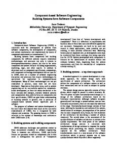
2.2 The application layer Goal of the application layer is to obtain CB applications with the expected performance properties, by the assembly of components whose parametric properties are known. Figure 2 outlines the main steps involved, also highlighting (in italic) who is in charge of each. In summary, the system assembler chooses among the available components those that better fulfil the performance requirements. In fact, at this step, the system assembler knows the characteristics of the environment in which the components will be deployed and thus he/she can instantiate the component performance properties given in parametric form. The various component performance properties can now be combined in a system by following the architecture of the application. If, from the model analysis, the system assembler concludes that the performance requirement are fulfilled, he/she can proceed with the acquisition of the components and their assembly, otherwise he/she has to continue
the search by repeating these steps, or at last declare the unfeasibility of the performance requirements. set of candidate components with performance parametric Input: annotations on the provided interfaces (component developer) Step 1. Step 2. Step 3. Step 4.
Determine the usage profile and the performance goals (system assembler) Component pre-selection/search (system assembler) Modeling and annotation (system assembler) Best/Worst case analysis (automated)
For each couple of candidate SM and MM repeat Step 5. CB-SPE model generation (automated) Step 6. Model evaluation (automated) Step 7. Analysis of results (system assembler) Output: selection of the components and final modeling of the application with performance requirements satisfied, or otherwise declaration of performance requirements unfeasibility
Figure 2: CB-SPE at the application layer
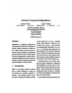
3. APPROACH AUTOMATION The stepwise procedure described above can be partially automated. In principle, steps 4, 5 and 6 (involving the SPE related computations) could be fully automated, while for the other steps, guided support should be provided to the SA to facilitate the RT-UML modeling of the application workflow and of the resource requirements according to the syntax required formats. The tool architecture is illustrated in Fig. 3, where the grey cubes represent the constituent modules of the tool, while the rounded rectangles exemplify the XMI exchanged information. Some parts of this tool are still undergoing development. The Argo-UML [16] tool has been selected as the user interface for UML editing, since it is free and open source. The standard UML diagrams are augmented with performance annotations according to the PA profile. Then Argo automatically processes the input diagrams (with PA annotations) and generates an XML/XMI file that constitutes the input of our Model Generator module. This component (realized in Java) provides, according to the SPE basic principle, two different models (the two different outgoing arcs): a stand-alone performance model, namely an EG, and a contention based performance model, namely a QN model. Let us first describe the round-trip tour for the EG model. Based on [1,3] a global EG is generated from the models of key performance scenarios represented in the SDs (according to their occurrence probability) and its demand vectors are instantiated according to the environment parameters given by the DD. The output of the Model Generator is an XMI document representing the EG. The EG Solver module is a component that applies standard graph analysis techniques [10] to associate an overall “cost” to each path in the obtained EG as a function of the cost of each node that belongs to that path. This stand-alone analysis result gives, for each resource, the total average demand, that, in the optimal case corresponds to the average response time [5]. The Results converter module receives in input both the application performance goals in terms of PA annotations for the different key performance scenarios and the performance results provided by the EG Solver component. A simple comparison can
give insights about the hypothesized component and environment selection as described in the next section. ArgoUML
+ RT-UML PA annotations
tool
UML Model (XMI)
Model Generator component
Results
Performance (XMI)
results
converter
PM solver
Performance Models (XMI)
PM solver
Figure 3: CB-SPE tool architecture Let us now consider the second output of the Model Generator module, that is the QN models. To define a QN model it is necessary to determine: (i) the number of service centers and their characteristics (service discipline, service times) (ii) the network topology and (iii) the jobs in the network with their service demand and routing [5]. For (i) and (ii) the necessary information can be derived from the annotated DDs and SDs. For a first assessment, for example, we associate a QN service center to each DD node. The service center scheduling discipline is derived from the PA annotation and the service can be considered exponential with rate equal to the node throughput (also annotated on the DD). Similarly, the links among the service centers are derived from the ones existing in the DD. The kind of QN (closed, open or mixed) corresponds to the characteristics of the modeled workload (closed, open and mixed, respectively) annotated on the SDs. Concerning the job characteristics (iii), we derive all the essential information from detailed models of key performance scenarios represented in the EGs. The different job classes on the network model the distinct key performance scenarios. The job service demand at network service centers can be computed from the resource demand vectors of the EG. Similarly, the job routing correspond to the application dynamics given by the whole EG.
4. APPLICATION-LAYER ANALYSIS To introduce the stepwise procedure conceived at the application layer, we adopt as a case study a simplified version of a software retrieval application described in [7], composed by 3 or 4 components that interact through different network kinds. There is a user that, through a specialized user interface can select and download new software in an efficient way. A software manager agent obtains the desired catalog through an interaction with a data base and then creates a dedicated catalog agent that helps the user to select the software and performs all the operations required for the desired service. The user can choose to download some software or to browse the catalog of offered services and then select the desired software or can require a catalog refinement. This process can be repeated as many times as necessary. As in [7] we assume that the user accesses the software retrieval service through a wireless mobile device with a low bandwidth. Instead, the interactions between the SW manager, and the catalog agent or the DB take place through a high speed LAN. Now let us describe how the CB-SPE can be applied to this case.
Input Example: Let us suppose that each component is specified following the proposed approach and that the interface presents annotations about its offered/required performance. Step 1: At this step the system assembler should define the different types of application users and the different Use Cases. Let us suppose, for example, that the SA defines the target application A by using four components. A is composed by two different functionalities F1=Browse and F2=Download, that yield a frequency of usage of 0.4 and 0.6, respectively. Following the RT-UML PA profile, the usage profile can be modelled by annotating each Sequence or Activity diagram modeling the Use Case with a PA attribute representing its usage frequency. For the performance goals, the SA, according to the whole application and to its performance requirements, can decide to assign (as in [6]) different importance levels (weights) (i.e., wk) to the various individual performance metric k (e.g., response time, utilization, throughput). wk is a relative importance weight and all weights sum up to 1. In this case, the SA decides that the performance metrics he/she is interested in are the CPU elapsed time with an importance factor w1 equal to 0.7 and the Communication delay with an importance factor w2 equal to 0.3. Step 2: The SA chooses among the components that offer similar services, those that provide the best performance. In fact, he/she can now instantiate the generic PerfCi(Sj[env-par]*) given in the component interfaces, with the characteristics of the adopted (or hypothesized) environment, so obtaining a set of values among which the best ones can be selected. To carry out this choice we can use for instance a metric derived from [6] and reshaped according to this context; we call it perferr. This metric aggregates several performance metrics in a way that is independent of the units of measure of the individual metrics and it increases as the value of an individual metric improves with respect to its bound, while decreases as the value of an individual metric deteriorates with respect to its bound. It is computed as: n
∑wk * fk (∆k )
(1) k =1 where n is the number of metrics being aggregated, wk is the relative importance weight for metric k, ∆k is a relative deviation of the performance metric k defined in a way that the relative deviation is positive when the performance metric satsfies its goal and negative otherwise, and fk (..) is an increasing function of ∆k. For simplicity, in this case, we assume that each component offers a single service S. Thus the annotations in the component interfaces that the SA must instantiate have the form: CPU_DemandCi (S[env-par]*) and Comm_delayCi (S[env-par]*). Then by applying formula (1) with the performance metrics of interest and their relative wk, it is possible to select the combination of components that optimizes the perf-err metric. perf-err =
At the end of this step we assume that the components “UserInterf”, “SW_man”, “Cat-agent” and “DB” are selected. Step 3: The SA should now describe, by one or more sequence diagrams (SD), the application workflow (the glue). Therefore, F1=Browse and F2=Download operations are modeled by means of Argo-UML using User-Interf, SW_man, Cat_agent and DB. For the adopted PA annotations, we have tried to adhere to the RT-UML standard as much as possible; however there are some
aspects, such as message size or use case probability, that are essential for the generation of the performance model, but are not covered by the standard (as also noticed in [1]). For these aspects, that are few ones anyway, we have followed the policy of including “minimal” lightweight extensions. Details of SD interactions for the Browse operation are given in Figure 4. The first note of the SDs describes the kind of workload with its characteristics, using the stereotype PAClosedLoad. We had to define for this stereotype a new attribute, called PAsd, representing the occurrence probability of the modeled scenario. Each step is then annotated with the standard PAstep stereotype, where the attribute PAextop including the message size and the network name models the communication delay involved by the step. Similarly, he/she should construct a Deployment Diagram (DD) modeling the available resources and their characteristics. In this case the nodes of the DD can be associated to classical resources (device, processor, database) and communication means. The
available resources and the possible component/node mappings can be modeled by a DD with standard PA annotations. Step 4: In this step we perform two kinds of static analysis, called Best case and Worst case. A first kind of performance evaluation is called the best-case analysis. This is because the obtained “costs” correspond to the special case of a stand-alone application, i.e., where the application under study is the only one in the execution environment (therefore there is no resource contention), and the application dynamics is taken into account only in terms of component usage frequency. Hence these results provide an optimal bound on the expected performance for each component choice, and can help the system assembler in identifying a subset of components that deserve further investigation in the more realistic setting of application dynamics and of competition with other applications.
Figure 4: SD for Browse operation Let us suppose that the application involves n components Ci and that either the number of services h=1 (∀ Ci) or the application uses only one service at a time for each Ci. Then the performance of the application for a given index is: n
Perf appl =
⊕ i =1
pCi * Perf Ci ( S [env − par ]* )
(2)
where ⊕ denotes a “composition operation” that assumes different meaning according to the performance measure of interest (for example for CPU_demand it becomes a sum), pCi denotes the usage frequency of the component Ci (and all pCi, i=1…n, must sum to one) and is obtained by combining the information derived by the usage profile and the information contained in the SD [3,14]. Similarly, we can derive an optimum bound when the application requires to each component a number h>1 of services.
For functionality F1, the analysis of the SD in Figure 4 for the derivation of pCi leads to: pUI=(2+nb)/(5+2nb), pSM= 2/(5+2nb), pCA=nb/(5+2nb), Pdb=1/(5+2nb). Then the best case analysis for CPU demand and communication delay yields, respectively: CPU_Demand(F1) = p Ui * pCA *
u SSW u SUI + p SM * + x SM * rat SM x MU * rat MU
u SCA u SDB + p DB * x SM * rat SM x LDB * rat LDB
sa + sg + nb * ( sf + se) sb + sc C om m _ delay ( F1) = + * _ * _ v rat wc v rat lan WC LAN
In the previous formulas, uSi, denotes the required service units to the CPUi, xi represents the actual number of service unit/sec that the CPUi processes and rati denotes the percentage of CPU that is
devoted to this task. This information can be derived from the PA annotations on the UML diagrams. The communication delay is given by the ratio between the sum of the exchanged message sizes (sk) and the network speed for this communication (vwc*rat_wc, vlan*rat_lan) also derived from PA annotations. For the sake of generality, the previous formulas are given in parametric form. A similar study can be made for functionality F2. If the required performance for A can be satisfied by the obtained optimal values weigthed by their importance factors, then the process can go on; otherwise the SA can return to step 2.1 With regard to Worst case analysis, we can also compute a pessimistic bound on the application performance by supposing that M (equal or similar) applications compete for the same resources, and that, to obtain a required service, the M-th application must wait, every time, for the completion of the other M-1 applications. The formulae are omitted for space limitations. Step 5: While the results provided in Step 4 provide already some coarse indications, a more realistic performance model should consider the application dynamics, resource contention and communication costs. By the Model generator module we first derive an EG modeling the application example. The second output of the Model generator module is a QN model including the information in the SM modeled by the EG and the components deployment on the given platform according to the modeled DD. Note that we can repeat this (analysis) step on more than one model, so to select the most adequate components. Thanks to the separation between the SM and the MM, we can also investigate different couplings of platforms and software components. Step 6: As already stated the performance measures we are interested in are the CPU-demand and the communication delay. The EG solver module applies first some graph reduction rules. The obtained results from Step 6 give the total CPU demand for the different resources and the communication delay required by the application both for the LAN and for the wireless network. The results obtained from the QN solver are again the CPU demand and the communication delay, but they are more precise, as they include the waiting times for the contended resources. It is possible to observe both local (related to a single resource) and global (related to the whole network) performance indices. Step 7: The results automatically obtained in step 6 are analyzed by the SA and, if different from those expected (or desired), he/she can go back to step 1 (or 2), modify the settled parameters, and repeat the process until the desired results are obtained or after a while the unfeasibility of the performance requirements is declared. To perform this step the SA can apply formula (1) where the performance indexes under exam this time are those relative to the whole application, instead of those of the single component.
5. FUTURE WORK Although this has not been discussed here, the approach can be generalized to allow in turn for incremental compositionality between applications.
1
Note that the optimization of the CPU demand can lead to a greater comm-delay, and vice versa. So, the optimization step can be easy only if there are single performance requirements.
Future work also includes the validation of the proposed methodology by its application to case studies coming from the industrial world. To this purpose, we are now completing the development of the CB-SPE tool, whose architecture has been described. Our long term goal is in fact to include this tool in a general framework for the computer assisted discovery and composition of software components, encompassing both functional and non-functional properties.
6. ACKNOWLEDGMENTS Work partially supported by the MIUR-COFIN project: “SAHARA: Software Architectures for heterogeneous access network infrastructures”, and by Ericsson Lab Italy in the Pisatel initiative: http://www.iei.pi.cnr.it/ERI.
7. REFERENCES [1] Bertolino A., Marchetti, E., Mirandola, R., “Real-Time UML-based Performance Engineering to Aid Manager's Decisions in Multiproject Planning”, in Proc. WOSP 2002. [2] Bertolino A., Mirandola R., “Towards Component-based Software Performance Engineering”, Proc. of CBSE 2003, on line at: http://www.csse.monash.edu.au/~hws/cgibin/CBSE6/Proceedings/pr oceedings.cgi [3] Cortellessa V., Mirandola R. “PRIMA-UML: a Performance Validation Incremental Methodology on Early UML Diagrams”, Science of Computer Programming, 44 (2002), 101-129, July 2002. [4] Grassi V., Mirandola R., “Towards Automatic Compositional Performance Analysis of Component-based Systems”, in Proc. WOSP 2004. [5] Lazowska E.D., et al., “Quantitative System Performance: Computer System Analysis using Queueing Network Models”, on line at : http://www.cs.washington.edu/homes/lazowska/qsp/ [6] Menascé D.A., “Automatic QoS Control” IEEE Internet Computing, Jan.-Feb. 2003. [7] Merseguer J., et al. “Performance evaluation for the design of agentbased systems: A Petri Net approach”. In Proc. of Software Engineering and Petri Nets (SEPN 2000). [8] Selic B., “Performance-Oriented UML Capabilities”. Tutorial talk at WOSP 2002. [9] Sitaraman M., et al., “Performance specification of software components”. Proc. of SSR '01, p. 310. ACM/SIGSOFT, May 2001. [10] Smith, C.U. , Williams L. “Performance Solutions: A practical guide to creating responsive, scalable software”, Addison-Wesley, 2001 [11] Szyperski C., with Gruntz D., and Murer, S., “Component Software: Beyond Object-Oriented Programming”, 2nd Ed., Addison-Wesley, 2002. [12] Wallnau K.C. “Volume III: a technology for predictable assembly from certifiable components” CMU/SEI-2003-TR-009, Apr. 2003. [13] UML Profile for Schedulability, Performance, and Time Specification: on line at: http://cgi.omg.org/docs/ptc/02-03-02.pdf [14] Yacoub S., Cukic B., Ammar H.H “Scenario-based reliability analysis of component-based software”, Proc. ISSRE’99 [15] Yacoub S. “Performance Analysis of Component-Based Application”. Proc. SPLC 2002, p.299-315 [16] www.tigris.org Argo-UML documentation